Multimedia Data Modelling Using Multidimensional Recurrent Neural Networks


1
College of Intelligence Science, National University of Defense Technology, Changsha 410073, China
2
Department of Computer Science, University College London, London WC1E 6BT, UK
3
Department of Computer Science, Sichuan University, Chengdu 610065, China
4
Unmanned Systems Research Center, National Innovation Institute of Defense Technology, Beijing 100071, China
*
Authors to whom correspondence should be addressed.
Symmetry 2018, 10(9), 370; https://doi.org/10.3390/sym10090370
Submission received: 19 August 2018
/
Revised: 23 August 2018
/
Accepted: 27 August 2018
/
Published: 1 September 2018
(This article belongs to the Special Issue Information Technology and Its Applications 2021)
Abstract
:Modelling the multimedia data such as text, images, or videos usually involves the analysis, prediction, or reconstruction of them. The recurrent neural network (RNN) is a powerful machine learning approach to modelling these data in a recursive way. As a variant, the long short-term memory (LSTM) extends the RNN with the ability to remember information for longer. Whilst one can increase the capacity of LSTM by widening or adding layers, additional parameters and runtime are usually required, which could make learning harder. We therefore propose a Tensor LSTM where the hidden states are tensorised as multidimensional arrays (tensors) and updated through a cross-layer convolution. As parameters are spatially shared within the tensor, we can efficiently widen the model without extra parameters by increasing the tensorised size; as deep computations of each time step are absorbed by temporal computations of the time series, we can implicitly deepen the model with little extra runtime by delaying the output. We show by experiments that our model is well-suited for various multimedia data modelling tasks, including text generation, text calculation, image classification, and video prediction.
1. Introduction
Multimedia data such as text, images, and videos are ubiquitous nowadays. Modelling such data usually involves the analysis, prediction, or reconstruction of them. For instance, text modelling relates to many natural language processing tasks such as sentiment analysis [1], part-of-speech tagging [2], machine translation [3], and question answering [4], image modelling relates to many computer vision tasks such as image segmentation [5], depth reconstruction [6], image generation [7], and super-resolution [8], and video modelling also relates to many computer vision tasks such as object tracking [9], video segmentation [10], motion estimation [11], and video prediction [12]. Although they are diverse, these tasks usually can be formulated as a time series prediction problem, e.g., generating a desired output for a given time series , for time , where and are vectors (In this paper, we assume the vectors are in row form). The recurrent neural network (RNN) [13,14] is a popular model that can learn to encapsulate the useful information of the input history into a hidden state vector . By concatenating the input to the previous hidden state , we first get :
The hidden state is then updated by:
where and are parameters namely the weight and bias, respectively; is the activation for , and is the tanh function (element-wise). The RNN finally produces an output for time t:
where and , and is a differentiable transformation that depends on the task.
Nevertheless, the standard RNN is notorious for capturing the long-term dependency caused by the vanishing and exploding gradients [15]. Long Short-Term Memories (LSTMs) [16,17] mitigate this by (i) introducing the memory cell to store information longer, and (ii) utilising the gates for information routing. In a standard LSTM [17], the hidden state is updated as follows:
where and are parameters, are respectively the activations of the input gate , the output gate , the new content , and the forget gate , is the updated memory cell, is the sigmoid function (element-wise), and ⊙ is the element-wise multiplication. Since LSTM is successful in modelling time series, it is natural to further increase its capacity so that it could be profitably applied to a wider range of tasks.
We consider the width and the depth to compose a network’s capacity, where the former measures how much information could be processed in parallel, while the latter measures how many computation steps are required for processing [18]. Whilst using more hidden units in a layer can widen the LSTM, it scales the parameter number quadratically. On the other hand, the Stacked LSTM (sLSTM) deepens the LSTM by using multiple layers [19]; however, the runtime scales linearly with the layer number and the input information is likely to be lost when it vertically passes through the LSTM layers (caused by vanishing/exploding gradients).
The goal of this paper is to make the LSTM wider and deeper and meanwhile prevent its parameter number and runtime from growing. To summarize, we have the following contributions:
- We represent RNN hidden states as multidimensional arrays (tensors) to allow more flexible parameter sharing, thereby being able to efficiently widen the network without extra parameters.
- We use the temporal computations of the RNN to absorb its deep computations in order that we can deepen it without extra runtime. We call this novel RNN as the Tensor RNN (tRNN).
- We propose a memory cell convolution and apply it to the tRNN in order to mitigate gradient vanishing and explosion, obtaining a Tensor LSTM (tLSTM).
- We generalise the tLSTM so that it can process not only non-structured time series (series of vectors) [20], but also structured time series (series of tensors, such as videos).
- We show by experiments that our model is well-suited for various multimedia data modelling tasks, including text generation, text calculation, image classification, and video prediction.
2. Method
2.1. Tensor Representation
From (2), we can see that the parameter number of an RNN scales quadratically with its hidden size. To widen the network while restricting its parameter number, one can use tensor factorisation, where the parameters are represented by multidimensional tensors that could be factorised as low-rank subtensors containing much fewer elements [21,22,23,24,25,26,27,28,29]. As the hidden state vector would be broadcast when interacting with the parameter tensor, the network is widened implicitly. One can also limit the parameter number of an RNN by spatially sharing a small group of parameters within its hidden state, analogous to the convolutional neural network (CNN) [30,31].
Here, we use parameter sharing to reduce the number of parameters in RNNs. In contrast to tensor factorisation, it provides two benefits: (i) scalability—the size of hidden state would not affect the number of parameters; (ii) separability—we can carefully route the information via the receptive field control so that the RNN deep computations can be shifted into its temporal direction (Section 2.2). In addition, the hidden state vectors of RNN are explicitly tensorised, as tensors are more: (i) flexible—we can choose the dimensions for parameter sharing and then just enlarge the sizes of these dimensions so that no more parameters are introduced; (ii) efficient—by using tensors of higher dimensionality, we can widen the network faster when the number of parameters is fixed (Section 2.3).
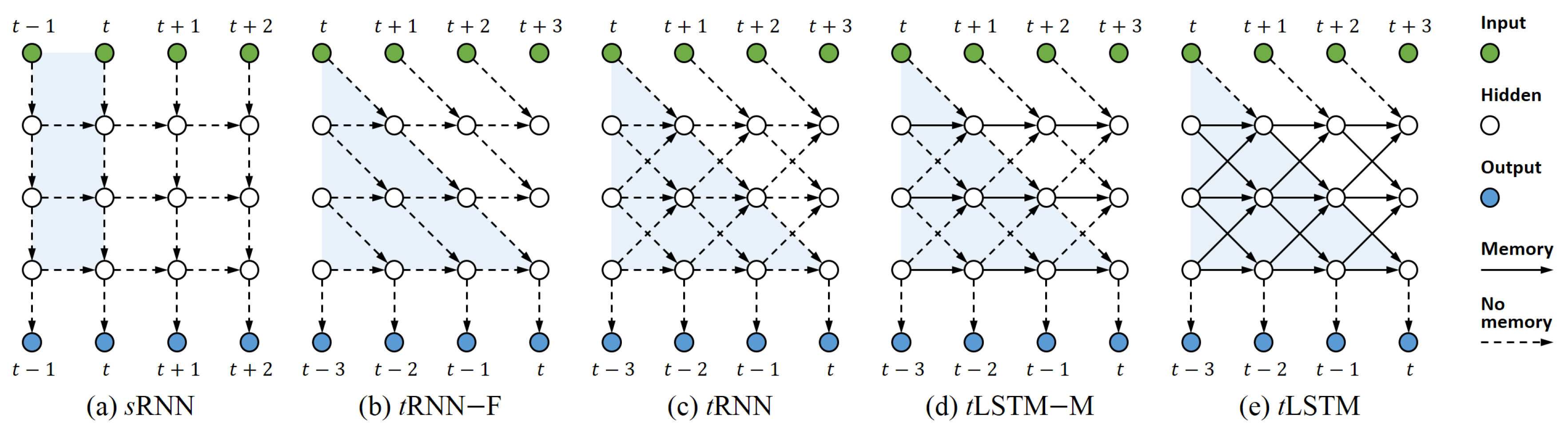
To ease explanation, let’s firstly focus on 2D tensors (matrices). Given a hidden state , we tensorise it as , where P and M are respectively the tensorised size and channel size. In , the 1st dimension is locally-connected for parameter sharing, and the 2nd dimension is fully-connected for global interaction—like in CNN where only the last dimension is fully-connected so that different feature planes (e.g., red/green/blue channels for the input image) can be globally fused. In addition, when comparing with the hidden state in the Stacked RNN (sRNN) (as in Figure 1a), P can be thought as the layer number, and M can be thought as each layer’s size. To explain our model, we start with 2D tensors, and then demonstrate how to use higher dimensional tensors to enhance the model, and finally show how to extend the model to deal with structured input time series.
2.2. Deep Computation through Time
As RNN is already deep when unfolded in time, we can associate the input with a future (delayed) output to also make the input-to-output computation deep. To achieve this, we should guarantee that the output is separable, i.e., it is independent of the future input . Therefore, we first stack ’s projection on top of ; then move the input content downwards through the temporal computation, and finally produce from the bottom of a future hidden state , where denotes the delayed time steps and L denotes the depth. Figure 1b shows an example with , which can be thought as a skewed sRNN that is mentioned in [7,32]. However, in our implementation, the network structure does not need to be changed, and various interactions are also allowed if the output satisfies the separability. For instance, we can use wider local connections or introduce feedback connections (as in Figure 1c) to improve the model (similar to [33]). In addition, we update by convolving it with a learnable kernel so that the parameters can be shared. In doing this, we have increased the input–output mapping complexity (via output delay) and limited the growth of the parameter number (via parameter sharing by convolution).
To define the above described tRNN, we denote the concatenated hidden state as , and the location at a tensor as . At location p of , the channel vector satisfies:
where and . The hidden state is then updated through a convolution:
where and are the kernel’s weight and bias, respectively, with K denoting the kernel size, the input channel, and the output channel, denotes the activation of , and ⊛ denotes the convolution operation (detailed in Appendix A.1). As kernels convolve across different layers of the hidden state, we call the convolution as a cross-layer convolution, which allows the interaction among layers (from both top-down and bottom-up). Finally, the channel vector , located at the bottom of , is used to generate :
where and . To ensure ’s receptive field only covers historical inputs (as in Figure 1c), a constraint among L, P, and K needs to be satisfied:
where % is the modulus operator and ⌈·⌉ denotes the ceil operation. Please see in Appendix B for the derivation of (13).
We call the RNN described in (9)–(12) as a Tensor RNN (tRNN), where one can increase the tensorised size P to widen the model, and meanwhile keep the number of parameters fixed (by using convolution). Moreover, different from the sRNN with a runtime complexity of , the runtime complexity of a tRNN is broken down to , indicating that the runtime would not be significantly affected by T or L.
2.3. Using LSTMs
To capture the long-term dependency across different time steps, the tRNN can be straightforwardly extended with LSTM by modifying (10) and (11) as:
where is the kernel with kernel size K, input channel , and output channel , are respectively the activations of the input gate , the output gate , the new content , and the forget gate , and is the updated memory cell. However, as (16) only gates the previous memory cell along the temporal direction (as in Figure 1d), when the tensorised size P grows large, the long-term dependency from the input–output direction is likely to be lost.
2.3.1. Memory Cell Convolution
Here, we propose a novel memory cell convolution (memConv) for capturing the long-term dependency from multiple directions, where, like the hidden state, the memory cell could also have a wider receptive field (as in Figure 1e). In addition, the kernel for memConv is generated on the fly and therefore varies with time and location, flexibly controlling the long-term dependency from different directions. Concretely, we define the tensor update for tLSTM as follows:
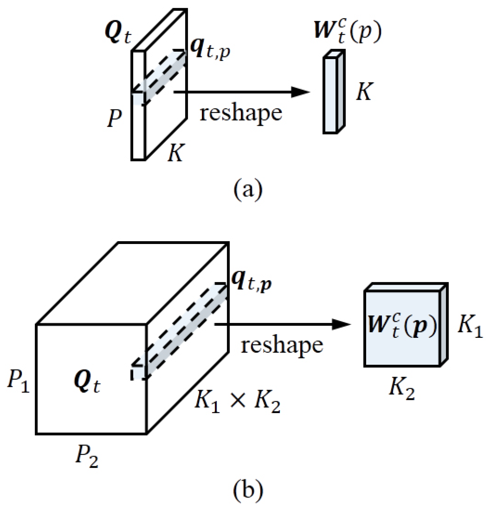
where, unlike (14)–(17), the kernel contains additional output channels ( computes the cumulative product of the input variable elements) for generating the activation of the dynamic kernel bank , denotes the vectorised dynamic kernel selected from ’s entry p, and is the dynamic kernel reshaped from (illustrated in Figure 2a), with a size K and a single input/output channel. Equation (21) defines the memConv (detailed in Appendix A.2), where we use , the value of which varies with p, to convolve every channel of , producing a convolved memory cell . Analogous to [34], in (19), a softmax function is employed to normalise along its channel dimension, which can stabilise the memory cell values and thereby mitigate the vanishing and exploding gradients (please check Appendix C for more discussion).
There are many works [22,23,27,35,36,37] using the concept of dynamically producing the model weights, where [36] also dynamically generates location-dependent convolution kernels for improving the CNN. Unlike these works, we aim to broaden the receptive fields for tLSTM memory cells. Whilst being flexible, fewer parameters are needed for generating the memConv kernel as it can be shared by different channels of the memory cell.
2.3.2. Channel Normalisation
We adapt the recently proposed layer normalisation (LN) [38] to speed-up the training of tLSTM. In [38], LN has been observed unsuitable for the CNN where different statistics are possessed by different channel vectors. Similarly, we have found that LN also performs not well for the tLSTM, in which low-level information is possessed by channel vectors close to the input and vice versa. Therefore, we propose a channel normalisation (CN), which normalises each channel vector independently. The CN operator is defined as:
where , and are parameters namely the gain and bias, respectively, is the input tensor, and is the normalised tensor. Let be the -th channel of , it is normalised element-wisely:
where are respectively the mean and the standard deviation which are computed along ’s channel dimension, and denotes the -th channel in . As the parameter number introduced by CN/LN is quite small in terms of the model parameters, it could be reasonably neglected.
2.3.3. Leveraging Higher-Dimensional Tensors
In (13), we can see that given the kernel size K, the tensorised size P scales linearly w.r.t. the depth L. To widen the tLSTM more efficiently, we resort to using higher-dimensional tensors, where the tensor volume can be expanded more rapidly. Based on the tLSTM defined in previous sections, we can generalise the tensors from 2D to -dimensional where , resulting in with the tensorised size . As the hidden states are more than 2D, we instead concatenate ’s projection to the corner of , thereby extending (9) as:
where the channel vector is the entry of the concatenated hidden state . Accordingly, the output is generated at the opposite corner of , thus we modify (12) as:
To update the hidden state, we also tensorise the convolution kernel and so that they have a kernel size of , where is still reshaped from the vector (see Figure 2b). In order to make every dimension of P and K meet the constraint (13) with a same L, we set and for . For CN, it is still applied to normalise the channel dimension of tensors.
2.4. Handling Structured Inputs
Until now, we have limited our discussion to the case where the input at each time step is a vector, which is non-structured. However, as structured data (e.g., image time series) also emerges in many multimedia modelling tasks (e.g., video segmentation, motion estimation, and video prediction), it is essential to generalise the model to handle structured inputs.
We use to denote the structured input at time step t, where is the structure dimensionality and the structure size, e.g., when is a 2D image, then is the image size (height and width) and U is the image depth (channel). Correspondingly, we have a hidden state . In contrast to (26), we define the sub-tensor locating at entry of as:
where the convolution kernel is used for linear projection and is of size , with U input channels and M output channels.
To update the hidden state tensor, the size of convolution kernels and becomes , where the first D dimensions, , are related to the tensorised size , and the succeeding E dimensions, , are related to the structure size . This also means that are free of the constraint (13).
Finally, we generate the output from the sub-tensor . Note that for many tasks such as video prediction, the output usually has the same structure (i.e., a same ) as the input. In this case, the output can be generated by:
where is the structured output and is the convolution kernel of size , with M input channels and V output channels. In addition, it is straightforward to generate a non-structured output from , e.g., by using a CNN or a fully-connected network.
3. Related Work
3.1. Convolutional LSTMs
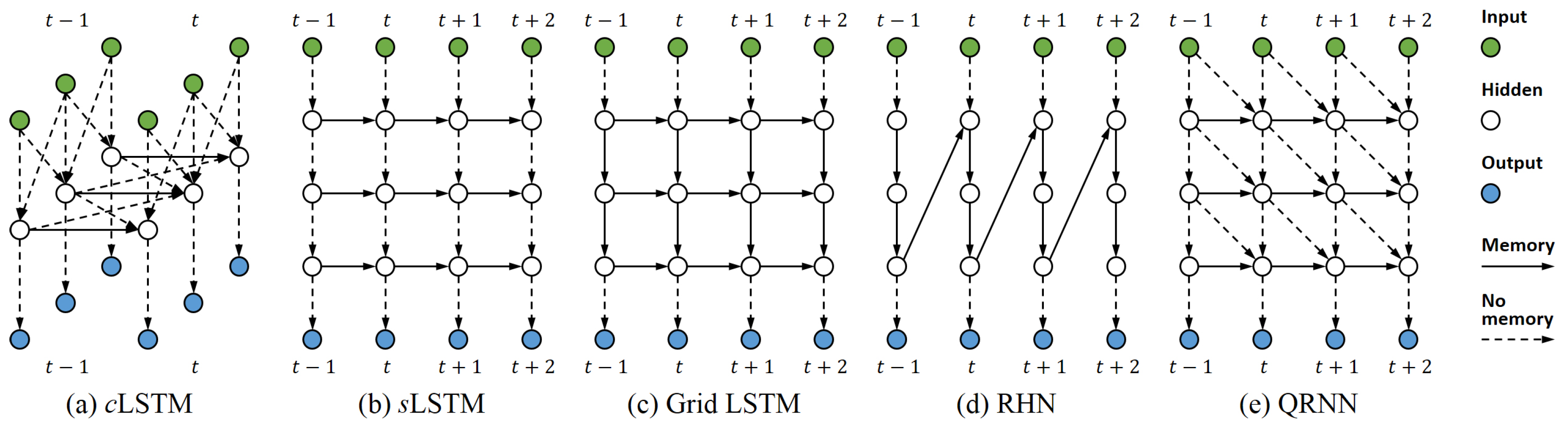
The Convolutional LSTM (cLSTM) parallelises the computation of LSTM where at each time step the input is structured (as in Figure 3a), such as an array vector [7], a matrix of vectors [39,40,41,42], and a tensor of vectors [43,44]. Different from the cLSTM, tLSTM focuses on increasing the capacity of LSTM where each input can also be non-structured (a single vector), and has the following advantages: (i) the convolution in tLSTM is performed across different hidden layers, the structure of which can be different from the input structure, integrating information top-down and bottom-up, whereas the convolution in cLSTM is only performed within each hidden layer, the structure of which depends on the input structure, thereby falling back to the standard LSTM when each input is a single vector; (ii) by increasing the tensorised size, one can efficiently widen the tLSTM without introducing more parameters, whereas to widen the cLSTM, either increasing the kernel size or kernel channel can significantly increase the parameter number; (iii) by delaying the output, one can deepen the tLSTM with little additional runtime, whereas to deepen the cLSTM, increasing the number of hidden layers can significantly increase the runtime; (iv) with the memConv, tLSTM can capture the long-term dependency of multiple directions, whereas, cLSTM only gates the memory cell along one direction, thereby struggling to capture the long-term dependency of multiple directions.
3.2. Deep LSTMs
The Deep LSTM (dLSTM) improves the sLSTM by further deepening it (as shown in Figure 3b–d). In order to limit the number of parameters as well as make training easy, in [46,47,49,50], another RNN/LSTM is applied to the depth direction of dLSTMs. However, the runtime is still multiplied by the depth. Though deep computations are accelerated in [32,51], they mainly focus on simple architectures, e.g., sLSTMs. Unlike dLSTMs, in tLSTM, deep computations are performed with little extra runtime, and feedback is enabled by cross-layer convolutions. Furthermore, by utilising higher dimensional tensors, one can increase tLSTM’s capacity with higher efficiency, while the whole stacked hidden layers in a dLSTM only compose a 2D tensor, whose dimensionality is fixed.
3.3. Other Parallelisation Methods
When full input and target sequences are available for training, temporal computations of the time series are parallelised (for instance, by using temporal convolutions like in Figure 3e) in [48,52,53,54,55,56]. Nevertheless, for online inference, since inputs are presented sequentially, these methods can no longer parallelise temporal computations, which will also be blocked by deep computations of each time step, rendering themselves not well-suited for the real-time application which requires a high sampling/output frequencies. On the contrary, as tLSTM performs deep computations through temporal computations, it can accelerate both training and online inference for many tasks. This is human-like: when converting the input signal into action, we simultaneously process newly arrived signals in a nonblocking manner. One should also notice that for some tasks (such as autoregressive sequence generation) which take the previous output as the current input , tLSTM is unable to parallelise the deep computation for online inference, since additional time steps are required to generate for each .
4. Experiments
To evaluate our tLSTM, we experiment on seven challenging multimedia data modelling tasks, and are interested in the following configurations:
- sLSTM: We implement the sLSTM [45] and share the parameters for different layers. This configuration is served as our baseline.
- 1-tLSTM–F: 1-tLSTM with no feedback connection (–F).
To make different configurations comparable, for sLSTM, we use L and M to represent the layer number and the size of each layer, respectively. Let K be the value of the first D dimensions of the kernel size , we set for 1-tLSTM–F and for other tLSTM configurations, so that according to (13), we have .
To check if tLSTM’s performance can be improved without using additional parameters, for each configuration, we use the same amount of parameters and meanwhile increase the tensorised size. We also inspect how the depth can affect the runtime, which is quantified as the averaged milliseconds cost by a single sample’s forward and backward passes over a single RNN time step. Then, we evaluate tLSTM’s ability by comparing it against the state-of-the-art methods. Finally, we analyze the inner working of tLSTM by visualising its memory cells.
The training objective is to minimise the training loss w.r.t. the parameter (vectorised), i.e.,
where N is the number of training sequences, is the length of the n-th training sequence, and is the loss between the prediction and the target. We define as the Mean Squared Error (MSE) for regression problems (our video prediction tasks), and as the cross entropy for classification problems (our other tasks). In all tasks, the training objective is minimised by Adam [57] with a learning rate of 0.001. Forget gate biases are set to 4 for image classification tasks and 1 [58] for others. All models are implemented by Torch7 [59] and accelerated by cuDNN on Tesla K80 GPUs (NVIDIA, Santa Clara, CA, USA).
We only apply CN to the output of the tLSTM hidden state as we have tried different combinations and found this is the most robust way that can always improve the performance for all tasks. With CN, the output of hidden state becomes:
4.1. Text Generation
The dataset of Hutter Prize Wikipedia [60] is a text file comprising 100 million characters with a vocabulary size of 205, including alphabets, special symbols, and XML markups. This dataset is modelled at character-level, and the goal is generating the next character given all previous ones, e.g.,:
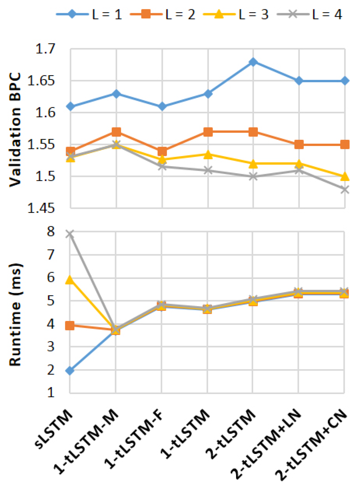
We evaluate all configurations for the depth and use 10 M parameters, so that the channel size M for sLSTM and 1-tLSTM–F is 1120, for other 1-tLSTMs is 901, and for 2-tLSTMs is 522. Bits-per-character (BPC) are used for performance measuring. As in [33], we split the dataset into 90 M/5 M/5 M for training/validation/test. In each iteration, the model is fed with a mini-batch of 100 subsequences of length 50. During the forward pass, the hidden values at the last time step are preserved to initialise the next iteration. We terminate training after 50 epochs.
Figure 4 shows the results. With a larger M, sLSTM and 1-tLSTM–F perform better than other models when . When L increases, sLSTM and 1-tLSTM–M boost their performances but get stuck when , whereas, with the memConv, the performances of tLSTMs improve, finally surpassing sLSTM and 1-tLSTM–M. With , the performance of 1-tLSTM–F is exceeded by that of 1-tLSTM, which is exceeded by that of 2-tLSTM in turn. Whilst LN benefits 2-tLSTM only when , CN consistently benefits 2-tLSTM with different L.
Note that, in each tLSTM configuration, the runtime is nearly constant and largely unaffected by L, while in sLSTM, the runtime is almost proportional to L.
4.2. Text Calculation
- (i)
- Addition: The goal of this task is adding two integers of 15-digit. The model firstly reads both integers, after which it predicts their sum, both in a sequential manner (i.e., one digit per time step). Following [46], we use the symbol ‘-’ to delimit integers and pad the input and target sequences, e.g.,
- (ii)
- Copy: The copy task is to reproduce 20 random symbols presented as a sequence, where 65 different symbols are used. As in the addition task, the symbol ‘-’ is also used as a delimiter, e.g.,
For the addition and copy tasks, we set M to 400 and 100, respectively, and evaluate each configuration for . The prediction accuracy of symbols are used to measure the performance. Like in [46], for both tasks we randomly generate 5 M training samples and 100 test samples, and set the mini-batch size to 15. Training proceeds for at most one epoch (To simulate the online learning process, we use all training samples only once) and will be terminated if test accuracy is achieved.
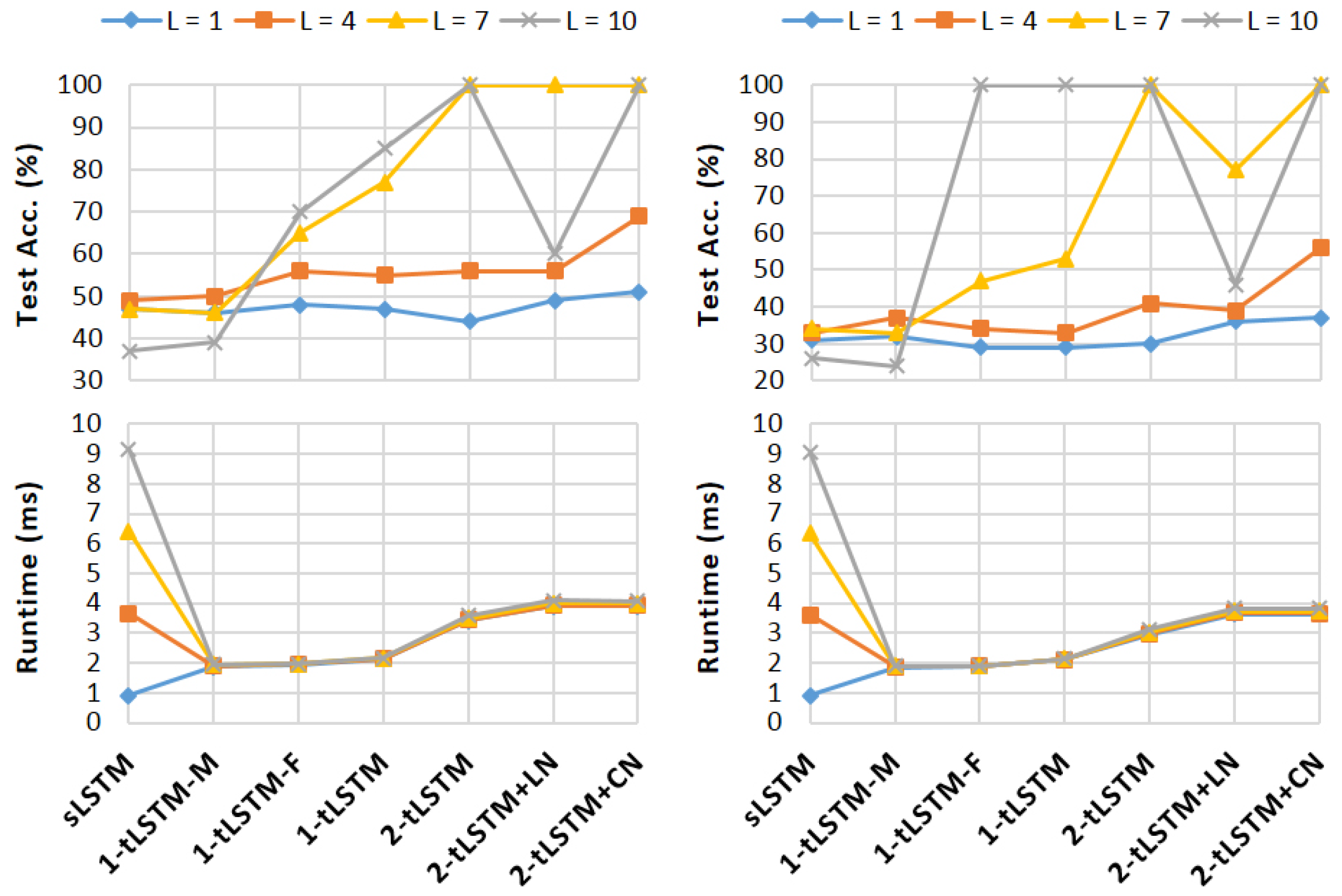
Results are shown in Figure 5. In both tasks, the performances of sLSTM and 1-tLSTM–M degrades with larger L. On the contrary, with L increasing, the performance of 1-tLSTM–F continues improving, and can be further boosted by using feedback, tensors of higher dimensionality, and CN, whilst LN improves the performance only when . Note that correct solutions can be found (when achieving test accuracies) in both tasks because of their repetitive nature. From the experiments, we find that in the task of addition, 2-tLSTM+CN of performs the best and solves the task using only 298 K training examples, whilst in the task of copy, 2-tLSTM+CN of outperforms other configurations and copies perfectly using only 54 K training examples. Moreover, different from sLSTM, all tLSTMs’ runtime can be largely independent of L.
On both tasks, the best performing configurations are further compared to the state-of-the-art methods. Table 2 reports the results. Our model solves the tasks of both addition and copy significantly faster (with fewer training examples) than others, being the new state-of-the-art.
4.3. Image Classification
The dataset of MNIST [31] comprising 70,000 handwritten digit images sized , which is divided into 50,000/10,000/10,000 for training/validation/test. For this dataset, there are two tasks:
- (i)
- Sequential MNIST: In this task, the model first sequentially reads the pixels in a scanline order, and then outputs the class of the digit contained in the image [62]. It is a time series task of 784 time steps, where we generate the output from the last time step, thereby requiring to capture very long term temporal dependencies.
- (ii)
- Sequential Permuted MNIST: To make the problem even harder, we generate a permuted MNIST (pMNIST) [63] by permuting the original image pixels with a fixed random order so that the long-term dependency can also exist in neighbouring pixels.
In both tasks, we evaluate all configurations with and . We employ the classification accuracy to measure the model performance. We set the mini-batch size to 50, and use early stopping for training. The training loss is calculated at the last time step.
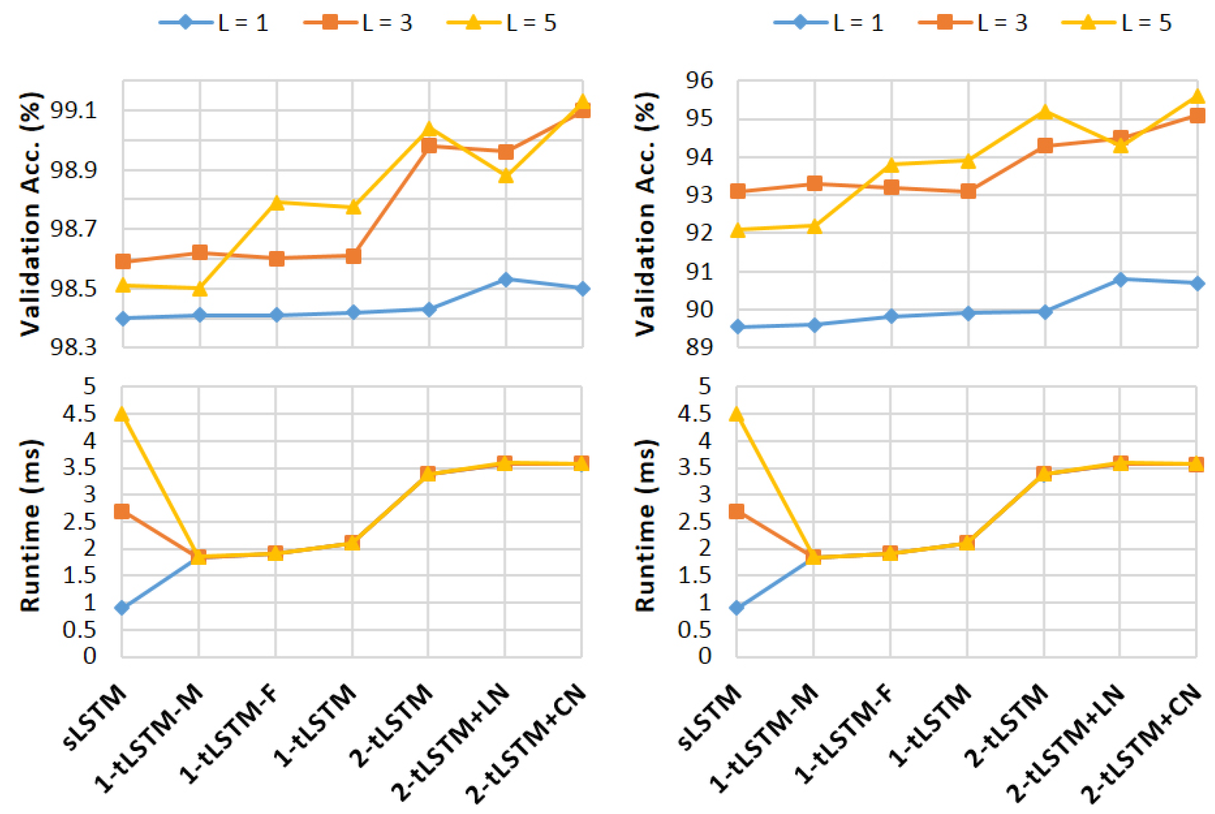
Figure 6 shows the results. Increasing the depth no longer benefits sLSTM and 1-tLSTM–M when , while the performance of 1-tLSTM can be boosted by a larger depth and tensorisation. However, the performance of 1-tLSTM seems not to be affected by removing the feedback connections. In addition, CN always improves 2-tLSTM and outperforms LN when . With validation accuracies of 99.1% on MNIST and 95.6% on pMNIST, 2-tLSTM+CN with outperforms all other configurations in both tasks. In tLSTMs, the runtime is little affected by L, and when , all tLSTMs runs faster than sLSTM.
As presented in Table 3, the best performing configurations are compared against the state-of-the-art methods. On sequential MNIST, 2-tLSTM+CN with achieves 99.2% test accuracy, which is the same as the state-of-the-art one produced by the Dilated GRU [56]. On sequential pMNIST, 2-tLSTM+CN with achieves 95.7% test accuracy, approaching the state-of-the-art one of 96.7% which is obtained from the Dilated CNN [54] in [56].
4.4. Video Prediction
The task of video prediction aims at predicting the future frames of a video given the historical frames. It has a variety of applications such as environment simulation, dataset augmentation, and many computer vision tasks. The main challenge is that the model must capture both the spatial and the temporal relationships among data well. We apply our model to two datasets:
- (i)
- KTH [67]: The dataset consists of 600 real videos with 25 subjects performing six actions (walking, running, jogging, hand-clapping, hand-waving, and boxing). It has been split into a training set (subjects 1–16) and a test set (subjects 17–25), resulting in 383 and 216 sequences, respectively. We resize all frames to .
- (ii)
- UCF101 [68]: The dataset consists of 13,320 real videos of resolution with 101 human actions that could be split into five types (sports, playing musical instruments, human-human interaction, body-motion only, and human-object interaction). It is currently the most challenging dataset of actions. Following [69], we train our models on Sports-1M [70] dataset and test them on UCF-101.
On both tasks, we evaluate all configurations with . To process the structured inputs (i.e., video frames), we modify the original sLSTM [45] by replacing each LSTM layer with a Convolutional LSTM [39], where the convolution kernel size is set to . We also set the last two dimensions (relevant to image structure) of the convolution kernel size to 5 for tLSTMs. M is set to 100 for KTH and 200 for UCF101. The model performance is measured by three common metrics including MSE, Peak Signal-to-Noise Ratio (PSNR), and Structural Similarity Index Measure (SSIM) [71], where SSIM ranges in (larger is better). We set the mini-batch size to 16 and employ early stopping for training. All models are trained by observing 10 frames and predicting the next 10 frames.
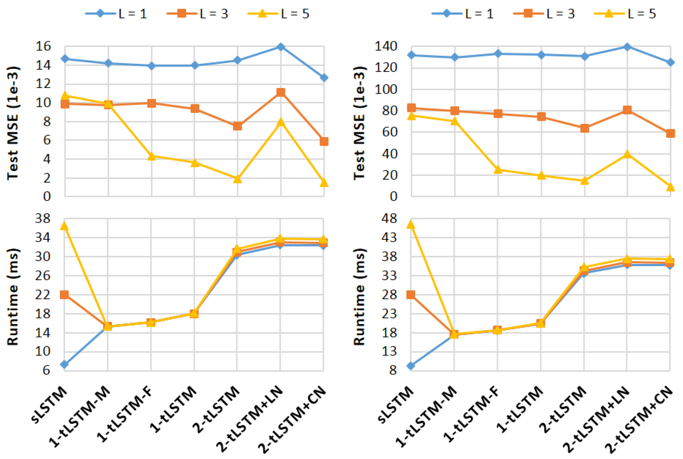
Figure 7 shows the quantitative results. When L increases, sLSTM and 1-tLSTM–M improve their performances but get stuck at , while with the memConv, the performances of tLSTMs improve and finally exceed both sLSTM and 1-tLSTM–M. The effects of feedback and tensorisation become significant when L is large. Similar to the finding in [38] that LN is not suitable for normalising the convolution layer for images, the performance of 2-tLSTM+LN is even worse than 2-tLSTM. However, CN improves 2-tLSTM with different L. Unlike sLSTM where the runtime increases linearly w.r.t. L, tLSTM can keep its runtime largely unchanged when increasing L.
The best performing configuration is compared with the state-of-the-art methods (their source codes are publicly available) on both datasets (see Table 4). 2-tLSTM+CN with outperforms all existing models on KTH w.r.t. all metrics, and on UCF101 w.r.t. MSE and SSIM. Sampled qualitative results produced by 2-tLSTM+CN are shown in Figure 8.
4.5. Analysis
It can been seen from the experiments that one can boost the performance of tLSTMs by enlarging the tensorised size or increasing the model depth, whereas almost no extra parameters and runtime are required. The memConv is indispensable to maintain the performance improvement when the network gets wider and deeper. In addition, for tasks with sequential output, feedback connections are useful. In addition, tensorisation or CN can further strengthen the tLSTM.
To inspect the inner working of our tLSTM, the value of memory cells are visualised to show the information routing. On each task, we run the best performing tLSTM with a random sample (here we do not consider video prediction tasks where memory cells of the 2-tLSTM are 5D tensors, which are hard to visualise). At each time step, we record the memory cell’s channel mean (computed by averaging along the channel dimension, for the 2-tLSTM, it has a size of ), and visualise its diagonal values from location (close to the input) to (close to the output).
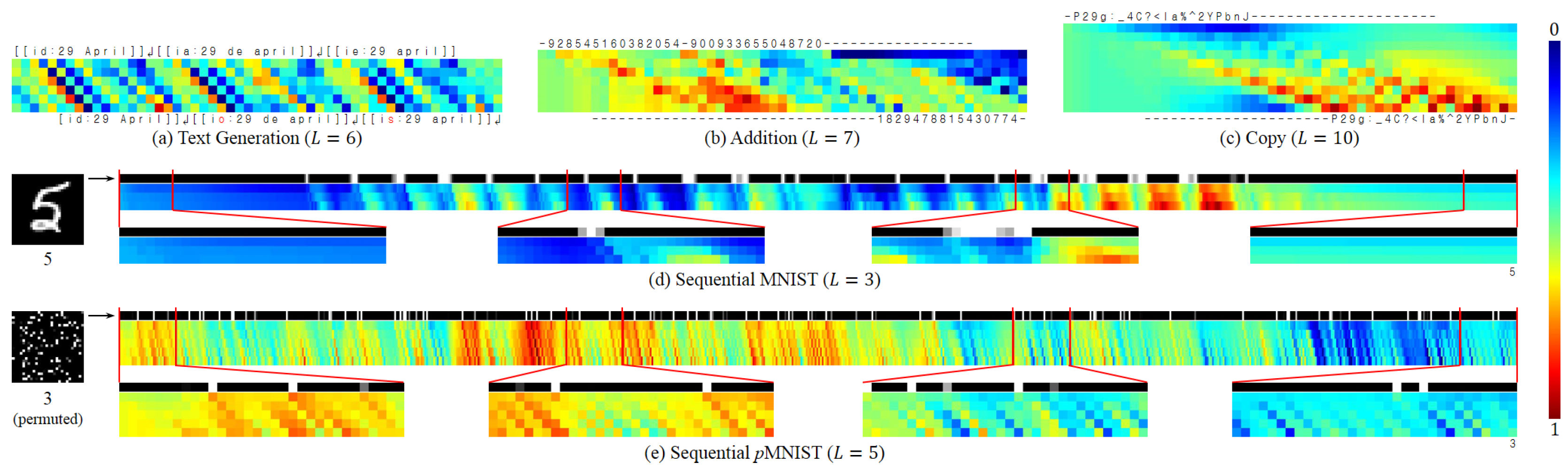
As shown in Figure 9, the visualisation result reveals different behaviors of tLSTM when handling different tasks:
- Text Generation: If the next character is largely determined by the current input, the input content can be preserved with less modification when it arrives at the output location, and vice versa.
- Addition: Two integers are gradually compressed into the memory and then interact with each other, generating their summation.
- Copy: The model acts as a shift register, continuing to move the input symbols to their output locations.
- Seq. MNIST: The model seems more sensitive to pixel value changes (which represent contours, or the digit topology); it gradually accumulates evidence to generate the final output.
- Seq. pMNIST: The model seems more sensitive to high value pixels (which come from the digit); our conjecture is that the permutation has destroyed the digit topology, and thereby made each high value pixel potentially important.
In these tasks, there are also some common phenomena:
- At each time step, different locations of the tensor possess markedly different values, which implies that a tensor of a larger size could encode more content, requiring less effort for compressing.
- The value becomes more and more distinct from the input to output and is shifted along the time axis, which reveals that the model indeed simultaneously performs the deep and temporal computations, with the memory cell carrying the long-term dependency.
5. Conclusions
In this paper, we have aimed to deal with multimedia modelling tasks. We have introduced the tLSTM, where tensors are employed to share parameters and temporal computations are utilised to perform deep computations. The main advantage of our tLSTM over other popular methods is that its capacity can be increased with almost no extra parameters and runtime. Another important advantage of the tLSTM is that it can handle a variety of challenging multimedia modelling tasks well as shown in our experiments.
For future work, we would like to: (i) investigate more about the effect of higher-dimensional tensors, e.g., try 3- and 4-tLSTMs, (ii) try increasing the transition depth for tLSTM hidden states (similar to [47]); and (iii) apply tLSTMs to more multimedia modelling tasks such as machine translation, image generation, and video segmentation.
Author Contributions
Methodology, Z.H., S.G., L.X., D.L., and H.H.; Software, Z.H. and S.G.; Validation, Z.H. and L.X.; Investigation, Z.H., S.G., and D.L.; Writing—Original Draft Preparation, Z.H.; Writing—Review & Editing, Z.H., S.G., D.L., and H.H.; Visualization, Z.H., S.G., and L.X.; Supervision, D.L. and H.H.; Project Administration, Z.H., D.L., and H.H.
Funding
This work is supported by the Natural Science Foundations of China under Grants 91220301 and 61806134.
Conflicts of Interest
The authors declare no conflict of interest.
Appendix A. Mathematical Definition for Cross-Layer Convolutions
Appendix A.1. Hidden State Convolution
The hidden state convolution in (10) is defined as:
where and we apply zero padding to maintain the tensorised size.
Appendix A.2. Memory Cell Convolution
The memory cell convolution in (21) is defined as:
To prevent the stored information from being flushed away, is padded with the replication of its boundary values instead of zeros or input projections.
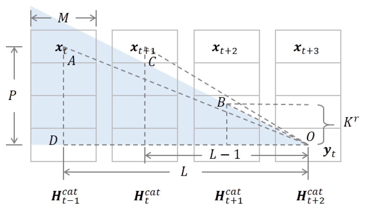
Appendix B. Derivation for the Constraint of L, P, and K
Here we derive the constraint of L, P, and K that is defined in (13). The kernel center location is sealed in case the kernel size K is not odd. Then, the kernel radius can be calculated by:
As shown in Figure A1, to guarantee that the receptive field of covers while not covering , the following constraint should be satisfied:
which means:
Figure A1.
Illustration of calculating the constraint of L, P, and K. Each column is a concatenated hidden state tensor with tensorised size and channel size M. The volume of the output receptive field (blue region) is determined by the kernel radius . The output for current time step t is delayed by time steps.

Appendix C. MemConv Mitigates the Gradient Vanishing/Explosion
In [34], it has been proved that the lambda gate, which is very similar to our memConv kernel, can mitigate the gradient vanishing/explosion (please refer to Theorems 17 and 18 in [34]). The differences between our approach and their lambda gate are: (i) we normalise the kernel values though a softmax function, while they normalise the gate values by dividing them with their sum, and (ii) we share the kernel for all channels, while they do not. However, as neither modifications affects the conditions of validity for Theorems 17 and18 in [34], our memConv can also mitigate the gradient vanishing/explosion.
References
- Socher, R.; Perelygin, A.; Wu, J.; Chuang, J.; Manning, C.D.; Ng, A.; Potts, C. Recursive deep models for semantic compositionality over a sentiment treebank. In Proceedings of the 2013 Conference on Empirical Methods in Natural Language Processing, Seattle, WA, USA, 18–21 October 2013. [Google Scholar]
- Santos, C.D.; Zadrozny, B. Learning character-level representations for part-of-speech tagging. In Proceedings of the 31st International Conference on International Conference on Machine Learning, Beijing, China, 21–26 June 2014. [Google Scholar]
- Bahdanau, D.; Cho, K.; Bengio, Y. Neural machine translation by jointly learning to align and translate. In Proceedings of the International Conference on Learning Representations 2015, San Diego, CA, USA, 7–9 May 2015. [Google Scholar]
- Iyyer, M.; Boyd-Graber, J.; Claudino, L.; Socher, R.; Daumé, H., III. A neural network for factoid question answering over paragraphs. In Proceedings of the 2014 Conference on Empirical Methods in Natural Language Processing (EMNLP), Doha, Qatar, 25–29 October 2014. [Google Scholar]
- Byeon, W.; Breuel, T.M.; Raue, F.; Liwicki, M. Scene labeling with lstm recurrent neural networks. In Proceedings of the 28th IEEE Conference on Computer Vision and Pattern Recognition, Boston, MA, USA, 7–12 June 2015. [Google Scholar]
- Kumar, A.C.; Bhandarkar, S.M.; Prasad, M. Depthnet: A recurrent neural network architecture for monocular depth prediction. In Proceedings of the 2018 Conference on Computer Vision and Pattern Recognition (CVPR), Salt Lake City, UT, USA, 18–22 June 2018. [Google Scholar]
- Van den Oord, A.; Kalchbrenner, N.; Kavukcuoglu, K. Pixel Recurrent Neural Networks. In Proceedings of the 33rd International Conference on Machine Learning, New York, NY, USA, 19–24 June 2016. [Google Scholar]
- Huang, Y.; Wang, W.; Wang, L. Bidirectional recurrent convolutional networks for multi-frame super-resolution. In Proceedings of the Twenty-ninth Conference on Neural Information Processing Systems, Montreal, QC, Canada, 7–12 December 2015. [Google Scholar]
- Milan, A.; Rezatofighi, S.H.; Dick, A.R.; Reid, I.D.; Schindler, K. Online Multi-Target Tracking Using Recurrent Neural Networks. In Proceedings of the Thirty-First AAAI Conference on Artificial Intelligence, San Francisco, CA, USA, 4–9 February 2017. [Google Scholar]
- Tokmakov, P.; Alahari, K.; Schmid, C. Learning Video Object Segmentation with Visual Memory. In Proceedings of the International Conference on Computer Vision, Venice, Italy, 22–29 October 2017. [Google Scholar]
- Ranzato, M.; Szlam, A.; Bruna, J.; Mathieu, M.; Collobert, R.; Chopra, S. Video (language) modeling: A baseline for generative models of natural videos. arXiv, 2014; arXiv:1412.6604. [Google Scholar]
- Villegas, R.; Yang, J.; Hong, S.; Lin, X.; Lee, H. Decomposing motion and content for natural video sequence prediction. In Proceedings of the 5th International Conference on Learning Representations, Toulon, France, 24–26 April 2017. [Google Scholar]
- Rumelhart, D.E.; Hinton, G.E.; Williams, R.J. Learning representations by back-propagating errors. Nature 1986, 323, 533–536. [Google Scholar] [CrossRef]
- Elman, J.L. Finding structure in time. Cognit. Sci. 1990, 14, 179–211. [Google Scholar] [CrossRef]
- Bengio, Y.; Simard, P.; Frasconi, P. Learning long-term dependencies with gradient descent is difficult. IEEE Trans. Neural Netw. 1994, 5, 157–166. [Google Scholar] [CrossRef] [PubMed]
- Hochreiter, S.; Schmidhuber, J. Long short-term memory. Neural Comput. 1997, 9, 1735–1780. [Google Scholar] [CrossRef] [PubMed]
- Gers, F.A.; Schmidhuber, J.; Cummins, F. Learning to forget: Continual prediction with LSTM. Neural Comput. 2000, 12, 2451–2471. [Google Scholar] [CrossRef] [PubMed]
- Bengio, Y. Learning deep architectures for AI. In Foundations and Trends® in Machine Learning; University of California, Berkeley: Berkeley, CA, USA, 2009. [Google Scholar]
- Graves, A.; Mohamed, A.R.; Hinton, G. Speech recognition with deep recurrent neural networks. In Proceedings of the 38th International Conference on Acoustics, Speech, and Signal Processing (ICASSP), Vancouver, BC, Canada, 26–30 May 2013. [Google Scholar]
- He, Z.; Gao, S.; Xiao, L.; Liu, D.; He, H.; Barber, D. Wider and Deeper, Cheaper and Faster: Tensorized LSTMs for Sequence Learning. In Proceedings of the Thirty-first Conference on Neural Information Processing Systems, Long Beach, CA, USA, 4–9 December 2017. [Google Scholar]
- Taylor, G.W.; Hinton, G.E. Factored conditional restricted Boltzmann machines for modeling motion style. In Proceedings of the 26th Annual International Conference on Machine Learning, Montreal, QC, Canada, 14–18 June 2009. [Google Scholar]
- Sutskever, I.; Martens, J.; Hinton, G.E. Generating text with recurrent neural networks. In Proceedings of the 28th International Conference on Machine Learning, Bellevue, WA, USA, 28 June–2 July 2011. [Google Scholar]
- Denil, M.; Shakibi, B.; Dinh, L.; de Freitas, N.; Ranzato, M.A. Predicting parameters in deep learning. In Proceedings of the Twenty-seventh Conference on Neural Information Processing Systems, Stateline, NV, USA, 5–10 December 2013. [Google Scholar]
- Irsoy, O.; Cardie, C. Modeling compositionality with multiplicative recurrent neural networks. In Proceedings of the International Conference on Learning Representations 2015, San Diego, CA, USA, 7–9 May 2015. [Google Scholar]
- Novikov, A.; Podoprikhin, D.; Osokin, A.; Vetrov, D.P. Tensorizing neural networks. In Proceedings of the Twenty-ninth Conference on Neural Information Processing Systems, Montreal, QC, Canada, 7–12 December 2015. [Google Scholar]
- Wu, Y.; Zhang, S.; Zhang, Y.; Bengio, Y.; Salakhutdinov, R. On Multiplicative Integration with Recurrent Neural Networks. In Proceedings of the Thirtieth Conference on Neural Information Processing Systems, Barcelona, Spain, 5–10 December 2016. [Google Scholar]
- Bertinetto, L.; Henriques, J.F.; Valmadre, J.; Torr, P.; Vedaldi, A. Learning feed-forward one-shot learners. In Proceedings of the Thirtieth Conference on Neural Information Processing Systems, Barcelona, Spain, 5–10 December 2016. [Google Scholar]
- Garipov, T.; Podoprikhin, D.; Novikov, A.; Vetrov, D. Ultimate tensorization: Compressing convolutional and FC layers alike. In Proceedings of the Thirtieth Conference on Neural Information Processing Systems, Barcelona, Spain, 5–10 December 2016. [Google Scholar]
- Krause, B.; Lu, L.; Murray, I.; Renals, S. Multiplicative LSTM for sequence modelling. In Proceedings of the 5th International Conference on Learning Representations, Toulon, France, 24–26 April 2017. [Google Scholar]
- LeCun, Y.; Boser, B.; Denker, J.S.; Henderson, D.; Howard, R.E.; Hubbard, W.; Jackel, L.D. Backpropagation applied to handwritten zip code recognition. Neural Comput. 1989, 1, 541–551. [Google Scholar] [CrossRef]
- LeCun, Y.; Bottou, L.; Bengio, Y.; Haffner, P. Gradient-based learning applied to document recognition. Proc. IEEE 1998, 86, 2278–2324. [Google Scholar] [CrossRef] [Green Version]
- Appleyard, J.; Kocisky, T.; Blunsom, P. Optimizing Performance of Recurrent Neural Networks on GPUs. arXiv, 2016; arXiv:1604.01946. [Google Scholar]
- Chung, J.; Gulcehre, C.; Cho, K.; Bengio, Y. Gated Feedback Recurrent Neural Networks. In Proceedings of the 32nd International Conference on Machine Learning, Lille, France, 6–11 July 2015. [Google Scholar]
- Leifert, G.; Strauß, T.; Grüning, T.; Wustlich, W.; Labahn, R. Cells in multidimensional recurrent neural networks. J. Mach. Learn. Res. 2016, 17, 3313–3349. [Google Scholar]
- Schmidhuber, J. Learning to control fast-weight memories: An alternative to dynamic recurrent networks. Neural Comput. 1992, 4, 131–139. [Google Scholar] [CrossRef]
- De Brabandere, B.; Jia, X.; Tuytelaars, T.; Van Gool, L. Dynamic filter networks. In Proceedings of the Thirtieth Conference on Neural Information Processing Systems, Barcelona, Spain, 5–10 December 2016. [Google Scholar]
- Ha, D.; Dai, A.; Le, Q.V. HyperNetworks. In Proceedings of the 5th International Conference on Learning Representations, Toulon, France, 24–26 April 2017. [Google Scholar]
- Ba, J.L.; Kiros, J.R.; Hinton, G.E. Layer Normalization. arXiv, 2016; arXiv:1607.06450. [Google Scholar]
- Xingjian, S.; Chen, Z.; Wang, H.; Yeung, D.Y.; Wong, W.K.; Woo, W.C. Convolutional LSTM network: A machine learning approach for precipitation nowcasting. In Proceedings of the Twenty-ninth Conference on Neural Information Processing Systems, Montreal, QC, Canada, 7–12 December 2015. [Google Scholar]
- Romera-Paredes, B.; Torr, P.H.S. Recurrent instance segmentation. In Proceedings of the 14th European Conference on Computer Vision, Amsterdam, The Netherlands, 11–14 October 2016. [Google Scholar]
- Patraucean, V.; Handa, A.; Cipolla, R. Spatio-temporal video autoencoder with differentiable memory. In Proceedings of the International Conference on Learning Representations, San Juan, Puerto Rico, 2–4 May 2016. [Google Scholar]
- Wu, L.; Shen, C.; Hengel, A.V.D. Deep Recurrent Convolutional Networks for Video-based Person Re-identification: An End-to-End Approach. arXiv, 2016; arXiv:1606.01609. [Google Scholar]
- Stollenga, M.F.; Byeon, W.; Liwicki, M.; Schmidhuber, J. Parallel multi-dimensional LSTM, with application to fast biomedical volumetric image segmentation. In Proceedings of the Twenty-ninth Conference on Neural Information Processing Systems, Montreal, QC, Canada, 7–12 December 2015. [Google Scholar]
- Chen, J.; Yang, L.; Zhang, Y.; Alber, M.; Chen, D.Z. Combining Fully Convolutional and Recurrent Neural Networks for 3D Biomedical Image Segmentation. In Proceedings of the Thirtieth Conference on Neural Information Processing Systems, Barcelona, Spain, 5–10 December 2016. [Google Scholar]
- Graves, A. Generating sequences with recurrent neural networks. arXiv, 2013; arXiv:1308.0850. [Google Scholar]
- Kalchbrenner, N.; Danihelka, I.; Graves, A. Grid long short-term memory. In Proceedings of the International Conference on Learning Representations (ICLR), San Juan, Puerto Rico, 2–4 May 2016. [Google Scholar]
- Zilly, J.G.; Srivastava, R.K.; Koutník, J.; Schmidhuber, J. Recurrent Highway Networks. In Proceedings of the 34th International Conference on Machine Learning (ICML 2017), Sydney, Australia, 6–11 August 2017. [Google Scholar]
- Bradbury, J.; Merity, S.; Xiong, C.; Socher, R. Quasi-recurrent neural networks. In Proceedings of the 5th International Conference on Learning Representations, Toulon, France, 24–26 April 2017. [Google Scholar]
- Graves, A. Adaptive Computation Time for Recurrent Neural Networks. arXiv, 2016; arXiv:1603.08983. [Google Scholar]
- Mujika, A.; Meier, F.; Steger, A. Fast-Slow Recurrent Neural Networks. In Proceedings of the Thirty-first Conference on Neural Information Processing Systems, Long Beach, CA, USA, 4–9 December 2017. [Google Scholar]
- Diamos, G.; Sengupta, S.; Catanzaro, B.; Chrzanowski, M.; Coates, A.; Elsen, E.; Engel, J.; Hannun, A.; Satheesh, S. Persistent RNNs: Stashing Recurrent Weights On-Chip. In Proceedings of the 33rd International Conference on Machine Learning (ICML 2016), New York, NY, USA, 19–24 June 2016. [Google Scholar]
- Kaiser, Ł.; Sutskever, I. Neural gpus learn algorithms. In Proceedings of the International Conference on Learning Representations (ICLR), San Juan, Puerto Rico, 2–4 May 2016. [Google Scholar]
- Kaiser, Ł.; Bengio, S. Can Active Memory Replace Attention? In Proceedings of the Thirtieth Conference on Neural Information Processing Systems, Barcelona, Spain, 5–10 December 2016. [Google Scholar]
- Van den Oord, A.; Dieleman, S.; Zen, H.; Simonyan, K.; Vinyals, O.; Graves, A.; Kalchbrenner, N.; Senior, A.; Kavukcuoglu, K. Wavenet: A generative model for raw audio. arXiv, 2016; arXiv:1609.03499. [Google Scholar]
- Lei, T.; Zhang, Y. Training RNNs as Fast as CNNs. arXiv, 2017; arXiv:1709.02755. [Google Scholar]
- Chang, S.; Zhang, Y.; Han, W.; Yu, M.; Guo, X.; Tan, W.; Cui, X.; Witbrock, M.; Hasegawa-Johnson, M.; Huang, T. Dilated Recurrent Neural Networks. In Proceedings of the Thirty-first Conference on Neural Information Processing Systems, Long Beach, CA, USA, 4–9 December 2017. [Google Scholar]
- Kingma, D.; Ba, J. Adam: A method for stochastic optimization. In Proceedings of the International Conference on Learning Representations 2015, San Diego, CA, USA, 7–9 May 2015. [Google Scholar]
- Jozefowicz, R.; Zaremba, W.; Sutskever, I. An Empirical Exploration of Recurrent Network Architectures. In Proceedings of the 32nd International Conference on Machine Learning (ICML 2015), Lille, France, 6–11 July 2015. [Google Scholar]
- Collobert, R.; Kavukcuoglu, K.; Farabet, C. Torch7: A matlab-like environment for machine learning. In Proceedings of the Twenty-fifth Conference on Neural Information Processing Systems, Sierra Nevada, Spain, 12–17 December 2011. [Google Scholar]
- Hutter, M. The Human Knowledge Compression Contest. 2012. Available online: http://prize.hutter1.net (accessed on 13 July 2018).
- Chung, J.; Ahn, S.; Bengio, Y. Hierarchical multiscale recurrent neural networks. In Proceedings of the 5th International Conference on Learning Representations, Toulon, France, 24–26 April 2017. [Google Scholar]
- Le, Q.V.; Jaitly, N.; Hinton, G.E. A simple way to initialize recurrent networks of rectified linear units. arXiv, 2015; arXiv:1504.00941. [Google Scholar]
- Arjovsky, M.; Shah, A.; Bengio, Y. Unitary Evolution Recurrent Neural Networks. In Proceedings of the 33rd International Conference on Machine Learning (ICML 2016), New York, NY, USA, 19–24 June 2016. [Google Scholar]
- Wisdom, S.; Powers, T.; Hershey, J.; Le Roux, J.; Atlas, L. Full-capacity unitary recurrent neural networks. In Proceedings of the Thirtieth Conference on Neural Information Processing Systems, Barcelona, Spain, 5–10 December 2016. [Google Scholar]
- Zhang, S.; Wu, Y.; Che, T.; Lin, Z.; Memisevic, R.; Salakhutdinov, R.R.; Bengio, Y. Architectural Complexity Measures of Recurrent Neural Networks. In Proceedings of the Thirtieth Conference on Neural Information Processing Systems, Barcelona, Spain, 5–10 December 2016. [Google Scholar]
- Cooijmans, T.; Ballas, N.; Laurent, C.; Courville, A. Recurrent Batch Normalization. In Proceedings of the 5th International Conference on Learning Representations, Toulon, France, 24–26 April 2017. [Google Scholar]
- Schuldt, C.; Laptev, I.; Caputo, B. Recognizing human actions: A local SVM approach. In Proceedings of the 17th International Conference on Pattern Recognition, Cambridge, UK, 23–26 August 2004. [Google Scholar]
- Soomro, K.; Zamir, A.R.; Shah, M. UCF101: A dataset of 101 human actions classes from videos in the wild. arXiv, 2012; arXiv:1212.0402. [Google Scholar]
- Mathieu, M.; Couprie, C.; LeCun, Y. Deep multi-scale video prediction beyond mean square error. In Proceedings of the International Conference on Learning Representations (ICLR), San Juan, Puerto Rico, 2–4 May 2016. [Google Scholar]
- Karpathy, A.; Toderici, G.; Shetty, S.; Leung, T.; Sukthankar, R.; Fei-Fei, L. Large-scale video classification with convolutional neural networks. In Proceedings of the IEEE Conference on Computer Vision and Pattern Recognition (CVPR), Columbus, OH, USA, 23–28 June 2014. [Google Scholar]
- Wang, Z.; Bovik, A.C.; Sheikh, H.R.; Simoncelli, E.P. Image quality assessment: From error visibility to structural similarity. IEEE Trans. Image Process. 2004, 13, 600–612. [Google Scholar] [CrossRef] [PubMed]
- Srivastava, N.; Mansimov, E.; Salakhudinov, R. Unsupervised learning of video representations using lstms. In Proceedings of the 32nd International Conference on Machine Learning (ICML 2015), Lille, France, 6–11 July 2015. [Google Scholar]
- Lotter, W.; Kreiman, G.; Cox, D. Deep predictive coding networks for video prediction and unsupervised learning. In Proceedings of the 5th International Conference on Learning Representations, Toulon, France, 24–26 April 2017. [Google Scholar]
Figure 1.
Illustration of the evolution from sRNN to tLSTM. (a) sRNN with three layers; (b) tRNN with no feedback connection (–F); it could be obtained by skewing the sRNN shown in (a); (c) the standard tRNN; (d) tLSTM with no memConv (–M); (e) The standard tLSTM. For each model, white circles from column 1–4 (from left to right) represent hidden states at time to , respectively. Blue regions represent the output ’s receptive fields. Note that, in (b and e), we have delayed the outputs for time steps, with a depth .

Figure 2.
Illustration of how to generate the memConv kernels for 2D (a) and 3D (b) tensors.

Figure 3.
Examples of the related models. (a) The cLSTM [7] with one layer, where the input at each time step is an array of vectors; (b) the sLSTM [45] with three layers; (c) the Grid LSTM [46] with three layers; (d) the recurrent highway network (RHN) [47] with three layers; (e) the quasi-recurrent neural network [48] with three layers and a kernel size of 2, where temporal convolution is utilised to parallelise costly computations.

Figure 4.
Performance and runtime on Wikipedia.

Figure 5.
Performance and runtime on text calculation tasks including addition (left) and copy (right).
Figure 5.
Performance and runtime on text calculation tasks including addition (left) and copy (right).

Figure 6.
Performance and runtime on sequential MNIST (left) and sequential pMNIST (right).

Figure 7.
Performance and runtime on KTH (left) and UCF101 (right).

Figure 8.
Sampled qualitative results produced by 2-tLSTM+CN on KTH (sequences 1 to 3) and UCF101 (sequences 4 to 6). For each sequence, the first row shows the last five input frames (left) and the next 10 target frames (right), and the second row shows the next 10 predictions. All frames are shown with an aspect ratio of 4:3.

Figure 9.
Visualisation of tLSTM memory cells’ diagonal channel means on different tasks. (a) Text Generation (); (b) Addition (); (c) Copy (); (d) Sequential MNIST (); (e) Sequential pMNIST (). For each colour matrix, the p-th row corresponds to location , the t-th column corresponds to time step t where and denotes the delayed time steps, and all values have been normalised to for visualisation. Note that we have horizontally squeezed the complete sequences in (d,e) where .


Table 1.
Test BPCs for Wikipedia text generation.
| Method | #Parameters | BPC |
|---|---|---|
| MI-LSTM [26] | ≈17 M | 1.44 |
| mLSTM [29] | ≈20 M | 1.42 |
| HyperLSTM+LN [37] | 26.5 M | 1.34 |
| HM-LSTM+LN [61] | ≈35 M | 1.32 |
| Large RHN [47] | ≈46 M | 1.27 |
| Large FS-LSTM-4 [50] | ≈47 M | 1.245 |
| 2 × Large FS-LSTM-4 [50] | ≈94 M | 1.198 |
| 2-tLSTM+CN (, ) | 50.1 M | 1.264 |
Table 2.
Test accuracies for addition/copy.
| Method | Addition | Copy | ||
|---|---|---|---|---|
| #Samples | Accuracy | #Samples | Accuracy | |
| sLSTM [45] | 5 M | 51% | 900 K | >50% |
| Grid LSTM [46] | 550 K | >99% | 150 K | >99% |
| 2-tLSTM+CN () | 298 K | >99% | 115 K | >99% |
| 2-tLSTM+CN () | 317 K | >99% | 54 K | >99% |
Table 3.
Test accuracies (%) for sequential MNIST/pMNIST image classification.
| Method | MNIST | pMNIST |
|---|---|---|
| iRNN [62] | 97.0 | 82.0 |
| LSTM [63] | 98.2 | 88.0 |
| uRNN [63] | 95.1 | 91.4 |
| Full-capacity uRNN [64] | 96.9 | 94.1 |
| sTANH [65] | 98.1 | 94.0 |
| BN-LSTM [66] | 99.0 | 95.4 |
| Dilated GRU [56] | 99.2 | 94.6 |
| Dilated CNN [54] in [56] | 98.3 | 96.7 |
| 2-tLSTM+CN () | 99.2 | 94.9 |
| 2-tLSTM+CN () | 99.0 | 95.7 |
Table 4.
Test performances for KTH/UCF101 video prediction.
| Method | KTH | UCF101 | ||||
|---|---|---|---|---|---|---|
| MSE ↓ | PSNR ↑ | SSIM ↑ | MSE ↓ | PSNR ↑ | SSIM ↑ | |
| Composite LSTM [72] | 0.01021 | 20.893 | 0.77958 | 0.16342 | 9.877 | 0.50363 |
| Beyond MSE [69] | 0.00193 | 28.465 | 0.88234 | 0.00987 | 22.133 | 0.81254 |
| PredNet [73] | 0.00384 | 27.954 | 0.90052 | 0.01672 | 18.945 | 0.80827 |
| MCnet [12] | 0.00190 | 30.179 | 0.91228 | 0.00979 | 22.861 | 0.84392 |
| 2-tLSTM+CN () | 0.00148 | 31.053 | 0.93316 | 0.00925 | 22.785 | 0.85941 |
© 2018 by the authors. Licensee MDPI, Basel, Switzerland. This article is an open access article distributed under the terms and conditions of the Creative Commons Attribution (CC BY) license (http://creativecommons.org/licenses/by/4.0/).
Share and Cite
MDPI and ACS Style
He, Z.; Gao, S.; Xiao, L.; Liu, D.; He, H. Multimedia Data Modelling Using Multidimensional Recurrent Neural Networks. Symmetry 2018, 10, 370. https://doi.org/10.3390/sym10090370
AMA Style
He Z, Gao S, Xiao L, Liu D, He H. Multimedia Data Modelling Using Multidimensional Recurrent Neural Networks. Symmetry. 2018; 10(9):370. https://doi.org/10.3390/sym10090370
Chicago/Turabian StyleHe, Zhen, Shaobing Gao, Liang Xiao, Daxue Liu, and Hangen He. 2018. "Multimedia Data Modelling Using Multidimensional Recurrent Neural Networks" Symmetry 10, no. 9: 370. https://doi.org/10.3390/sym10090370
Note that from the first issue of 2016, this journal uses article numbers instead of page numbers. See further details here.