Moving Object Detection Using an Object Motion Reflection Model of Motion Vectors

Department of Electrical Engineering, Kwangwoon University, 20 Kwangwoon-ro, Nowon-gu, Seoul 01897, Korea
*
Author to whom correspondence should be addressed.
Symmetry 2019, 11(1), 34; https://doi.org/10.3390/sym11010034
Submission received: 8 November 2018
/
Revised: 25 December 2018
/
Accepted: 26 December 2018
/
Published: 2 January 2019
Abstract
:Moving object detection task can be solved by the background subtraction algorithm if the camera is fixed. However, because the background moves, detecting moving objects in a moving car is a difficult problem. There were attempts to detect moving objects using LiDAR or stereo cameras, but when the car moved, the detection rate decreased. We propose a moving object detection algorithm using an object motion reflection model of motion vectors. The proposed method first obtains the disparity map by searching the corresponding region between stereo images. Then, we estimate road by applying v-disparity method to the disparity map. The optical flow is used to acquire the motion vectors of symmetric pixels between adjacent frames where the road has been removed. We designed a probability model of how much the local motion is reflected in the motion vector to determine if the object is moving. We have experimented with the proposed method on two datasets, and confirmed that the proposed method detects moving objects with higher accuracy than other methods.
1. Introduction
An intelligent vehicle provides the driver with some advanced driver assistance systems such as lane recognition, object recognition and road estimation. Over the past several decades, many researchers have developed technologies related to this field. Particularly, object recognition shows human-level performance as deep learning develops [1].
Approximately 6 million people are injured and over 400,000 people die from traffic accidents every year [2]. In particular, pedestrian accidents account for 24% of all traffic accidents and can have catastrophic consequences [3]. Around 75% of pedestrian accidents are related to automobiles, and over half of that are head-on crashes. Therefore, in order to prevent this situation, a sensible solution needs to be considered.
Moving object detection is one of the most notable technologies among automotive safety. It has been mainly used in surveillance cameras such as CCTV, but in recent years, many researchers have been carrying out research to apply it to automobiles [4]. It is possible to reduce the possibility of an accident if the car can recognize the moving object, and cope with the situation. When a car is stationary, background subtraction algorithms can detect moving objects. However, if a car moves, it cannot be applied because the background moves.
Postica et al. [5] used a Light Detection and Ranging (LiDAR) to detect moving objects. LiDAR fires laser pulses and receives the reflected light from nearby objects to measure distance, and precisely analyze the surrounding environment. However, LiDAR is expensive and difficult to install.
Hariyono et al. [6] divide the frame into grid cells with a size of 14 by 14, and extracts motion vectors by applying the Lucas–Kanade (LK) optical flow [7] to each cell. A moving object is extracted from the relative motion by segmenting the region representing the same optical flows after compensating the ego motion of the camera. However, flat areas such as roads cause errors due to poor optical flow performance. In addition, pedestrian detection using HOG has lower detection performance than deep learning methods. Chen et al. [8] proposed a feature matching method that estimates system motion using two consecutive frames. Assuming that the static part is larger than the dynamic part, the feature points were classified into inliers and outliers using RANSAC [9]. Inliers are used for system motion estimation, and outliers are used for moving object detection. In addition, super-pixel segmentation [10] is used as a unit of image detection. If the super-pixel has an inlier of a certain condition, it is classified as a moving object. However, the method of using object boundaries may be inaccurate, because it is illumination-sensitive. Also, the process of extracting the boundaries of objects is very computationally expensive.
To solve shadow- and light-sensitive problems and extract accurate system motion, we use a stereo camera-based road removal method. Generally, color information between adjacent pixels is similar in the road area, so it is difficult to track the feature points between adjacent frames [11]. This feature of the road area results in inaccurate results in system motion estimation. Therefore, the road is removed using the v-disparity map [12], and the motion vectors are extracted by applying the LK optical flow to the non-road area. The motion vectors are used for system motion estimation using structure from motion (SFM) [13]. Motion vectors are divided into two types: global vector and composite vector. The global vector is generated only by system motion, while the composite vector is generated by both system and local motions. When estimating the system motion, only the global vectors should be considered. However, in a vehicle environment, it is impossible to completely classify the two vectors. We apply the RANSAC algorithm when estimating system motion, using the fact that the number of the composite vectors is relatively small, compared to the global vectors. To detect objects, we use You Only Look Once (YOLO) v3 [14], a deep learning-based object detection algorithm. In order to judge if the detected object is moving, we designed a model of how much the motion vector is affected by the local motion in the bounding box. First, only the foreground is extracted through the depth map segmentation in the bounding box. The motion vectors extracted from the foreground are compared with the motion vectors generated by the system motion. When comparing the two vectors, the difference in size and angle is considered. We measured the error probability between the two vectors, each modelled as a Gaussian distribution. If the percentage of errors in the whole vector is more than a certain value, it is judged to be a moving object.
2. The Proposed Method
Figure 1 shows a flowchart of the proposed method, which is divided into road estimation, system motion estimation, and moving object detection. In this section, we will explain the main elements of our methods.
2.1. Road Estimation
In the case of extracting a motion vector using optical flow at each feature point, the motion vector in the road area has a high probability of error. Since the pixels of the road region are similar in color information to each other, it is difficult to search the feature point of the current frame in the next frame. Therefore, we first remove the road area using v-disparity map.
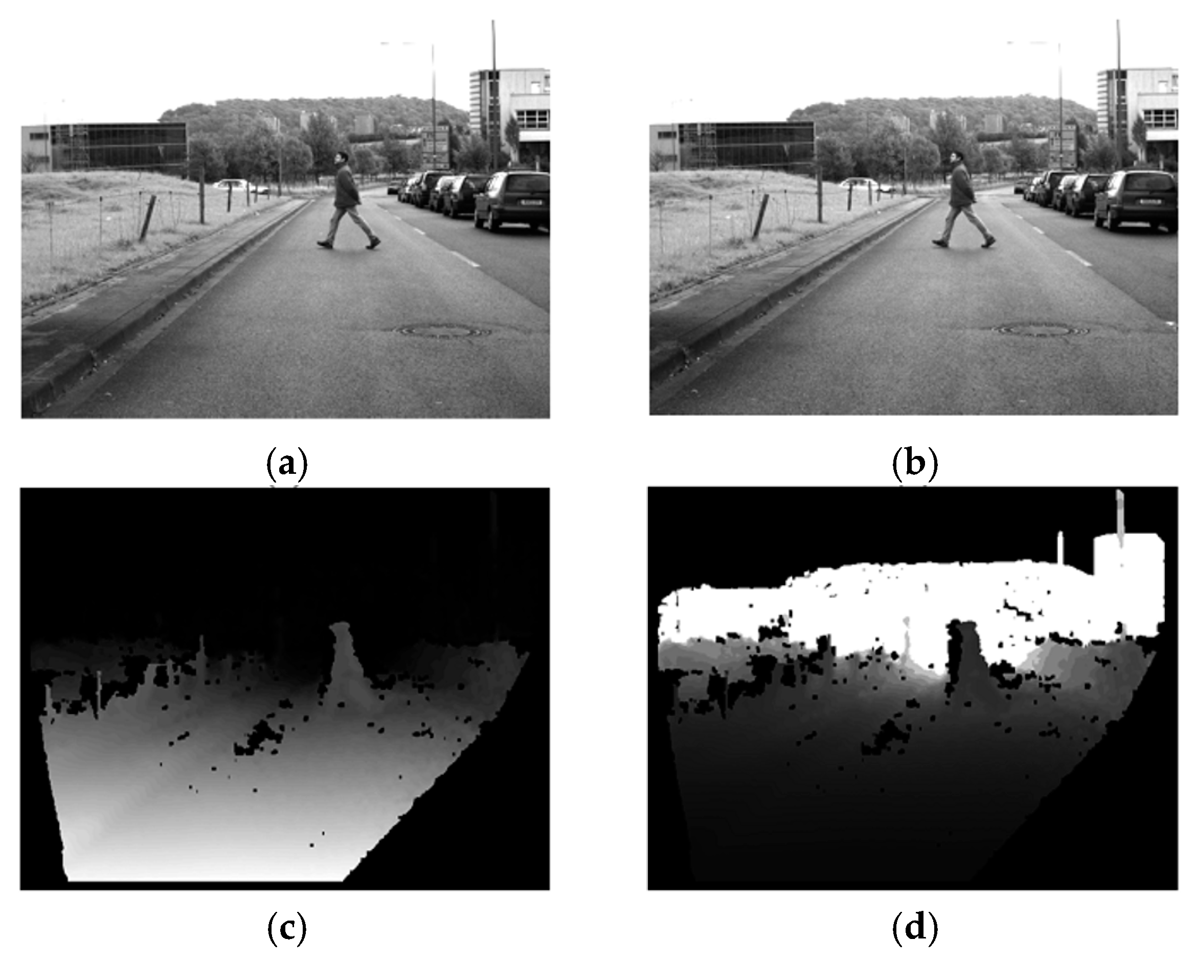
First, the disparity map is extracted from the calibrated stereo image using the Efficient Large-Scale Matching (ELAS) [15], which is one of the most commonly used stereo matching algorithms. It is the fastest and most accurate nonglobal stereo matching method among the algorithms using only Central Processing Unit (CPU) in the Middlebury dataset [16]. Figure 2c shows the disparity map extracted using ELAS. The object closer to the camera has a larger disparity, so it gets brighter in the disparity map. In the case of the road, the disparity value gradually decreases, as the distance from the camera increases.
The v-disparity map is a visualization of a histogram that accumulates the number of pixels having the same disparity in each row of the disparity map. Figure 3 shows the v-disparity map generated using the disparity map in Figure 2c. The rows of the v-disparity map represent rows of the disparity map. The column of the v-disparity map represents the disparity value, ranging from 0 to max disparity. The max disparity means the maximum search range when searching for corresponding pixels in a stereo image.
Images taken from a car contain more roads than objects such as trees, buildings, and cars. Therefore, the road appears in the form of a strong straight-line in the v-disparity map. If the equation of this line is known, the road can be estimated. We first apply two post-processing algorithms to this map to detect the straight-line. The first step is noise removal. In the v-disparity map, the noise is a pixel having a small value that interferes with the detection of the line. We regard pixels smaller than a threshold value as noise and remove it. The threshold is dependent on the resolution, and the proposed method effectively removes noise when the threshold is set to 100 for VGA video stream resolution. Since the road is generally located at the bottom of the image, a straight line corresponding to the road exists in the lower part of the v-disparity map. Therefore, we remove the upper half region of the v-disparity map and detect the straight-line using Hough transform [17]. A number of lines of similar shape that satisfy the v-disparity map are detected. We take a line with highest peak in the Hough space. The road is estimated using the equation of the straight line. When the disparity map is scanned from the upper left corner, the disparity value of the reference pixel and the y coordinate are determined to be the ground if they are included in the straight line. However, because there is an error in the disparity map, the threshold value is set as in Equation (2) in actual operation.
where Equation (1) is the detected straight-line equation, d′ is the disparity value of the current pixel, and y′ is the Y coordinate of the current pixel. t denotes the threshold value, and we set it to 3 in the proposed method. A pixel satisfying the Equation (2) is estimated as the ground. Figure 4 shows the results of road estimation, with the road area marked in green.
2.2. Depth Map Calculation
The disparity map is converted to a depth map using the camera’s focal length and the distance between the stereo cameras. Figure 5 shows the camera position and coordinate system in stereo vision, where xl and xr represent the coordinates of the left and right images, respectively. f represents the focal length of the camera. b is the distance between the cameras, and Z is the distance between the camera and the object.
In Figure 5, there is a triangle with vertex on the left-hand camera and object. Equation (3) is derived using the proportional expression in this triangle. Similarly, Equation (4) is derived using a triangle with the right-hand camera and object as vertices.
Substituting Equation (4) into Equation (3) leads to Equation (5). Converting the left term of Equation (5) to Z yields Equation (6), which converts the disparity value to the depth value.
where d is the disparity. Figure 2d shows the depth map. Since the image expresses the distance between the camera and the object, in contrast to the disparity map, the brightness value increases as the object moves away from the camera.
2.3. System Motion Estimation
We use optical flow to extract the motion vector and estimate the system motion [18]. The system motion is represented by linear motion and rotation motion in the X, Y, and Z-axis, and can be obtained using the SFM [13], as shown in Equation (7).
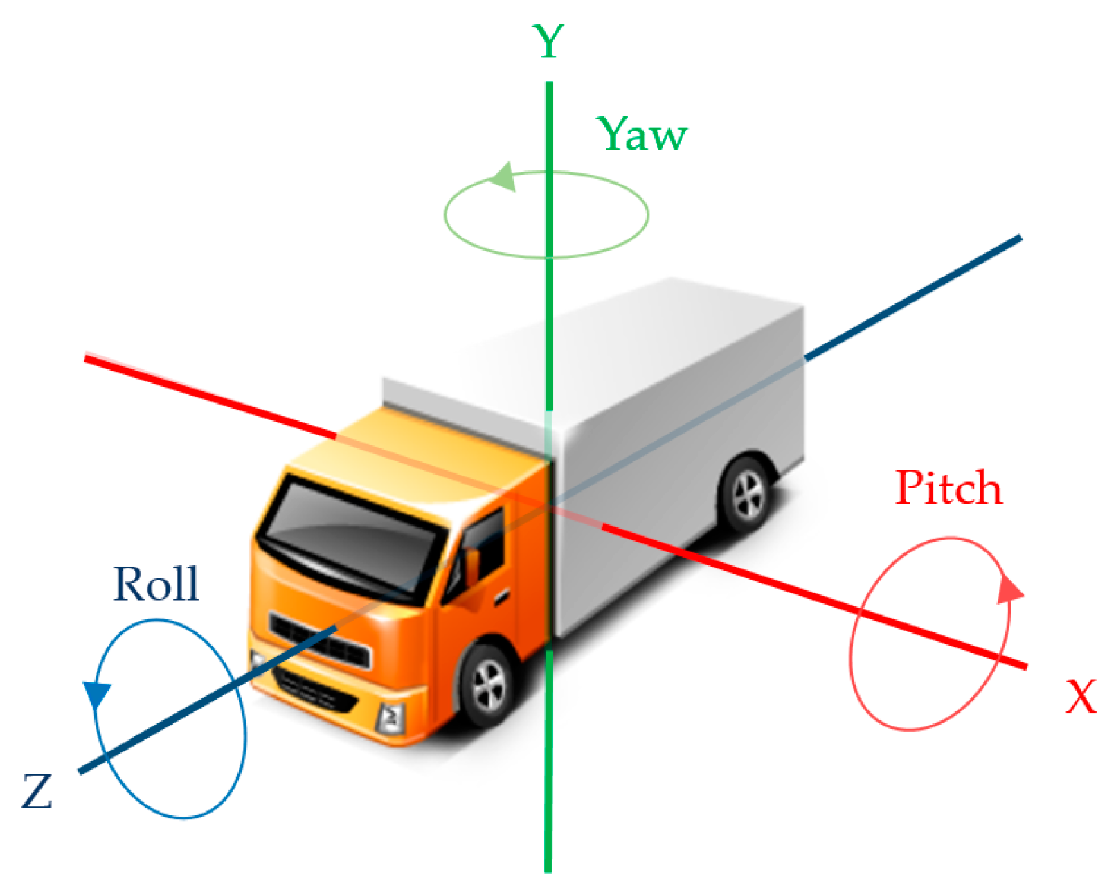
where x and y represent the coordinate of the image. u and v represent the motion vector for each coordinate. Tx, Ty, and Tz are the linear motion of the system. Wx, Wy, and Wz represent the rotating motion of the system and is called pitch, yaw, and roll, respectively. f is the focal length of the camera, and Z is the actual distance between the camera and the corresponding object.
Equation (7) has a large amount of computation, because it has six variables. Therefore, we transform Equation (7) by simplifying the motion of the car. Figure 6 shows the rotation and linear motion of the car on the X, Y, and Z axes. In case of airplane, it is necessary to consider rotational motion for all axes, but since the car is on the road, it is possible to define the movement of the car by the Z-axis linear motion and the X-axis rotation (pitch), and Y-axis rotation (yaw).
Equation (8) can be obtained by setting Tx, Ty, and Wz to zero in Equation (7). System motions Tz, Wx and Wy are obtained through inverse matrix computation.
However, the system motion cannot be obtained by the above process alone. The motion vectors are divided into two types: global vector and composite vector. The global vectors are generated by system motion, and are usually located on nonmoving objects such as trees and buildings. On the other hand, composite vectors occur under the influence of system and local motion, and are located in moving objects such as pedestrians and vehicles. If this is used in system motion calculations, it will cause incorrect results because the motion of the object is included. Therefore, we use RANSAC to exclude composite motion vectors and obtain the system motion that reflects global motion vectors. RANSAC can relatively estimate an accurate model even if some outliers exist in data, so it is suitable for our model that has a mixture of mostly global motion vectors and a few composite motion vectors. Figure 7 shows the process for estimating the system motion using RANSAC.
Since Equation (8) has three variables, three equations are needed to solve it. Therefore, three random motion vectors are extracted from the motion vectors, and the system motion, Tz, Wx and Wy are calculated by substituting the vectors into Equation (8). Since this system motion may reflect the composite motion vector, error calculation is necessary. The system motion is substituted into Equation (8), and the motion vectors u′ and v′ for error calculation are obtained at each pixel. The sum of absolute difference (SAD) between these motion vectors and the motion vectors obtained through the optical flow is calculated as shown in Equation (9).
where I represents all the pixels from which the motion vector has been extracted, and p represents one of them. u and v represent the motion vector extracted using the LK optical flow. The error e is the SAD value between the two vectors. The SAD value means the error of the system motion obtained from the randomly selected three motion vectors.
The above procedure is repeated until the error becomes smaller than emin. We set emin to 5 which showed the best performance in several experiments. Generally, the system motion can be obtained by repeating the process of Figure 7 about 1000 times. Figure 8a shows the extracted motion vectors using the LK optical flow, while Figure 8b shows the motion vectors calculated using the system motion acquired by the proposed method. Since the system motion is correctly estimated, it shows that the motion vectors of the two images do not differ greatly.
2.4. Moving Object Detection
We first detect all objects and determine whether each object moves. The object detection is performed through YOLO v3, an object detection algorithm based on deep learning. It shows the best performance in terms of speed vs. accuracy among related algorithms. The original YOLO v3 trained on Common Objects in COntext (COCO) dataset [19] with 172 categories. We trained YOLO v3 to detect only pedestrians and vehicles for our purpose.
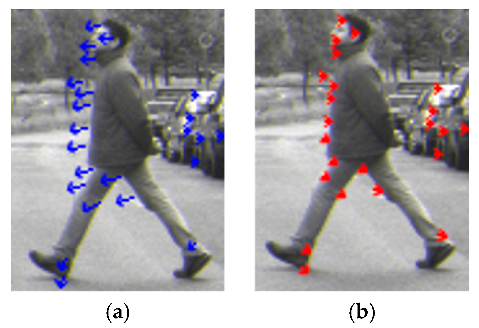
The determination of whether each object is moving is performed by comparing the motion vectors obtained by the optical flow with the motion vectors obtained using the system motion. Figure 8 shows these motion vectors on a moving object. Since the object moves from right to left, the motion vectors are also detected in the same direction as shown in Figure 9a. However, since the motion vector obtained by the system motion is generated only by the camera motion, it is represented in a form independent of the object motion as shown in Figure 9b.
Before comparing the two vectors, we first remove background, non-object areas, in the bounding box because it is not related to the motion of the object. We separated the foreground and background by applying image segmentation to the disparity map. A pixel whose absolute difference from the disparity value of the center pixel in the bounding box is larger than 5 is classified as background. Whether an object moves is determined through motion vector analysis of the foreground. However, some of the motion vectors obtained by the system motion are erroneous. This is because the disparity value extracted through stereo matching can generate an error. Therefore, a confidence measurement is required for each motion vector. The system motion for each motion vector is calculated using Equation (8). If the error between this and the previously acquired system motion is 10% or more, the corresponding motion vector is not used for object motion determination.
When comparing two vectors, angle and length are considered. A large error in the angle or size between the two vectors means that motion of the object is reflected in the motion vector obtained through the optical flow. We designed a method of measuring the error probability between the two vectors, each modelled as a Gaussian distribution as shown in Equation (10). The error probability represents the value with the highest probability considering the Gaussian distribution of size and angle difference between the vectors.
where s is the difference in size between motion vectors extracted from the optical flow and motion vectors obtained using the system motion. r represents the angle between the two vectors. σs and σr means the standard deviation of the angle and the size difference, respectively. The deviation is an acceptable value for the error, and if each value exceeds this deviation, the error will be increased. If the error probability is greater than 0.5, the vector extracted from the optical flow determines that the movement of the object was affected. This process is performed on all vectors within the object, and if 0.7 or more of the vectors are like this, it is judged to be moving objects. Additionally, for objects moving at the same speed as the camera, the motion vector extracted by the optical flow is small or zero. On the other hand, vectors calculated by system motion at the same position are independent of the motion of the object because the motion of the camera is compensated. Thus, the proposed method can also detect objects moving at the same speed as the system.
3. Experimental Results
We first performed experiments on the system motion extraction performance. The Daimler Stereo Pedestrian Detection Benchmark Dataset [20] was captured from a vehicle during a 20-min drive through urban traffic, at Video Graphics Array (VGA) resolution. The dataset consists of 16,401 stereo images, and provides baseline and focal length, camera-related parameters. In addition, this dataset provides ground truth for yaw rotation, which is suitable for the performance evaluation of system motion extraction. We tested it on a computer equipped with an Intel i7-7700K, 32GB RAM, and GTX 1080Ti. The Graphics Processing Unit (GPU) is only used when running YOLO. The speed of the proposed method depends on the number of detected objects, but on the Daimler dataset it takes 0.19 s on average per frame as shown in Table 1.
Figure 10 compares the system motion extracted by the proposed method, and the ground truth. The X-axis of the graph is the frame number, and the Y-axis is yaw rate. If the yaw rate is positive, it is clockwise rotation. Since the Daimler dataset has large capacity, only the first 500 frames were tested. A relatively high yaw value at about the 50th frame means that the car is turning a lot in the clockwise direction. A yaw value close to zero at about the 100th frame means that the car is going straight. The proposed method shows only a little noise, and not much difference compared with the ground truth.
To evaluate the accuracy of the proposed method, we compared it with two related works [6,11]. We set the cell size of the optical flow to 14 × 14 in [6]. We set the threshold for forward-backward error to 2 and the number of iterations for RANSAC to 1000 in [11]. Figure 11 shows a graph of Yaw errors for each method. The x-axis of the graph represents the number of frames of the Daimler dataset, and the y-axis represents the Yaw error. For the quantitative evaluation, the average of the error of each method is calculated in the graph. The Yaw-error value of the proposed method is 0.00471, which is about 0.003 lower than the other methods.
Table 2 shows the average of the difference between the result and the ground truth for each method. In this experiment, we used all frames of the Daimler dataset instead of using 500 frames, as in previous experiments. The Yaw error of the proposed method is 0.00471, which is about 40% less than that of [11]. We consider that extracting the system motion after removing the road in the proposed method contributes to the performance increase.
To evaluate the detection of moving objects, we experimented with two datasets. The first one is the Daimler dataset that we have used in previous experiments, and we manually detected the moving object, because there is no label for the moving object. The second one was taken directly after installing the stereo camera as shown in Figure 12. The camera is Point Gray’s Flea USB 3.0 model with a resolution of 1280 by 1024. A total of 25 min of data collection was taken around the university, and the labeling of moving objects was done manually as well. Table 3 shows the details for each dataset.
Figure 13 shows the result of applying the proposed method to the Daimler dataset. In Figure 13a,b, a car is on the side, but is not detected, because it does not move. On the other hand, one person in the center of the image is detected, because the person is moving from right to left. Similarly, in Figure 13c,d, the vehicle that is stationary is not detected, but only the moving one is detected.
Table 4 compares the performance of each method for moving object detection on the Daimler dataset. We compare the proposed method with three related works, [6,8,21]. In [8], we fine-tuned the constant parameter α to 2.0, which is used when summing superpixels. In the [21], motion likelihood at each pixel is estimated by considering ego-motion and disparity. Then, a graph-cut based algorithm is used to remove a pixel with the false likelihood by considering both the color and disparity information. Finally, the bounding boxes are generated for each moving object by using the UV-disparity map. We fine-tuned the parameters σ and γ, which are used when computing the variance of disparity, to 0.2 and 0.065, respectively. In the table, true positive is the correct detection of a moving object. False positive is the detection of a static object. False negative means moving object, but not detected. Compared with [8], the proposed method has 13 more true positives among 240 moving object ground truths, and 6 and 8 less false positives and false negatives, respectively. Compared with [6], it has 36 more true positive numbers, and 13 less false positives and 15 less false negatives, respectively. Compared with [21], it has 11 less true positive numbers, and 11 less false positives and 2 more false negatives, respectively. In addition, we calculated the precision, recall, and F-measure of each method using Equation (11).
Compared with [8], the precision, recall, and F-measure are 2.83%, 3.58% and 3.22% higher, respectively. Compared with [6], the precision, recall, and F-measure are 6.79%, 7.65% and 7.24% higher, respectively. Compared with [21], the precision, and F-measure are 3.89 %, and 1.37% higher, respectively but the recall is 1.1% lower.
Table 5 shows performance comparisons for moving object detection in our dataset. Compared with [8], the proposed method has 10 more true positive numbers, and 4 less false positive numbers and 11 less false negative numbers, respectively. Compared with [6], it has 26 more true positive numbers, and 17 less false positives and 23 less false negatives, respectively. Compared with [21], it has 7 less true positive numbers, and 9 less false positives and 5 less false negatives, respectively.
Compared with [8], the precision, recall and F-measure are 0.98%, 2.44%, and 1.72% higher, respectively. Compared with [6], the precision, recall and F-measure are 4.01%, 5.22%, 4.62% higher, respectively. Compared with [21], the precision, recall and F-measure are 1.81%, 0.95%, 1.38% higher, respectively.
4. Conclusions
In this paper, we propose a method to detect moving objects using a stereo camera in a car. First, we improved the accuracy of the system motion by removing the road using the v-disparity map. Additionally, RASNAC was used to improve the accuracy of system motion. We detected the object by the deep learning-based network, and detected the moving object using the error reliability measures modeled as Gaussian distributions. The experimental results show that the proposed method outperforms other related methods on various datasets.
Author Contributions
Conceptualization, G.-c.L.; Methodology, J.Y.; Software, G.-c.L.; Investigation, G.-c.L.; Writing—Original Draft Preparation, G.-c.L.; Writing—Review & Editing, J.Y.; Supervision, J.Y.; Project Administration, J.Y.
Funding
This research received no external funding.
Acknowledgments
The work reported in this paper was conducted during the sabbatical year of Kwangwoon University in 2017.
Conflicts of Interest
The authors declare no conflicts of interest.
References
- Huval, B.; Wang, T.; Tandon, S.; Kiske, J.; Song, W.; Pazhayampallil, J.; Andriluka, M.; Rajpukar, P.; Migimatsu, T.; Cheng-Yue, R.; et al. An empirical evaluation of deep learning on highway driving. arXiv, 2015; arXiv:1504.01716v3. [Google Scholar]
- Gavrila, D.M. Sensor-based pedestrian protection. IEEE Intell. Syst. 2001, 16, 77–81. [Google Scholar] [CrossRef]
- Gopalakrishnan, S. A public health perspective of road traffic accidents. J. Fam. Med. Prim. Care 2012, 1, 144–150. [Google Scholar] [CrossRef] [PubMed]
- Piccardi, M. Background subtraction techniques: A review. In Proceedings of the 2004 IEEE International Conference on Systems, Man and Cybernetics, The Hague, The Netherlands, 10–13 October 2004. [Google Scholar]
- Postica, G.; Romanoni, A.; Matteucci, M. Robust moving objects detection in lidar data exploiting visual cues. In Proceedings of the IEEE/RSJ International Conference on Intelligent Robots and Systems (IROS), Daejeon, Korea, 9–14 October 2016. [Google Scholar]
- Hariyono, J.; Hoang, V.D.; Jo, K.H. Moving object localization using optical flow for pedestrian detection from a moving vehicle. Sci. World J. 2014, 2014, 1–8. [Google Scholar] [CrossRef] [PubMed]
- Bouguet, J.Y. Pyramidal implementation of the affine lucas kanade feature tracker description of the algorithm. Intel Corp. 2001, 5, 1–10. [Google Scholar]
- Chen, L.; Fan, L.; Xie, G.; Huang, K.; Nuchter, A. Moving-object detection from consecutive stereo pairs using slanted plane smoothing. IEEE Trans. Intell. Transp. Syst. 2017, 18, 3093–3102. [Google Scholar] [CrossRef]
- Kitt, B.; Geiger, A.; Lategahn, H. Visual odometry based on stereo image sequences with ransac-based outlier rejection scheme. In Proceedings of the IEEE Intelligent Vehicles Symposium, San Diego, CA, USA, 21–24 June 2010. [Google Scholar]
- Achanta, R.; Shaji, A.; Smith, K.; Lucchi, A.; Fua, P.; Susstrunk, S. SLIC superpixels compared to state-of-the-art superpixel methods. IEEE Trans. Pattern Anal. Mach. Intell. 2012, 34, 2274–2282. [Google Scholar] [CrossRef] [PubMed]
- Seo, S.W.; Lee, G.C.; Yoo, J.S. Motion Field Estimation Using U-Disparity Map in Vehicle Environment. J. Electr. Eng. Technol. 2017, 12, 428–435. [Google Scholar] [CrossRef] [Green Version]
- Labayrade, R.; Aubert, D.; Tarel, J.P. Real time obstacle detection in stereovision on non flat road geometry through v-disparity representation. In Proceedings of the IEEE Intelligent Vehicle Symposium, Versailles, France, 17–21 June 2002. [Google Scholar]
- Turner, D.; Lucieer, A.; Watson, C. An automated technique for generating georectified mosaics from ultra-high resolution unmanned aerial vehicle (UAV) imagery, based on structure from motion (SfM) point clouds. Remote Sens. 2012, 4, 1392–1410. [Google Scholar] [CrossRef]
- Redmon, J.; Divvala, S.; Girshick, R.; Farhadi, A. You only look once: Unified, real-time object detection. In Proceedings of the IEEE Conference on Computer Vision and Pattern Recognition (CVPR 2016), Las Vegas, NV, USA, 27–30 June 2016. [Google Scholar]
- Geiger, A.; Roser, M.; Urtasun, R. Efficient large-scale stereo matching. In Proceedings of the Asian Conference on Computer Vision (ACCV 2010), Queenstown, New Zealand, 8–12 November 2010. [Google Scholar]
- Scharstein, D.; Pal, C. Learning conditional random fields for stereo. In Proceedings of the IEEE Computer Society Conference on Computer Vision and Pattern Recognition (CVPR 2007), Minneapolis, MN, USA, 17–22 June 2007. [Google Scholar]
- Ballard, D.H. Generalizing the Hough transform to detect arbitrary shapes. Pattern Recognit. 1981, 13, 111–122. [Google Scholar] [CrossRef] [Green Version]
- Giachetti, A.; Campani, M.; Torre, V. The use of optical flow for road navigation. IEEE Trans. Robot. Autom. 1998, 14, 34–48. [Google Scholar] [CrossRef] [Green Version]
- Lin, T.Y.; Maire, M.; Belongie, S.; Hays, J.; Perona, P.; Ramanan, D.; Dollár, P.; Lawrence Zitnick, C. Microsoft coco: Common objects in context. In Proceedings of the 13th European Conference on Computer Vision (ECCV 2014), Zurich, Switzerland, 6–12 September 2014. [Google Scholar]
- Keller, C.; Enzweiler, M.; Gavrila, D.M. A New Benchmark for Stereo-based Pedestrian Detection. In Proceedings of the IEEE Intelligent Vehicles Symposium, Baden-Baden, Germany, 5–9 June 2011. [Google Scholar]
- Zhou, D.; Frémont, V.; Quost, B.; Dai, Y.; Li, H. Moving object detection and segmentation in urban environments from a moving platform. Image Vis. Comput. 2017, 68, 76–87. [Google Scholar] [CrossRef] [Green Version]
Figure 1.
Flowchart of the proposed method.

Figure 2.
Disparity map extraction using Efficient Large-Scale Matching (ELAS): (a) left image, (b) right image, (c) disparity image, and (d) depth image.
Figure 2.
Disparity map extraction using Efficient Large-Scale Matching (ELAS): (a) left image, (b) right image, (c) disparity image, and (d) depth image.

Figure 3.
V-disparity map generation.

Figure 4.
Result of road estimation.

Figure 5.
Camera position and coordinate system for stereo vision.

Figure 6.
Motion of a car.

Figure 7.
Process for estimating global motion using RANSAC.

Figure 8.
Motion vector comparison. (a) Motion vector acquired using optical flow, and (b) motion vector acquired using system motion.
Figure 8.
Motion vector comparison. (a) Motion vector acquired using optical flow, and (b) motion vector acquired using system motion.

Figure 9.
The motion vector of the moving object. (a) Motion vector extracted by the Lucas-Kanade (LK) optical flow, and (b) motion vector calculated using system motion.
Figure 9.
The motion vector of the moving object. (a) Motion vector extracted by the Lucas-Kanade (LK) optical flow, and (b) motion vector calculated using system motion.

Figure 10.
System motion performance comparison between the proposed method and the ground truth.

Figure 11.
Yaw error comparison on the Daimler dataset.

Figure 12.
Experimental environment of our dataset. (a) Setting 1, and (b) Setting 2.

Figure 13.
The result of applying the proposed method to the Daimler dataset. (a) Result image 1, (b) Result image 2, (c) Result image 3, and (d) Result image 4.
Figure 13.
The result of applying the proposed method to the Daimler dataset. (a) Result image 1, (b) Result image 2, (c) Result image 3, and (d) Result image 4.


Table 1.
Processing time of each part of the proposed method.
| Algorithm | Processing Time (ms) |
|---|---|
| Stereo matching (ELAS [15]) | 73 |
| Road estimation | 1 |
| System motion estimation | 97 |
| Object detection (YOLO [14]) | 17 |
| Moving object detection | 2 |
| Total | 190 |
Table 2.
Performance comparison for system motion extraction.
| Method | Yaw Error (degree/s) |
|---|---|
| The proposed method | 0.00471 |
| Hariyono’s method [6] | 0.00781 |
| Seo’s method [11] | 0.00779 |
Table 3.
Specification of each dataset used in the experiment.
| Dataset | Frames | Moving Objects | Static Objects |
|---|---|---|---|
| Daimler dataset | 22,500 | 437 | 794 |
| Our dataset | 12,000 | 240 | 545 |
Table 4.
Comparison experiment result on Daimler dataset.
| Method | True Positive | False Positive | False Negative | Precision | Recall | F-Measure |
|---|---|---|---|---|---|---|
| Proposed method | 220 | 12 | 20 | 0.9483 | 0.9167 | 0.9322 |
| Chen’s method [8] | 207 | 18 | 28 | 0.9200 | 0.8809 | 0.9000 |
| Hariyono’s method [6] | 184 | 25 | 35 | 0.8804 | 0.8402 | 0.8598 |
| Zhou’s method [21] | 231 | 23 | 18 | 0.9094 | 0.9277 | 0.9185 |
© 2019 by the authors. Licensee MDPI, Basel, Switzerland. This article is an open access article distributed under the terms and conditions of the Creative Commons Attribution (CC BY) license (http://creativecommons.org/licenses/by/4.0/).
Share and Cite
MDPI and ACS Style
Yoo, J.; Lee, G.-c. Moving Object Detection Using an Object Motion Reflection Model of Motion Vectors. Symmetry 2019, 11, 34. https://doi.org/10.3390/sym11010034
AMA Style
Yoo J, Lee G-c. Moving Object Detection Using an Object Motion Reflection Model of Motion Vectors. Symmetry. 2019; 11(1):34. https://doi.org/10.3390/sym11010034
Chicago/Turabian StyleYoo, Jisang, and Gyu-cheol Lee. 2019. "Moving Object Detection Using an Object Motion Reflection Model of Motion Vectors" Symmetry 11, no. 1: 34. https://doi.org/10.3390/sym11010034
Note that from the first issue of 2016, this journal uses article numbers instead of page numbers. See further details here.