An Improved Integer Transform Combining with an Irregular Block Partition

Abstract

After conducting deep research on all existing reversible data hiding (RDH) methods based on Alattar’s integer transform, we discover that the frequently-used method in obtaining the difference value list of an image block may lead to high embedding distortion. To this end, we propose an improved Alattar’s transform-based-RDH-method. Firstly, the irregular block partition method which makes full use of high correlation between two neighboring pixels is proposed to increase the embedding performance. Specifically, each image block is composed of a center pixel and several pixels surrounding this center pixel. Thus, the difference value list is created by using the center pixel to predict each pixel surrounding it. Since the center pixel is highly related to each pixel surrounding it, a sharp difference value histogram is generated. Secondly, the mean value of an image block in Alattar’s integer transform has embedding invariance property, and therefore, it can be used for increasing the estimation performance of a block’s local complexity. Finally, two-layer embedding is combined into our scheme in order to optimize the embedding performance. Experimental results show that our method is effective.

1. Introduction

In the field of information security, a technique called data hiding has been developed widely to hide secret bits into cover images for copyright protection, image authentication, etc. However, most data hiding techniques only focus on correct extraction of hidden data, while neglect lossless recovery of cover images. It is known that lossless recovery of cover images is required in some applications like remote sensing, law enforcement, archive management, etc. Thus, reversible data hiding (RDH), a kind of special data hiding, is presented to satisfy the requirements of these applications. Its speciality lies in the fact that it enables the original image to be completely recovered without any distortion after the embedded bits are extracted.

In the past decade, RDH has been extensively studied and a large amount of RDH schemes have been proposed. Here, we categorize the existing RDH schemes into five main classes according to their used techniques: lossless compression [1], difference expansion (DE) [2], histogram shifting (HS) [3], prediction-error expansion (PEE) [4] and integer transform [5,6,7,8]. In the early stage of RDH development, lossless compression was the frequently-used technique, in which secret bits are embedded into the vacant embedding space generated by compressing the images. However, lossless compression cannot provide high embedding capacity. The demand for high embedding capacity was becoming more and more urgent. In 2003, Tian proposed an RDH method called DE to make a great improvement in embedding capacity [2]. The key idea of schemes based on DE is to expand the difference value between two adjacent pixels to create a vacant least significant bit (LSB), and then embed one data bit into this empty LSB. HS was firstly proposed by Ni et al. to select the maximum and minimum points in the histogram for embedding [9]. The maximum modification in HS is one grayscale unit. Afterwards, some improvements on HS were generated [10]. After studying DE deeply, Thodi et al. found that DE can be further improved to obtain a sharper difference histogram. To this end, Thodi et al. introduced the prediction in DE, and thus a sharper prediction-error histogram is generated, which helps to further improve embedding performance. Later, various research on how to improve the prediction accuracy has been carried out [11,12,13,14,15,16,17,18,19,20,21,22,23,24,25]. The schemes based on integer transform have a similar feature that more than two pixels are grouped into a unit, and then this unit is processed to carry data via an integer transform [5,6,7,8].

Compared with Alattar’s transform [5], Weng et al.’s method [8] selects previously the blocks located in smooth regions for data embedding. Therefore, the smoothness estimation of blocks is very important to the increase of embedding performance. Alattar’s method has a characteristic that the mean value of a block is kept unaltered after embedding. Weng et al. made full use of this characteristic and utilized the mean value of a block along with pixels surrounding this block to estimate a block’s smoothness. Thus, the application of the invariant mean value helps to increase embedding performance. In Weng et al.’s method, there is still room for improvement. They obtain the difference list by calculating the difference values between every two neighboring pixels in a block. Since two neighboring pixels are highly related, a sharp distribution of difference histogram is generated. However, in the process of calculating the watermarked pixels, they neglect that the accumulated sum of difference values is very large, and cannot be ignored, especially when most difference values within a block are positive integers or most difference values within a block are negative integers. More importantly, the accumulated sum results in large modifications to the original pixels. That is to say, the difference between the original and hidden pixels is very large. As an extension of Weng et al.’s method, we propose an improved Alattar’s transform-based-RDH-method. Firstly, the irregular block partition method which makes full use of high correlation between two neighboring pixels on the basis of reducing embedding distortion is proposed. Specifically, each image block is composed of a center pixel and its surrounding pixels. Thus, the difference value list is created by using the center pixel to predict each pixel surrounding it. Since the center pixel is highly related to its surrounding pixels, a sharp difference value histogram is generated. Secondly, the mean value of an image block in Alattar’s integer transform has embedding invariance property, and, therefore, it can be used for increasing the estimation performance of block’s local complexity. Finally, two-layer embedding is combined into our scheme in order to optimize the embedding performance. Extensive experimental results show that the proposed method has better embedding performance.

2. Related Works

2.1. Weng et al.’s Method

Here, we will give a simple introduction for Weng et al.’s method. In their method, the original image I is partitioned into non-overlapped image blocks with size n. All the pixels in a block are arranged into a one-dimensional pixel list $\mathbf{x}$ according to odd rows from left to right, even rows from right to left (see Figure 1). The mean value $\overline{x}$ of $\mathbf{x}$ and the $n-1$ difference values can be calculated as Equation (1):

$$\begin{array}{lll}\overline{x}& =& \frac{x_1+x_2+\dots +x_n}{n},\\ d_1& =& x_2-x_1,\\ d_2& =& x_3-x_2,\\ \dots \\ d_{n-1}& =& x_n-x_{n-1},\end{array}$$

(1)

where $x_1,x_2,\dots ,x_{n-1},x_n$ are n pixels of the pixel list $\mathbf{x}$, and $\overline{x}$ is the mean value of $\mathbf{x}$.

Figure 1. Taking a $4\times 4$-sized block for example, a two-dimensional image block is arranged into a one-dimensional pixel list according to the arrow direction.

The inverse transform of Equation (1) is formulated in Equation (2):

$$\begin{array}{lll}{y}_1& =& ⌊\overline{x}⌋-⌊\frac{(n-1)\times d_1+(n-2)\times d_2+\dots +d_{n-1}}{n}⌋,\\ y_2& =& y_1+d_1,\\ y_3& =& y_2+d_2,\\ \dots \\ y_n& =& y_{n-1}+d_{n-1},\end{array}$$

(2)

where $\mathbf{y}=\left\{y_1,y_2,\dots ,y_{n-1},y_n\right\}$ represents the watermarked pixel list. From Equation (2), we know the difference value $d_i$, $i\in \{1,\dots ,n-1\}$, is magnified by $n-i$ times in the process of calculating $y_1$ when $d_i$ is generated by two neighboring pixels. This is also the reason that the difference values calculated by every two neighboring pixels would result in high embedding distortion. The rest of this section will explain it.

If each of $n-1$ difference values is expanded to carry one-bit data, then Equation (2) can be converted into Equation (3):

$$\begin{array}{lll}{y}_1& =& ⌊\overline{x}⌋-⌊\frac{(n-1)\times \left(2(x_2-x_1)+w_1\right)+(n-2)\times \left(2(x_3-x_2)+w_2\right)+\dots +\left(2(x_n-x_{n-1})+w_{n-1}\right)}{n}⌋,\\ & =& ⌊\overline{x}⌋-⌊\frac{2{\displaystyle \sum _{\mathrm{i}=1}^{\mathrm{n}}}{x}_i+{\displaystyle \sum _{i=1}^{\mathrm{n}-1}}(\mathrm{n}-\mathrm{i})\times {\mathrm{w}}_{\mathrm{i}}-2n\times x_1}{n}⌋,\\ y_2& =& y_1+2\times d_1+w_1=y_1+2(x_2-x_1)+w_1,\\ y_3& =& y_2+2\times d_2+w_2=y_2+2(x_3-x_2)+w_2,\\ \dots \\ y_{n-1}& =& y_{n-2}+2\times d_{n-2}+w_{n-2}=y_{n-2}+2(x_{n-1}-x_{n-2})+w_{n-2},\\ y_n& =& y_{n-1}+2\times d_{n-1}+w_{n-1}=y_{n-1}+2(x_n-x_{n-1})+w_{n-1}.\end{array}$$

(3)

In order to illustrate the effect of difference expansion on embedding distortion, Equation (3) needs to be further simplified. To this end, suppose $k_2={\displaystyle \sum _{i=1}^n}{x}_i-n⌊\overline{x}⌋$; then, we know $k_2\in \left\{0,1,\dots ,n-1\right\}$. ${\displaystyle \sum _{i=1}^n}{x}_i$ is replaced by $k_2+n⌊\overline{x}⌋$ to simplify Equation (3) as below:

$$\begin{array}{lll}{y}_1& =& ⌊\overline{x}⌋+2(x_1-⌊\overline{x}⌋)-A_t,\\ y_2& =& ⌊\overline{x}⌋+2(x_2-⌊\overline{x}⌋)+w_1-A_t,\\ y_3& =& ⌊\overline{x}⌋+2(x_3-⌊\overline{x}⌋)+w_2-A_t,\\ \dots \\ y_n& =& ⌊\overline{x}⌋+2(x_n-⌊\overline{x}⌋)+w_{n-1}-A_t,\end{array}$$

(4)

where the notation $A_t$ is used to denote an additional term, i.e., $A_t=$ $\lfloor \frac{(2k_2+{\displaystyle \sum _{i=1}^{\mathrm{n}-1}}\left(\mathrm{n}-\mathrm{i}\right)\times {\mathrm{w}}_{\mathrm{i}})}{n}\rfloor$.

After simplicity, it can be seen clearly that Equation (4) is composed of two parts: an embedding process and an additional term $A_t$. In the embedding process, $⌊\overline{x}⌋$ is regarded as a prediction value to predict each pixel within a block. The value of $A_t$ is related to the distortion (i.e., the modified magnitude of each pixel in $\mathbf{x}$. From the formula of calculating $A_t$, we know $A_t$ is mainly determined by $w_i$ and $k_2$, where $i\in \{1,2,\dots ,n-1\}$. In the rest of this paper, for simplicity of description, the range of the value i will be no longer rementioned. Specifically, since $k_2\in \left\{0,1,\dots ,n-1\right\}$ and $w_i\in \{0,1\}$, $0\le A_t\le ⌊\frac{2(n-1)+(n-1)+(n-2)+\dots +1}{n}⌋=⌊\frac{n+4}{2}(1-\frac{1}{n})⌋$. The maximum $⌊\frac{n+4}{2}(1-\frac{1}{n})⌋$ is obtained when $k_2$ is $n-1$ and all to-be-embedded bits are 1. Even if $A_t$ does not reach this maximum, $A_t$ is also very large because the $w_i$ is magnified by $n-i$ times. This maximum is determined predominantly by the block size n. In a word, the bigger the block size n is, the larger $A_t$ is, and the higher the distortion becomes.

According to the description above, blocks with large size n cannot be used in Weng et al.’s method. Therefore, the blocks with size 4 are utilized in their method. However, even if n is set 4, this maximum of $A_t$ is 3, which would still lead to large decline in PSNR value. In addition, when n is 4, the maximum embedding rate only reaches 0.75 bpp (bit per pixel). In other words, there is still much room for improvement in Weng et al.’s method. To this end, our method focuses on increasing block size on the basis of reducing embedding distortion as much as possible by adopting a different way of obtaining the difference values.

2.2. Alattar’s Method

Alattar’s integer transform can be formulated in Equation (5):

$$\begin{array}{lll}l& =& ⌊\frac{x_1+x_2+\dots +x_n}{n}⌋,\\ h_1& =& x_2-x_1,\\ h_2& =& x_3-x_1,\\ \dots \\ h_{n-1}& =& x_n-x_1,\end{array}$$

(5)

where the notation l is used to represent the average value of an n-sized image block, and $h_1,h_2,\dots ,h_{n-1}$ are $n-1$ difference values of this block.

In the data embedding process, the watermarked $h_j^{\prime }$ is obtained by expanding $h_j$ to carry 1-bit data, i.e., $h_j^{\prime }$ = 2$h_j$+$w_j$, where $j\in \{1,2,\dots ,n-1\}$. The watermarked pixels $y_1,\dots ,y_n$ are calculated via Equation (6):

$$\begin{array}{lll}{y}_1& =& l-⌊\frac{h_1^{\prime }+h_2^{\prime }+\dots +h_{n-1}^{\prime }}{n}⌋,\\ y_2& =& y_1+h_1^{\prime },\\ y_3& =& y_1+h_2^{\prime },\\ \dots \\ y_n& =& y_1+h_{n-1}^{\prime }.\end{array}$$

(6)

On the decoding side, the original difference $h_j$ is retrieved and the $w_j$ is extracted by Equation (7):

$$\begin{array}{lll}{h}_j& =& ⌊\frac{y_j-y_1}{2}⌋,\\ w_j& =& y_j-y_1-2h_j,\end{array}$$

(7)

where $j\in \{1,2,\dots ,n-1\}$.

Depending on the invariant l, the original pixels $x_1,x_2,\dots ,x_n$ are retrieved by the inverse integer transform of Equation (5) (i.e., Equation (8)):

$$\begin{array}{lll}{x}_1& =& l-⌊\frac{h_1+h_2+\dots +h_{n-1}}{n}⌋,\\ x_2& =& x_1+h_1,\\ \dots \\ x_n& =& x_1+h_{n-1}.\end{array}$$

(8)

3. The Proposed Scheme

According to the description in Section 2, the difference values created by two neighboring pixels would result in large embedding distortion. To resolve this problem, we need to change the way of obtaining difference values. However, in order to remain high visual quality, high correlation between two adjacent pixels needs to be preserved. To achieve this goal, an irregular block partition strategy is proposed in our method, in which each block is composed of a center pixel and its neighboring pixels. With the adoption of the irregular block partition strategy, the center pixel is adjacent to each pixel surrounding it. After block partition, the center pixel is utilized to predict each pixel surrounding it, so that a sharp prediction-error histogram is generated. Finally, two-layer embedding is utilized to further increase embedding performance. Here, we will give a detailed description for each part of the proposed method (i.e., irregular block partition, block selection and two-layer embedding), and, meanwhile, performance analysis in Section 3.2 is used to explain the reason that our method can achieve better performance than Weng et al.’s.

3.1. Irregular Block Partition

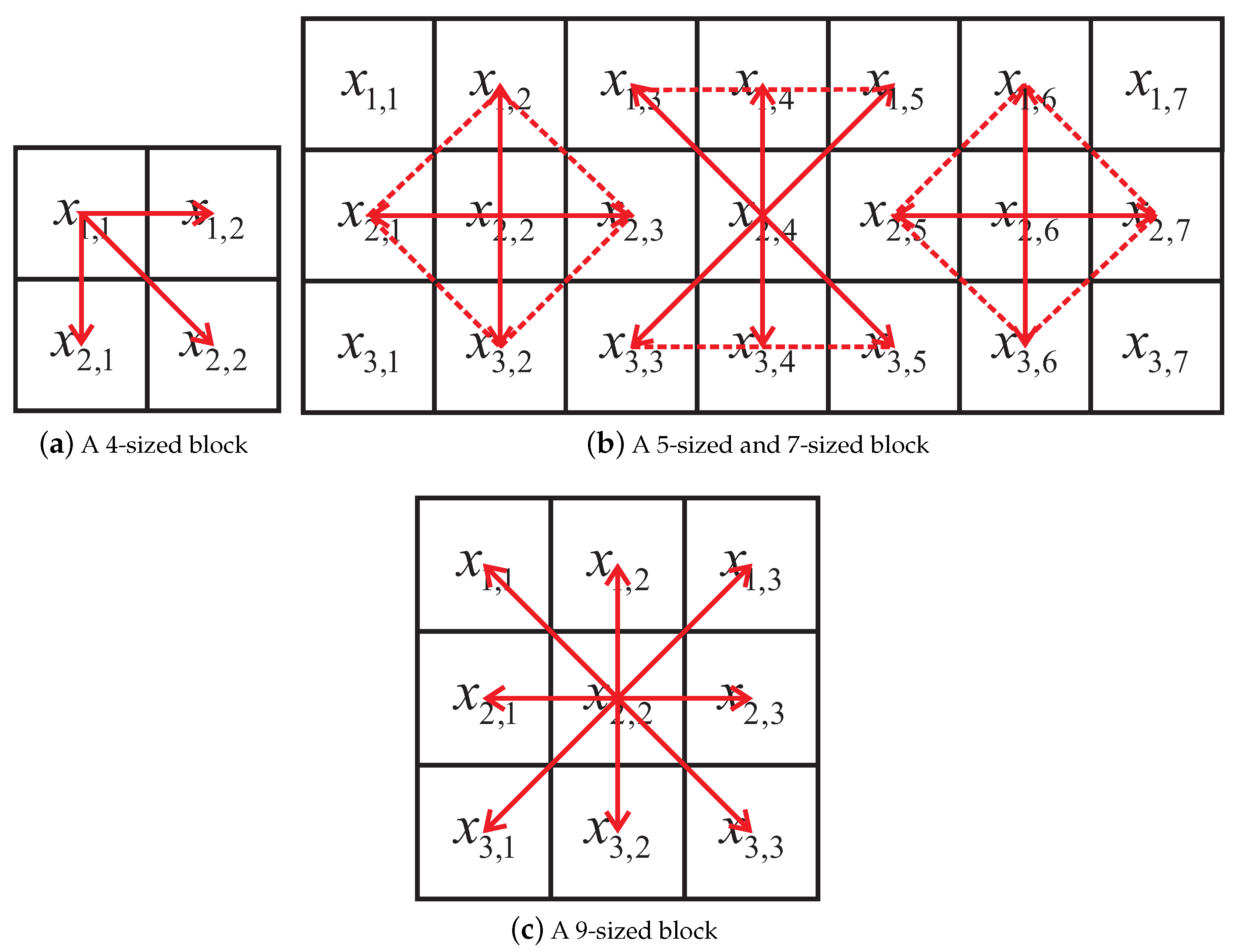
The key idea of constructing the irregular block partition is to design different partition methods for different sized blocks to increase the correlation between the center pixel and its neighbors. In our scheme, an n-sized block has its own particular partition strategy, and each block has a center pixel and its surrounding pixels, as shown in Figure 2. For a 4-sized image block, $x_{1,1}$ is the center pixel, and $x_{1,2}$, $x_{2,1}$ and $x_{2,2}$ are the three surrounding pixels of $x_{1,1}$ (Figure 2a). The blocks can also be a combination of 5-sized and 7-sized blocks (Figure 2b). In the rest of this paper, for simplicity, we utilize $n=5$ to indicate the block partition in Figure 2b. For a 9-sized block, the center pixel $x_{2,2}$ is surrounded by eight neighboring pixels (Figure 2c).

Figure 2. Various-sized image blocks.

In fact, our method can also be used for a generic block size n. However, the embedding performance may lead to an unsatisfactory result. To this end, we propose the irregular block partition. From Figure 2, one can observe that all three partition methods can make full use of high correlation between the center pixel and its neighboring pixels so that optimal embedding performance can be achieved. For an image I of a given size, it is partitioned into non-overlapped blocks according to one of three partition methods in Figure 2. Each partition method will yield a highest PSNR at a given payload. Therefore, there are three candidates of the PSNR. Among these three candidates, the highest PSNR is decided as the final PSNR. Meanwhile, the block partition method corresponding to the highest PSNR is selected as the optimal block size.

3.2. Performance Analysis

After block partition, for an n-sized (e.g., 4, 5 or 9) image block, the center pixel $x_c$ is used to predict each pixel surrounding $x_c$ so that the $n-1$ difference values $d_1,d_2,\dots ,d_{n-1}$ are generated:

$$\begin{array}{lll}\overline{x}& =& \frac{x_c+x_2+\dots +x_n}{n},\\ d_1& =& x_2-x_c,\\ d_2& =& x_3-x_c,\\ \dots \\ d_{n-1}& =& x_n-x_c.\end{array}$$

(9)

The inverse transform of Equation (9) is calculated in Equation (10):

$$\begin{array}{lll}{x}_c& =& \lfloor \overline{x}\rfloor -⌊\frac{d_1+d_2+\dots +d_{n-1}}{n}⌋,\\ x_2& =& x_c+d_1,\\ x_3& =& x_c+d_2,\\ \dots \\ x_n& =& x_c+d_{n-1}.\end{array}$$

(10)

During the embedding process, each original difference value is compared with a predefined threshold value $p{T}_h$ so as to determine its corresponding modification method. Specifically, if one difference value falls into $\left[-p{T}_h,p{T}_h\right)$, then it is suitable for expansion and it can be embedded with one-bit data. Otherwise, it is shifted by $p{T}_h$ to reduce embedding distortion (see Equation (11)):

$$d_k^{\prime }=\left\{\begin{array}{l}2\times d_k+b,d_k\in \left[-p{T}_h,p{T}_h\right),\\ d_k-p{T}_h,d_k\in \left(-\infty ,-p{T}_h-1\right],\\ d_k+p{T}_h,d_k\in \left[p{T}_h,+\infty \right).\end{array}\right.$$

(11)

Substitute all modified difference values in Equation (11) into Equation (10), and a watermarked pixel array $\mathrm{y}=\left\{y_c,y_2,\dots ,y_{n-1},y_n\right\}$ is obtained in Equation (12):

$$\begin{array}{lll}{y}_c& =& ⌊\overline{x}⌋-⌊\frac{d_1^{\prime }+d_2^{\prime }+\dots +d_{n-1}^{\prime }}{n}⌋,\\ y_2& =& y_c+d_1^{\prime },\\ y_3& =& y_c+d_2^{\prime },\\ \dots \\ y_n& =& y_c+d_{n-1}^{\prime },\end{array}$$

(12)

where $y_c$ is used to represent the modified center pixel.

Here, in order to clearly explain that the prediction method used in our scheme would introduce less distortion, all the difference values within a block are considered to be expanded to carry one-bit data, and then our transform can be reorganized into a new equation:

$$\begin{array}{lll}{y}_c& =& ⌊\overline{x}⌋-⌊\frac{2(x_2-x_c)+w_1+2(x_3-x_c)+w_2+\dots +2(x_n-x_c)+w_{n-1}}{n}⌋\\ & =& ⌊\overline{x}⌋-⌊\frac{2\times x_c+2{\displaystyle \sum _{\mathrm{i}=2}^{\mathrm{n}}}{x}_i+{\displaystyle \sum _{i=1}^{\mathrm{n}-1}}{\mathrm{w}}_{\mathrm{i}}-2n\times x_c}{n}⌋,\\ y_2& =& y_c+2(x_2-x_c)+w_1,\\ y_3& =& y_c+2(x_3-x_c)+w_2,\\ \dots \\ y_{n-1}& =& y_c+2(x_{n-1}-x_c)+w_{n-2},\\ y_n& =& y_c+2(x_n-x_c)+w_{n-1}.\end{array}$$

(13)

Since $x_c+{\displaystyle \sum _{i=2}^n}{x}_i=k_2+n⌊\overline{x}⌋$, Equation (13) can be simplified as follows:

$$\begin{array}{lll}{y}_c& =& ⌊\overline{x}⌋+2(x_c-⌊\overline{x}⌋)-A_s,\\ y_2& =& ⌊\overline{x}⌋+2(x_2-⌊\overline{x}⌋)+w_1-A_s,\\ y_3& =& ⌊\overline{x}⌋+2(x_3-⌊\overline{x}⌋)+w_2-A_s,\\ \dots \\ y_n& =& ⌊\overline{x}⌋+2(x_n-⌊\overline{x}⌋)+w_{n-1}-A_s.\end{array}$$

(14)

In order to differentiate with $A_t$, we utilize another notation $A_s$ to denote the additional term, i.e., $A_s=⌊\frac{2{\mathrm{k}}_2+{\displaystyle \sum _{i=1}^{\mathrm{n}-1}}{\mathrm{w}}_{\mathrm{i}}}{n}⌋$.

It can be clearly seen that the difference between Equation (4) and Equation (13) is the additional term. Comparing $A_s$ with $A_t$, $A_s$ is smaller than $A_t$ because $w_i$ in $A_s$ is not magnified by $n-i$ times. Since $k_2\in \left\{0,1,\dots ,n-1\right\}$ and $w_i\in \{0,1\}$, then the range of $A_s$ is calculated as follows: i.e., $0\le A_s\le ⌊\frac{2(n-1)+(n-1)}{n}⌋=⌊3(1-\frac{1}{n})⌋=2$. As mentioned above, the $A_t$ in Equation (4) is dependent on the block size n. When n is set a large value, the distortion introduced by $A_t$ is very large. On the contrary, $A_s$ is not related with n. Whatever n is, the visual effect to host image is very small and fixed. Even if the same n is set in Weng et al.’s method and ours, the maximum of $A_t$ is larger than that of $A_s$. Based on this advantage, n can be set to $3\times 3$ in our method. Therefore, a 9-sized block is able to carry at most 8 data bits and the maximal embedding rate approximates to 89%.

3.3. Block Selection

How to design accurate evaluation method of local smoothness is an important factor for improving embedding performance. In Alattar’s integer transform, although each pixel in a block may be changed in the data embedding process, the mean value remains unaltered. The mean value $⌊\overline{x}⌋$ represents the average value of all pixels in a block. Therefore, it can help to increase evaluation accuracy of the local complexity. To this end, the mean value is utilized along with the neighborhood (see Figure 3) to evaluate the local complexity. The local complexity, denoted by $\Delta$, is computed in Equation (15):

$$\Delta =\sqrt{\frac{{\sum }_{k=1}^{s+1}{\left(x_{r+1,k}-u\right)}^2+{\sum }_{k=1}^r{\left(x_{k,s+1}-u\right)}^2+{(⌊\overline{x}⌋-u)}^2}{r+s+2}},$$

(15)

where u denotes the mean value between $⌊\overline{x}⌋$ and $r+s+1$ neighboring pixels.

Figure 3. An $r\times s$-sized block is marked in black, and its neighborhood is composed of $r+s+1$ pixels marked in green, where $n=r\times s$.

If the block complexity $\Delta$ is smaller than a predefined threshold $v{T}_h$, then this block is identified to be within a smooth region. Otherwise, it is estimated to be located in a rough region. It is well known that the advantage of smooth blocks lies in the fact that they introduce lower distortion than complex blocks at the same payload. In order to remain low embedding distortion, the blocks in complex regions are usually not used in the data embedding process. For smooth blocks, they cannot be used entirely for data embedding because of overflow or underflow problem. Specifically, after data embedding, each modified pixel in a smooth block must fall into the range of $[0,255]$. Otherwise, overflow or underflow happens and this smooth block cannot be used for data embedding. In order to clearly identify these unused smooth blocks, a location map is created. Since the complex blocks can easily be identified by comparing $\Delta$ with $v{T}_h$, it is not necessary for them to be recorded in this map. Therefore, this map is marked by 1 when $\mathrm{x}\in {\mathrm{E}}_{\mathrm{s}}$, where $E_s=\left\{\mathrm{x}\in \mathrm{D}:△<\mathrm{v}{\mathrm{T}}_{\mathrm{h}}\right\}$, $A=\left\{\mathrm{x}:0\le {\mathrm{x}}_{\mathrm{j}}\le 255(1\le \mathrm{j}\le \mathrm{n})\right\}$ and $D=\left\{\mathrm{x}\in \mathrm{A}:0\le {\mathrm{y}}_{\mathrm{j}}\le 255(1\le \mathrm{j}\le \mathrm{n})\right\}$. Otherwise, the map is marked by 0 when $\mathrm{x}\in {\mathrm{O}}_{\mathrm{s}1}$, where $O_{s1}=\left\{\mathrm{x}\notin \mathrm{D}:△<\mathrm{v}{\mathrm{T}}_{\mathrm{h}}\right\}$. After the location map is generated, it is losslessly compressed by an arithmetic encoder to create a compressed bitstream L, and its length is $L_S$.

3.4. Two-Layer Embedding

The key idea of two-layer embedding is to perform the embedding process twice by adopting different embedding modes. Here, we will give an example to explain what the embedding mode is. In this example, the block size is set 4. That is to say, n is equal to $2\times 2$. When n is 4, there exist four modes, in each of which some pixels are excluded from block partition, while the remaining ones are involved in block partition. From Figure 4, it can be seen that all the pixels marked in white circles are used for data embedding, while the pixels marked in black circles are excluded from data embedding in each mode. More specifically, the pixels used for data embedding are partitioned into n-sized image blocks. Therefore, in our method, a different mode is selected in each layer. The advantage of doing so is to further increase embedding performance.

Figure 4. Four modes.

Virtually, our scheme benefits significantly from two-layer embedding. It can provide superior embedding performance in contrast to one-layer embedding. With the help of two-layer embedding, each layer is capable of carrying a part of the payload so that the thresholds, i.e., $v{T}_h$ and $p{T}_h$, can be set smaller values. We utilize Lena and Barbara as test images to demonstrate the advantage of two-layer embedding. Table 1 gives comparison of the optimal thresholds, PSNR, payload size (bpp) between one-layer and two-layer embedding on Lena and Barbara.

Table 1. Performance comparison between one-layer embedding and two-layer embedding on Lena and Barbara.

	One-Layer Embedding		Two-Layer Embedding
Image	Lena	Barbara	Lena	Barbara
$v{T}_{h1}$	8	8	5	5
$p{T}_{h1}$	7	9	6	6
$v{T}_{h2}$	0	0	10	8
$p{T}_{h2}$	0	0	1	2
Payload (proposed, in bpp)	0.5	0.4	0.5	0.4
PSNR (proposed, in dB)	41.20	41.89	41.65	42.88

4. Embedding and Extraction Procedures

This section is used for describing the embedding and extraction procedures, respectively.

4.1. Embedding Procedure

According to the description above, some information, e.g., $v{T}_h$, $p{T}_h$ and the compressed location map L, helps decoders to recover the host images and extract hidden data on the decoding side. Without them, the reversibility cannot be ensured. Therefore, this information needs be embedded into host images for blind extraction.

This information is composed of the compressed location map L ($L_S$ bits), $v{T}_h$ (8 bits), $p{T}_h$ (8 bits), the block size (4 bits for r and 4 bits for s), E (23 bits) and end of symbol (EOS) (8 bits). Since the to-be-embedded image may not be completely embedded in each embedding layer, some additional information needs to be recorded, e.g., the location (i.e., row number and column number) where the embedding process is terminated in each embedding layer. E is created to contain these additional information, which is composed of nine bits (row number), nine bits (column number), four bits (representing the type of embedding modes) and one bit (differentiating one-layer and two-layers embedding. 0 and 1, respectively, denote one-layer and two-layer embedding). For example, for $n\in \left\{4,9\right\}$, nine embedding modes are provided by employing 9-sized blocks so that four bits are required. In addition, an end of symbol (EOS) is put at the end of the overhead information. Generally, the size of the overhead information $L_{\sum }=L_S+55$.

The size of the overhead information largely depends on the size of the compressed location map $L_S$. We utilize Table 2 to denote the size of the compressed location map $L_S$ under different payload size for Lena and Baboon. As illustrated in Table 2, the location map can be losslessly compressed into a very short bitstream whatever the payload is. Even if the required payload is large, $L_S$ is still very small. Therefore, the overhead information occupies a very small proportion of the payload.

Table 2. Size of the compressed location map $L_S$ under different payload size for Lena and Baboon.

Lena		Baboon
Payload (in bpp)	${\mathit{L}}_{\mathit{S}}$ (in bits)	Payload (in bpp)	${\mathit{L}}_{\mathit{S}}$ (in bits)
0.1	40	0.1	40
0.2	40	0.2	40
0.3	40	0.3	40
0.4	40	0.4	40
0.5	40	0.5	64
0.6	40	0.6	80
0.7	40	0.7	136
0.8	40	-	-
0.9	40	-	-
1.0	40	-	-

The detailed data embedding process is listed as follows.

Input: Host image I, block size $r\times s$, threshold $v{T}_h$, threshold $p{T}_h$, to-be-embedded watermark.

Output: Watermarked image $I_w$.

(1) 

One-layer embedding

• Data bits embedding
  if $\mathbf{x}\in O_{s1}$
          $\mathbf{y}$=$\mathbf{x}$;
  elseif $\mathbf{x}\in E_s$
          perform Equation (11) and Equation (12);
  end
  For the blocks without adjacent $r+s+1$ pixels, they are ignored in the embedding procedure to ensure reversibility. We employ $W{M}_{<p{T}_h}$ to describe the number of data bits embedded into the host image, which is equivalent to the number of difference values belonging to $\left[-p{T}_h,p{T}_h\right)$.
• Overhead information embedding
  The overhead information is obtained according to the description above. Suppose $P_C$ denotes the required payload, and it is partitioned into two parts which correspond to the first and second embedding layers, respectively. $P_L$ stands for the to-be-embedded payload of the current layer, while $W{M}_{<p{T}_h}-L_{\sum }$ represents the maximal embedding capacity. Firstly, $P_L$ is embedded into the blocks in $E_s$ according to the step of data bits embedding. Secondly, for the first $L_{\sum }$ modified pixels, we collect their LSBs (least significant binary) and append them to the payload $P_L$. In this way, the locations of their LSBs are vacant so that they can be occupied by the overhead information. Finally, the rest of the payload $P_L$ along with $L_{\sum }$ LSBs are embedded into the remaining blocks in $E_s$ according to the step of data bits embedding.

(2) 

Watermarked image obtaining

• If $P_C\le W{M}_{<p{T}_h}-L_{\sum }$
      The payload $P_C$ can be satisfied by one-layer embedding. Therefore, a watermarked image $I_w$ is created after (1) is performed.
  elseif $P_C>W{M}_{<p{T}_h}-L_{\sum }$
      Two-layer embedding is adopted to achieve required payload $P_C$. The remaining payload is defined as $P_L=P_C-(W{M}_{<p{T}_h}-L_{\sum })$. Suppose $P_C=P_L$, then we repeat (1) for the second-layer embedding.
  end

4.2. Extraction Procedure

Input: Watermarked image $I_w$.

Output: Host image I, extracted watermark.

Step 1: Overhead information extraction

The LSBs of the watermarked pixels are collected into a binary sequence $\chi$. The EOS symbol is obtained from the $\chi$. All the bits before EOS are decompressed by an arithmetic decoder so as to retrieve the original location map. The location map is recompressed to obtain $L_S$. The additional information after $L_S$ are extracted one by one according to their own lengths.

Step 2: Data extraction and original image recovery

After the row and column numbers where the embedding procedure are terminated is gained, the last modified block is determined. To ensure reversibility, the data extraction process must be performed according to the inverse order of data embedding. That is to say, the last modified block is firstly extracted while the first modified block is last extracted.

For the blocks whose local variance $\Delta$ belongs to $\left[v{T}_h,+\infty \right)$, they are kept invariant. As for the blocks whose local variance $\Delta$ falls into the range of $\left(-\infty ,v{T}_h\right)$ and their corresponding locations in location map are assigned by 0, they remain unchanged. When the locations of the blocks located in $\left(-\infty ,v{T}_h\right)$ are recorded as 1, these blocks can be completely restored according to Equations (10) and (16). In addition, the blocks without $r+s+1$ neighbors are skipped during the extraction process:

$$d_k=\left\{\begin{array}{l}⌊\frac{d_k^{\prime }}{2}⌋,d_k^{\prime }\in \left[-2p{T}_h,2p{T}_h-1\right),\\ d_k^{\prime }+p{T}_h,d_k^{\prime }\in \left(-\infty ,-2p{T}_h-1\right],\\ d_k^{\prime }-p{T}_h,d_k^{\prime }\in \left[2p{T}_h,+\infty \right).\end{array}\right.$$

(16)

After the original $L_{\sum }$ LSBs are fully extracted in each embedding layer, they are used for replacing the LSBs of the first modified pixels in the data embedding process so as to ensure payload extraction. If the extracted bit used for identifying one-layer or two-layer embedding is 0, then the original image is able to be correctly recovered after Steps 1 to 2 are performed. Otherwise, we repeat Steps 1 and 2 for the second-layer extraction.

5. Experimental Results

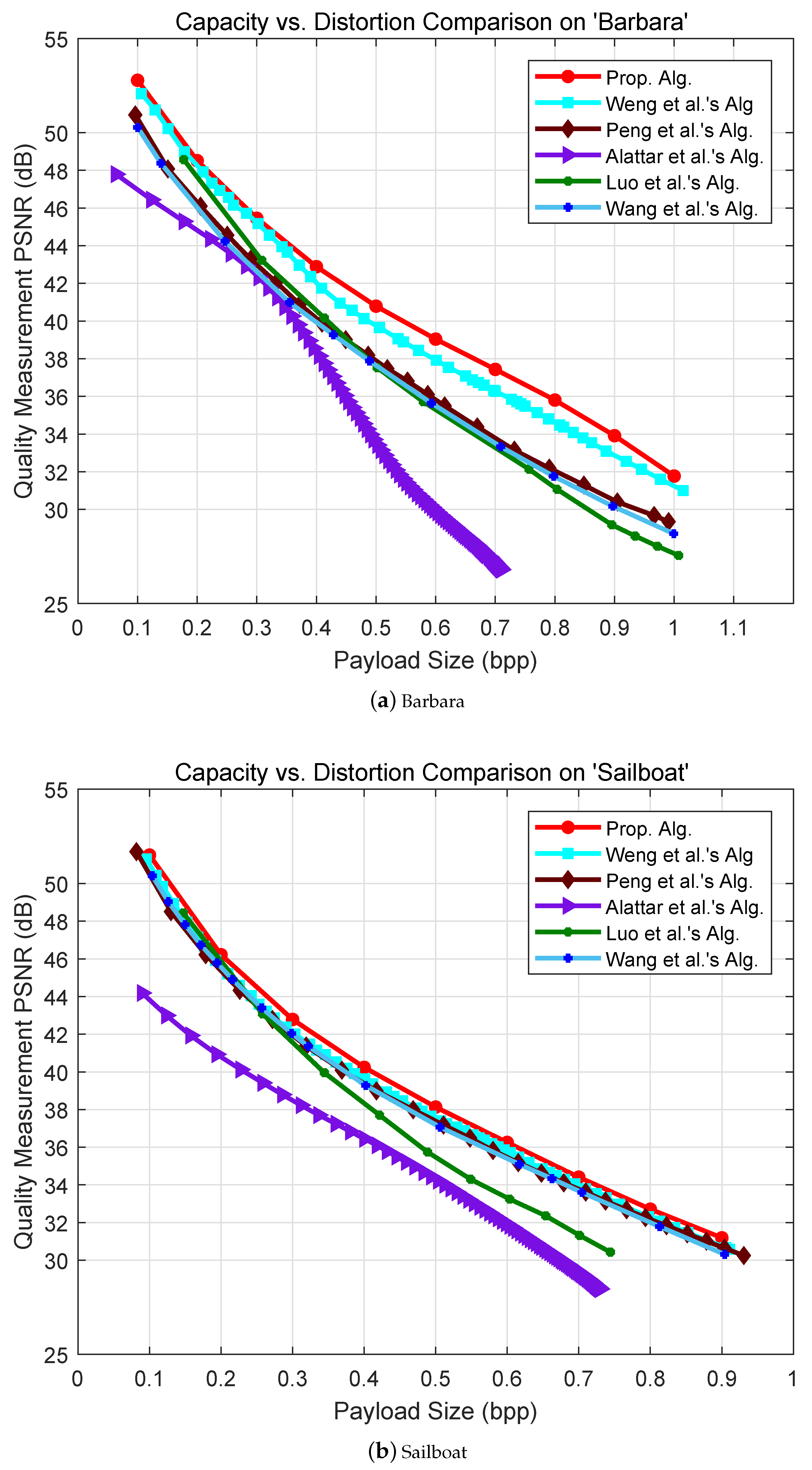
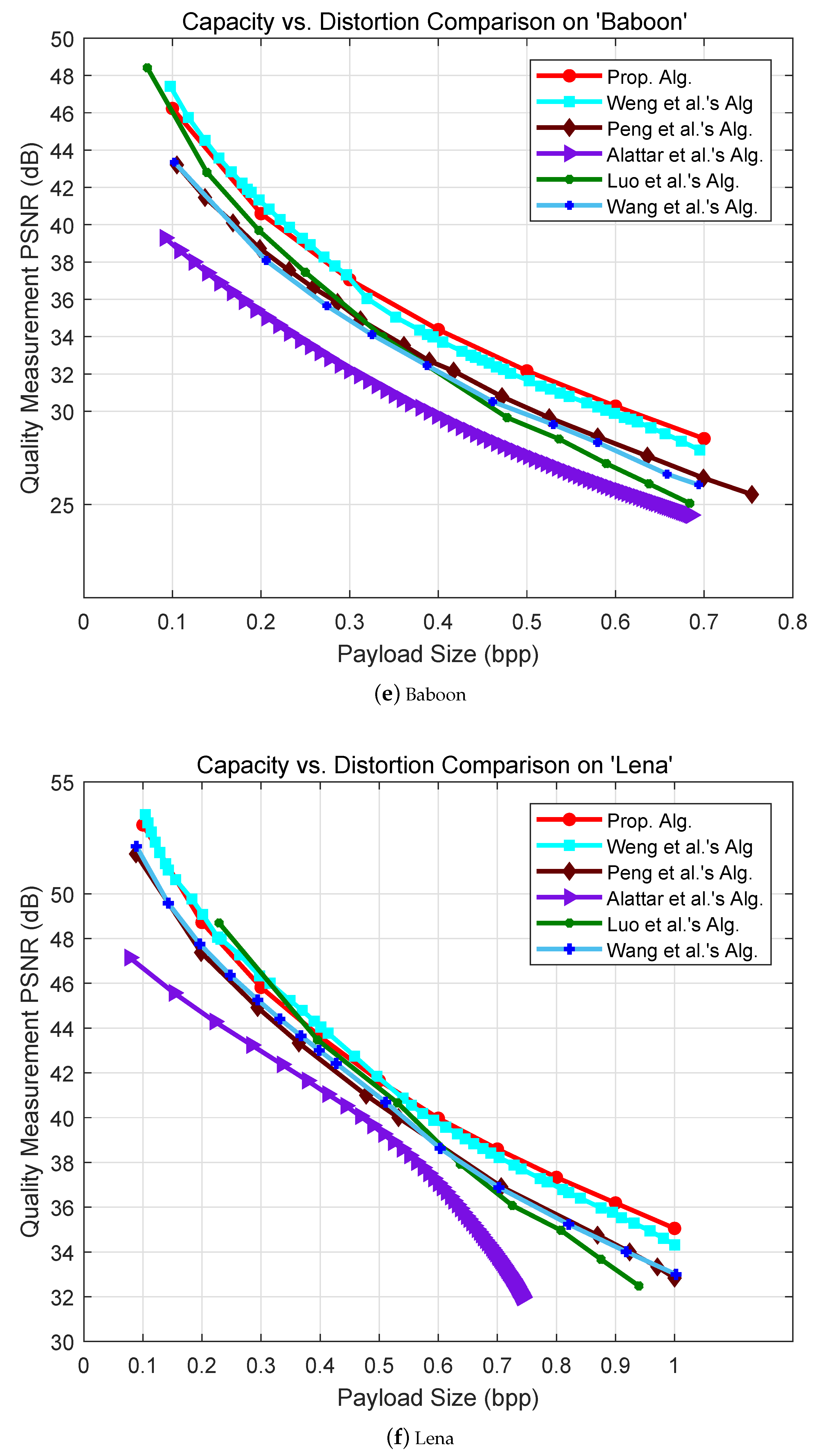
In the experiments, we compare our method with five RDH schemes proposed by Alattar [5], Wang et al. [6], Peng et al. [7], Weng et al. [8] and Luo et al. [16] so as to demonstrate our method is effective. Figure 5 illustrates comparisons of capacity-distortion performance among six RDH schemes on six images: Airplane, Baboon, Barbara, Goldhill, Sailboat and Lena.

Figure 5. Comparison of capacity-distortion performance among six reversible data hiding (RDH) schemes on six images: Airplane, Baboon, Barbara, Goldhill, Sailboat and Lena.

Our method achieves better performance compared with Alattar’s method by introducing block selection and irregular block partition. The experimental result also shows that the proposed method outperforms Alattar’s method. The integer transform proposed by Wang et al. can be thought to be a prediction process, in which the mean value of a block is used for predicting each pixel in this block. Their method is able to achieve high visual quality because there is not an additional term in Wang et al.’s scheme. However, when a block is used for data embedding, all the pixels must be expanded to carry data bits even if the distortion introduced by modified pixels is huge. In addition, it is very difficult to compress the location map which aims at differentiating the available blocks with unused ones in their method. In our method, the differences between every two pixels can be controlled by $p{T}_h$ so as to keep high visual quality. In the light of the invariant mean value, only the locations of the blocks identified to be within smooth regions are necessary to be recorded. To this end, in comparison to Wang et al.’s method, a location map with reduced size is required in our scheme and it is able to be remarkably compressed. In a word, our method achieves higher performance than Wang et al.’s. As an extension of Wang et al.’s method, Peng et al.’s method embeds more than one bit into each pixel in a block. Therefore, the problems in Wang et al.’s method are extended to Peng et al.’s. Thus, our method is superior to Peng et al.’s.

As for Airplane, Barbara, Goldhill and Sailboat in Figure 5, superior capacity-distortion performance can be obtained in our method at all embedding rates in contrast to Weng et al.’s. More specifically, slight increase in PSNR is introduced in our algorithm when low capacity is required, especially at the embedding rates smaller than 0.3 bpp. However, the proposed scheme provides significantly preferable performance at high embedding rates larger than 0.3 bpp. Experimental results in Baboon and Lena demonstrate that the distortion generated in our method is slightly higher than Weng et al.’s at low embedding rates. In contrast, when it comes to higher embedding rates (0.3 bpp for Baboon and 0.5 bpp for Lena), the performance is capable of exceeding that of Weng et al.’s method. In brief, the new algorithm is able to achieve more effective embedding performance, especially when larger embedding capacity is required. This is because the additional term provided in our method is smaller, which enables less distortion and better visual quality at the given embedding rates. Apart from small sized blocks, larger sized ones are also adopted in this paper. In this way, the embedding capacity increases dramatically while distortions produced by modification are low for the pixels located in smooth regions. In addition, unique prediction patterns employed in our method compensate for the shortage existing in large sized blocks i.e., weak intra-block correlation. In other words, more accurate prediction is achieved and a sharper difference histogram is formed.

6. Conclusions

In this paper, we propose a RDH method based on Alattar’s integer transform. The irregular block partition is adopted to increase the correlation between two pixels within a block. Since the mean value remains unchanged before and after data hiding, it is utilized to improve the prediction accuracy of block complexity. In addition, two-layer embedding is also introduced to enhance the embedding performance. The experimental results show that the proposed method achieves better embedding performance compared with prior state-of-the-art works.

References

- Celik, M.U.; Sharma, G.; Tekalp, A.M.; Saber, E. Lossless generalized-LSB data embedding. IEEE Trans. Image Process. 2005, 12, 157–160. [Google Scholar] [CrossRef]
- Tian, J. Reversible data embedding using a difference expansion. IEEE Trans. Circuits Syst. Video Technol. 2003, 13, 890–896. [Google Scholar] [CrossRef]
- Shi, Y.Q.; Ni, Z.C.; Zou, D.; Liang, C.Y.; Xuan, G.R. Lossless Data Hiding: Fundamentals, Algorithms and Applications. In Proceedings of the 2004 IEEE International Symposium on Circuits and Systems, Vancouver, BC, Canada, 23–26 May 2004; Volume 2, pp. 33–36. [Google Scholar]
- Thodi, M.; Rodriguez, J.J. Prediction-error based reversible watermarking. In Proceedings of the 2004 International Conference on Image Processing, Singapore, 24–27 October 2004; Volume 3, pp. 1549–1552. [Google Scholar]
- Alattar, A.M. Reversible watermark using the difference expansion of a generalized integer transform. IEEE Trans. Image Process. 2004, 13, 1147–1156. [Google Scholar] [CrossRef] [PubMed]
- Wang, X.; Li, X.L.; Yang, B.; Guo, Z.M. Efficient Generalized Integer Transform for Reversible Watermarking. IEEE Signal Process. Lett. 2010, 17, 567–570. [Google Scholar] [CrossRef]
- Peng, F.; Li, X.; Yang, B. Adaptive reversible data hiding scheme based on integer transform. Signal Process. 2012, 92, 54–62. [Google Scholar] [CrossRef]
- Weng, S.W.; Pan, J.S. Integer transform based reversible watermarking incorporating block selection. J. Vis. Commun. Image Represent. 2016, 35, 25–35. [Google Scholar] [CrossRef]
- Ni, Z.; Shi, Y.Q.; Ansari, N.; Su, W. Reversible data hiding. IEEE Trans. Circuits Syst. Video Technol. 2006, 16, 354–362. [Google Scholar]
- Li, X.L.; Li, B.; Yang, B.; Zeng, T.Y. General Framework to Histogram-Shifting-Based Reversible Data Hiding. IEEE Trans. Image Process. 2013, 22, 2181–2191. [Google Scholar] [CrossRef] [PubMed]
- Hu, Y.; Lee, H.K.; Li, J. DE-based reversible data hiding with improved overflow location map. IEEE Trans. Circuits Syst. Video Technol. 2009, 19, 250–260. [Google Scholar]
- Sachnev, V.; Kim, H.J.; Nam, J.; Suresh, S.; Shi, Y.Q. Reversible Watermarking Algorithm Using Sorting and Prediction. IEEE Trans. Circuits Syst. Video Technol. 2009, 19, 989–999. [Google Scholar] [CrossRef]
- Tsai, P.Y.; Hu, Y.C.; Yeh, H.L. Reversible image hiding scheme using predictive coding and histogram shifting. Signal Process. 2009, 89, 1129–1143. [Google Scholar] [CrossRef]
- Tai, W.L.; Yeh, C.M.; Chang, C.C. Reversible data hiding based on histogram modification of pixel differences. IEEE Trans. Circuits Syst. Video Technol. 2009, 19, 906–910. [Google Scholar]
- Hong, W.; Chen, T.S.; Shiu, C.W. Reversible data hiding for high quality images using modification of prediction errors. J. Syst. Softw. 2009, 82, 1833–1842. [Google Scholar] [CrossRef]
- Luo, L.; Chen, Z.; Chen, M.; Zeng, X.; Xiong, Z. Reversible image watermarking using interpolation technique. IEEE Trans. Inf. Forensic Secur. 2010, 5, 187–193. [Google Scholar]
- Hong, W. An efficient prediction-and-shifting embedding technique for high quality reversible data hiding. EURASIP J. Adv. Signal Process. 2010, 2010. [Google Scholar] [CrossRef]
- Coltuc, D. Improved embedding for prediction-based reversible watermarking. IEEE Trans. Inf. Forensic Secur. 2011, 6, 873–882. [Google Scholar] [CrossRef]
- Gao, X.; An, L.; Yuan, Y.; Tao, D.; Li, X. Lossless data embedding using eneralized statistical quantity histogram. IEEE Trans. Circuits Syst. Video Technol. 2011, 21, 1061–1070. [Google Scholar]
- Li, X.L.; Yang, B.; Zeng, T.Y. Efficient Reversible Watermarking Based on Adaptive Prediction-ErrorExpansion and Pixel Selection. IEEE Trans. Image Process. 2011, 20, 3524–3533. [Google Scholar]
- Wu, H.T.; Huang, J.W. Reversible image watermarking on prediction errors by efficient histogram modification. Signal Process. 2012, 92, 3000–3009. [Google Scholar] [CrossRef]
- Coatrieux, G.; Pan, W.; Cuppens-Boulahia, N.; Cuppens, F.; Roux, C. Reversible watermarking based on invariant image classification and dynamic histogram shifting. IEEE Trans. Inf. Forensic Secur. 2013, 8, 111–120. [Google Scholar] [CrossRef]
- Jung, S.; Ha, L.; Ko, S. A new histogram modification based reversible data hiding algorithm considering the human visual system. IEEE Signal Process. Lett. 2011, 18, 95–98. [Google Scholar] [CrossRef]
- Hong, W.; Chen, T.; Wu, M. An improved human visual system based reversible data hiding method using adaptive histogram modification. Opt. Commun. 2013, 291, 87–97. [Google Scholar] [CrossRef]
- Weng, S.W.; Pan, J.S. Reversible watermarking based on multiple predictionmodes and adaptive watermark embedding. Multimed. Tools Appl. 2013, 72, 3063–3083. [Google Scholar] [CrossRef]
Figure 1.
Taking a -sized block for example, a two-dimensional image block is arranged into a one-dimensional pixel list according to the arrow direction.
Figure 2.
Various-sized image blocks.
Figure 3.
An -sized block is marked in black, and its neighborhood is composed of pixels marked in green, where .
Figure 4.
Four modes.
Figure 5.
Comparison of capacity-distortion performance among six reversible data hiding (RDH) schemes on six images: Airplane, Baboon, Barbara, Goldhill, Sailboat and Lena.