Exploration with Multiple Random ε-Buffers in Off-Policy Deep Reinforcement Learning

Abstract

In terms of deep reinforcement learning (RL), exploration is highly significant in achieving better generalization. In benchmark studies, ε-greedy random actions have been used to encourage exploration and prevent over-fitting, thereby improving generalization. Deep RL with random ε-greedy policies, such as deep Q-networks (DQNs), can demonstrate efficient exploration behavior. A random ε-greedy policy exploits additional replay buffers in an environment of sparse and binary rewards, such as in the real-time online detection of network securities by verifying whether the network is “normal or anomalous.” Prior studies have illustrated that a prioritized replay memory attributed to a complex temporal difference error provides superior theoretical results. However, another implementation illustrated that in certain environments, the prioritized replay memory is not superior to the randomly-selected buffers of random ε-greedy policy. Moreover, a key challenge of hindsight experience replay inspires our objective by using additional buffers corresponding to each different goal. Therefore, we attempt to exploit multiple random ε-greedy buffers to enhance explorations for a more near-perfect generalization with one original goal in off-policy RL. We demonstrate the benefit of off-policy learning from our method through an experimental comparison of DQN and a deep deterministic policy gradient in terms of discrete action, as well as continuous control for complete symmetric environments.

1. Introduction

Deep reinforcement learning (RL) [1] has been applied in challenging domains, such as games and robotics. A combination of RL and nonlinear function approximates, such as deep neural networks, helps in automating decision making and control issues. However, it can also be challenging in terms of stability and convergence [2] in real-time online learning, such as in the detection of network security through the verification of whether the network is “normal or anomalous” [3,4,5,6,7]. Moreover, its widespread adaptation in the real world, such as with robotic arms, is difficult because of sample complexity and heavy dependence on certain hyper-parameters, such as exploration constants [3,4,5,6,7]. A significant challenge in robotics is the engineering of a carefully shaped reward function. However, the necessity of reward function engineering restricts the general applicability of RL in the real world. Recent remarkable research on hindsight experience replay (HER) [8] provides additional replay buffers with the original goal and a subset of other goals without any domain knowledge. HER improves the sample-efficient setting and learns the possible multi-goals, even in an environment of sparse rewards. Off-policy algorithms in RL [1], such as deep Q-networks (DQNs) [9,10], reuse the past experience with random ε-greedy actions in replay buffers for efficient exploration behaviors. Andrychowicz et al. [8] found that a DQN combined with HER resolves some tasks more easily than that without HER. An experience comprises a tuple, such as state, action, reward, or new state, and each agent of DQN can exploit a batch of experiences to update the Q-value function via temporal differencing (TD) learning [9,10]. The experience replay (ER) buffer discards old memories at each step by sampling the buffer randomly and updating the DQN agent. It aids in breaking temporal relations and increasing data usage [11,12].

The present study is inspired by the quantification of generalization in RL [11], which investigates the impact of injecting stochastic methods on generalization by random ε-greedy actions overriding the agent’s preferred actions. A random ε-greedy action has been used to encourage exploration and prevent excessive over-fitting [11]. There has been research on the exploration diversities of stability and convergence. A prioritized replay memory [13] has been used in a DQN for replaying important transitions more frequently and learning more efficiently. HER [8] makes possible sample-efficient learning with additional replay buffers. A parameter space in noise [14] in a neural network leads to a more abundant set of exploratory behaviors through noise injection in the action space in deep RL. However, some empirical implementations show that in certain environments, adding parameter space noise [14] may not improve ε-greedy random actions by OpenReivew.net [15]. A prioritized replay memory attributed to a complex TD error might provide better theoretical results. The TD errors might create a balance issue between variance and bias, because TD attributes can be computed at every n-time step [11,12]. Moreover, some studies have only partially succeeded in combining drop-out, L2 regularization, and ε-greedy random actions. Thus, training with only ε-greedy random actions can vastly improve generalization and exploration [11,12].

This paper proposes multiple ε-greedy experience buffers in off-policy deep RL [1] for enhancing explorations for a more near-perfect generalization for the original goal. We consider strengthening the advantages of exploring model-free, deep RL, and demonstrate that the off-policy method benefits through the experimental comparison of DQN [9,10] and DDPG [16], which is actually based on on-policy, and represents a trade-off between policy optimization [2,16] and Q-learning [9,10]. The proposed deep RL model is compatible with the discrete action as well as continuous control, symmetrically. Therefore, we can expect better prediction accuracy in real-time online learning, such as detecting network intrusions by verifying whether the network is “normal or anomalous” [3,4,5,6,7]. The concept of our proposed multiple ε-buffers is extremely simple. After experiencing some episodes, we store them in the replay buffers R₁ and R₂. Note that we can replay one trajectory with only one goal, assuming that we exploit an off-policy RL like DQN [9,10] and DDPG [16]. When the procedure passes through multiple ε-buffers, the trade-off between policy optimization and Q-learning can be solid and strong due to the deep neural network in DQN [9,10] or DDPG [16].

2. Background

RL comprises an agent with an environment that is described by a set of states, S, a set of actions, A, a distribution of initial states, p(s₀), a reward function, r: S × A → R, transition probabilities, p(s_t+1|s_t,a_t), and a discount factor, γ ∈ [0,1] [1]. Deterministic policy maps from states to actions are given as π: S → A. At each time step, t, the agent selects an action attributed to the current state: a_t = π(s_t), and takes the reward, r_t = r(s_t,a_t) [1]. The new state of the environment is sampled from the distribution p(|s_t,a_t). A discounted cumulative reward is a return, R_t = ∑Tγ^t’−tr_t’, where T is the time step at which the agent’s simulation terminates [1]. The goal here is to maximize its expected return E_s0[R₀|s₀]. The action value function, named Q-function, is defined as Q^π(s_t,a_t) = E[R_t|s_t,a_t]. An optimal policy is denoted by the following equation, called the Bellman equation, Q*(s,a) = E_s’~p(|s,a) [r + γmax_a’Q*(s’,a’)|s,a], (1), this equation converges at the Q-function as an optimal action value [1]. The Bellman equation is to be used as a function approximation for estimating the Q-function, Q(s,a;θ) ≈ Q*(s,a), as an action value [1]. This can be a linear-function approximation, but it is sometimes even a nonlinear-function approximation, such as with a deep neural network [9,10]. Therefore, we attempt to exploit a deep neural network as a function approximation. We refer to a deep neural network approximation with weights θ as the Q-function [9,10]. A Q-function network can be trained by minimizing a sequence of loss functions, L_i(θ_i), which changes at i per iteration [1,9,10]. L_i(θ_i) = E_s,a~p(|s,a)[(y_i − Q(s,a;θ_i))²], (2), where y_i = E_{s’∼p(|s,a)} [r + γmax_a’Q*(s’,a’;θ_i−1)|s,a] is the target for i per iteration. The loss function can be differentiated with regard to the weights, depending on the gradient [1,9,10]. ∇θ_iL_i(θ_i) = E_{s,a~p(|s,a);s’~ε}[r + γmax_a’Q(s’,a’;θ_i−1) − Q(s,a;θ_i))∇θ_iQ(s,a;θ_i)], (3), [1,9,10]. Optimizing the loss function by using the stochastic gradient descent is computationally intricate. Q-learning as a function approximation becomes possible [17,18], and is model-free, which indicates the RL model and off-policy. This implies that it learns about greedy strategy a = max_aQ(s,a;θ) while obeying an exploration selected by ε-greedy with a probability of 1 − ε and a random action with a probability of ε for exploration and exploitation [17,18]. DQN is a well-known, model-free RL algorithm attributed to discrete action spaces. In DQN [9,10], we construct a deep neural network, Q, which approximates Q^∗ and is greedy-defined as π_Q(s) = argmax_a∈AQ(s,a) [9,10]. It is a ε-greedy policy with probability ε and takes the action π_Q(s) with probability 1 − ε. Each episode uses the ε-greedy policy following Q as an approximation of the deep neural network. The tuples (s_t, a_t, r_t, s_t+1) are stored in the replay buffer, and each new episode is configured to neural network training [9,10]. The deep neural network is trained using the gradient descent of random episodes on loss L, encouraging Q to follow the Bellman equation [9,10]. The tuples are sampled from the replay buffer of random episodes. The target network y_t is computed by a separate neural network that changes more slowly than the main deep neural network in order to optimize a stable process. The weights of the target network are set to the current weights of the main deep neural network. The DQN algorithm [9,10] is presented in Algorithm 1.

Algorithm 1 Deep Q-learning with Experience Replay

Initialize replay memory D to capacity N Initialize action-value function Q with random weights for episode = 1, M do   Initialize sequence s1 = {x1} and preprocessed sequenced ϕ1 = ϕ (s1)   for t = 1, T do     With probability ε, select a random action αt     Otherwise select αt = maxαQ*(ϕ(st),α;θ)     Execute action αt in emulator and observe reward rt and image xt+1     Set st+1 = st, αt, xt+1 and preprocess ϕt+1 = ϕ(st+1)     Store transition (ϕt, αt, rt, ϕt+1) in D     Sample random mini-batch of transitions (ϕj, αj, rj, ϕj+1) from D     Set  yj = rj            for terminal ϕj+1     Or  yj = rj + γmaxα’Q *(ϕj+1,α’;θ)  for non-terminal ϕj+1     Perform a gradient descent step on (yj − Q(ϕj, αj |θ))2   end for end for

A deep deterministic policy gradient (DDPG) [16] is a well-known, model-free RL algorithm attributed to continuous action spaces [2,16]. In a DDPG, we construct two neural networks: a target policy as an actor, π: S → A, and an action-value-function approximation as a critic, Q: S × A → R. The critic approximates Q^π, which is the action-value function of the actor [16]. Each episode uses a noisy policy of the target, π_b(s) = π(s) + Ɲ(0,1) [16]. The critic is trained in the same way as the Q-function in a DQN [9,10]. The target network yt is computed using the output of the actor, i.e., y_t = r_t + γQ(s_t+1, π(s_t+1)), and the actor’s deep neural network is trained using the gradient descent of random episodes on the loss L_a = −E_sQ(s,π(s)) [2,16] and sampled from the replay buffer of random episodes. The gradient of L_a is computed by both the critic and actor through back-propagation [2,16]. The algorithm of a DDPG [16] is shown in Algorithm 2.

Algorithm 2 Deep Deterministic Policy Gradient

Randomly initialize critic Q(s, a|θQ) and actor μ(s|θμ) with weights θQ and θμ Initialize target Q’ and μ’ with weights θQ’← θQ, θμ’ ← θμ Initialize replay memory R for episode = 1, M do   Initialize a random process N for action exploration   Receive initial observation state s1   for t = 1, T do     Select action αt = μ(st|θμ) + Ɲt according to the current policy and exploration noise     Execute action αt and observe reward rt and new state st+1     Store transition (st, αt, rt, st+1) in R     Sample random mini-batch of transitions (sj, αj, rj, sj+1) from R     Set yj = rj + γQ’(sj+1, μ’(sj+1|θμ’)|θQ’)     Update critic by minimizing the loss: L = $\frac{1}{\mathrm{n}}{\Sigma }_{\mathrm{j}}$(yj − Q(sj, αj|θQ))2     Update the actor policy using the sampled policy gradient:       ∇θμI≈ $\frac{1}{\mathrm{n}}{\Sigma }_{\mathrm{j}}$∇αQ(s,α|θQ)|s = sj, α = α μ(sj)∇θμμ(s|θμ)|sj     Update the target:        θQ’← τθQ+(1−τ) θQ’        θμ’← τθμ+(1−τ) θμ’   end for end for

3. Multiple Random ε-Buffers

3.1. Proposed Off-Policy Algorithm

We propose multiple random ε-greedy buffers in a DQN [9,10] for discrete action spaces and DDPG [2,16] for continuous action spaces. The idea of our proposed multiple ε-buffers is to store experienced episodes in the replay buffers R₁ and R₂. For better exploration, the agent evaluates a target policy π(a|s) to compute Vπ (s) or Qπ(s,a) while following a behavior policy μ(a|s), where {s₁, a₁, r₂, … s_T} ~ μ. The agent learns about multiple policies while following one policy. This means that it can learn about the optimal policy and follow the exploratory policy. The target policy π is greedy with respect to Q(s,a), such as π(s_t+1) = argmax_a’Q(s_t+1,a’), while the behavior policy μ is ε-greedy with respect to Q(s,a), such as μ(s_t+1) = R_t+1 + max_a’γQ(s_t+1,a’). When an agent follows a greedy policy, convergence changes rapidly. However, because of a lack of exploration, the agent reaches local optimization. Many other challenges address this global–local dilemma [2,9,10,16]. A remarkable recent work, HER [8], provides additional replay buffers with the original goal and a subset of other goals without any complicated reward function. The off-policy algorithms in RL, such as DQN [9,10] or DDPG [2,16], reuse the past experience with random ε-greedy actions in replay buffers for better exploration. The ER buffers discard old memories at each step by sampling the buffer randomly to update the DQN agent. Therefore, ER helps to break temporal relations and increase data usage [11,12].

Our study is inspired by quantifying generalization in RL [11], which provides a random ε-greedy action that has been used to encourage exploration and prevent excessive over-fitting. A prioritized replay memory [13] has been exploited in a DQN to replay important transitions. A parameter space in the noise [14] of a neural network leads to a more abundant set of exploratory behaviors. These recent studies have shown how HER [8] can improve random ε-greedy actions. Therefore, we consider enhancing multiple random ε-greedy experience buffers in deep RL for more near-perfect explorations for the original goal. We demonstrate the off-policy learning benefit from our method through an experimental comparison of DQN [9,10] and DDPG [2,16] in high-dimensional discrete action environments as well as continuous control tasks. Our idea is that after experiencing some episodes, we store them in the replay buffers R₁ and R₂. We can replay one trajectory with only one goal, assuming that we exploit an off-policy RL like DQN [9,10] and DDPG [2,16]. While the procedure passes through multiple random ε-buffers, the balance between variance and bias of the policy can be solid and strong due to the training of the deep neural network.

Without using a complicated shaping reward and knowledge environment, we attempt to achieve a near-perfect global optimal goal. This idea is also used in the HER [8] and ODE model [12]. We attempt to achieve better exploration, which can balance computational speed and global optimization. If we use both a target policy and an alternative policy, we can attain the previously achieved global optimization. Subsequently, we consider the computational speed while maintaining generalization. HER [8] stores each transition in the replay buffer not only with the original goal, but also with a subset of other goals. However, we increase the number of replay buffers, which are a minimum of two. Therefore, we can replay each trajectory with two or more buffers, assuming that we use an off-policy RL algorithm, such as DQN [9,10] or DDPG [2,16], for a complete symmetric environment. Similar to HER [8], our proposed model can learn with extremely sparse rewards, and performs better in our experiments. These results indicate the practical challenges with reward shaping, such as HER [8]. Moreover, we can acquire the results of the effects of memory size from ODEs [12]. The selection of memory size does not have any effect on learning behavior; there is a trade-off between an over-fitting and the weight update [12]. If the memory size is smaller, the process of learning is probably over-fitted. Similarly, if the memory is bigger, the over-fitting effect is alleviated. However, it is not easy to deal with the balance between over-fitting and weight update [11,12]. With prioritized replay [13], if the memory size is small, especially if the mini-batch is small, then the trade-off between the over-fitting and weight update is more consequential. Therefore, we consider enhancing the characteristic feature of model-free RL, i.e., increasing the number of random ε-buffers. In terms of policy optimization, the policy πθ(s,a) is explicit, and for performance optimization, the agent follows the policy πθ(s,a) directly. Therefore, we call it on-policy optimization. However, Q-learning is based on off-policy, because it can learn about an optimal policy with respect to Q(s,a), such as π(s_t+1) = argmax_a’Q(s_t+1,a’), and follow an exploratory policy [1]. Policy optimization [2,16] is more stable than Q-learning [9,10]; however, Q-learning [9,10] is more sample-efficient than policy optimization [2,16]. Therefore, we follow the lead to strengthen the advances in model-free RL. DDPG [16] is actually based on on-policy [1]. However, it can create a good trade-off between policy optimization [2,16] and Q-learning [9,10]. Algorithms 3 and 4 display the DQN and DDPG algorithm, respectively, with multiple random ε-buffers.

Algorithm 3 Deep Q-learning with multiple random ε-buffers

Initialize replay memory R1 and R2 Initialize Q-function with random weights for episode = 1, M do   Initialize sequence s1 and ϕ1 = ϕ (s1)   for t = 1, T do     With probability ε, select a random action αt       Or select αt = maxαQ *((st), α;θ)     Execute action αt in emulator and observe reward rt     Set st+1 = st, αt and ϕt+1 = ϕ (st+1)      Store transition (ϕt, αt, rt, ϕt+1) in R1         //standard experience buffer      Store transition (ϕt, αt, rt, ϕt+1) in R2         //second experience buffer     Sample random mini-batch of transitions (ϕj, αj, rj, ϕj+1) from either R1 or R2      Set yj = rj         Or yj = rj + γmaxα’Q*(ϕj+1, α’|θ)     Perform a gradient descent step on (yj − Q(ϕj, αj|θ))2   end for     Sample random mini-batch of transitions from either R1 or R2 end for

3.2. Algorithm Description

3.2.1. DQN with Multiple Random ε-Buffers

• Initialize replay memories of both R₁ and R₂ and Q(s,a), and initiate the process from a random state, s.
• Initialize the sequence with the start state, s.
• The agent learns the policy max_αQ*((s_t,a);θ) with greed and follows another policy with probability ε.
• For exploration, an experience composed of a tuple, such as (state s, action a, reward r, new state s’), is in both R₁ and R₂.
• Sample a random mini-batch of transitions from either R₁ or R₂.
• The weights for performing the gradient descent (r_j + γmax_α’Q*(ϕ_j+1, α’|) − Q(ϕ_j, α_j|θ)) for a target DQN with multiple random ε-buffers.
• Steps 3–6 are repeated for training.
• For the next episode, sample a random mini-batch of transitions from either R₁ or R₂.
• Steps 2–8 are repeated for training.

3.2.2. DDPG with Multiple Random ε-Buffers

• Initialize critic deep network Q(s, a|θ^Q) and actor deep network μ(s|θ^μ).
• Initialize replay memories in both R₁ and R_2.
• The agent selects the action according to the current policy, α_t = μ(s_t|θ^μ) + Ɲ_t.
• For exploration, an experience composed of a tuple, such as (state s, action a, reward r, new state s’), is in both R₁ and R₂.
• A mini-batch of transitions is randomly sampled from either R₁ or R₂.
• The critic network is updated by the loss function L = 1/n∑_j(r_j + γQ’(s_j+1, μ’(s_j+1|θ^μ’)|θ^Q’) − Q(s_j, α_j |θ^Q))².
• The actor network is updated by the policy gradient descent ∇θμI ≈ 1/n∑_j∇_αQ(s|θ^Q)|s = s_j, α = α μ(s_j) ∇_θμμ(s|θ^μ)|s_j for a target DDPG with multiple random ε-buffers.
• Update the target network θ^Q’ ← τθ^Q + (1 − τ) θ^Q’ and θ^μ’ ← τθ^μ + (1 − τ) θ^μ’.
• Steps 3–8 are repeated for training.
• For the next episode, a mini-batch of transitions is randomly sampled from either R₁ or R₂.
• Steps 2–10 are repeated for training.

Algorithm 4 Deep Deterministic Policy Gradient with multiple random ε-buffers

Initialize critic Q(s, a|θQ) and actor μ(s|θμ) with weights θQ and θμ Initialize target Q’ and μ’ with weights θQ’← θQ, θμ’ ← θμ Initialize replay memory R1 and R2 for episode = 1, M do   Initialize observation s1 and a random process N for action exploration   for t = 1, T do     Select action αt = μ(st|θμ) + Ɲt by the current policy and exploration noise     Execute action αt and observe reward rt and new state st+1       Store transition (st, αt, rt, st+1) in R1          //standard experience buffer       Store transition (st, αt, rt, st+1) in R2          //second experience buffer     Sample a random mini-batch of transitions (sj, αj, rj, sj+1) from either R1 or R2       Set yj = rj + γQ’(sj+1, μ’(sj+1|θμ’)|θ Q’)       Update critic by minimizing the loss: L = $\frac{1}{\mathrm{n}}{\Sigma }_{\mathrm{j}}$(yj − Q(sj, αj|θQ))2     Update the actor by the sampled policy gradient:         ∇θμI≈ $\frac{1}{\mathrm{n}}{\Sigma }_{\mathrm{j}}$∇αQ(s,α|θQ)|s = sj, α = α μ(sj)∇θμμ(s|θμ)|sj       Update the target:         θ Q’← τθQ+(1−τ) θ Q’          θ μ’← τθμ+(1−τ) θ μ’   end for     Sample a random mini-batch of transitions from either R1 or R2 end for

4. Evaluation and Results

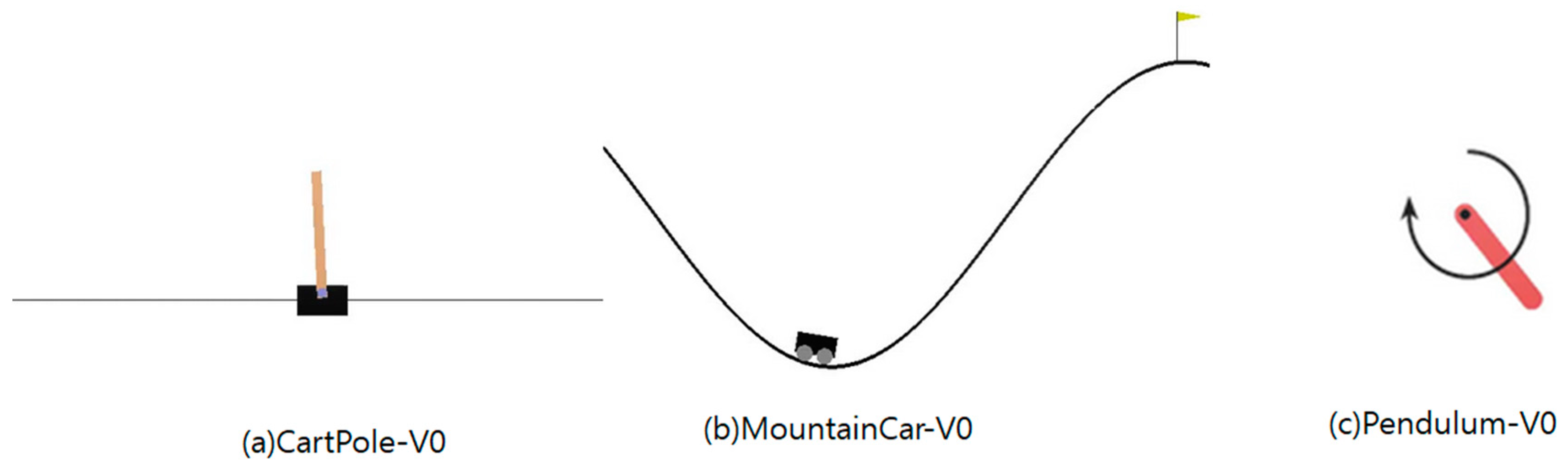
We consider OpenAI Gym [19] for our proposed algorithms, i.e., DQN and DDPG with multiple random ε-buffers. To enhance multiple random ε-greedy experience buffers, we exploit classic control environments in OpenAI Gym, such as CartPole-v0 [20,21], MountainCar-v0 [22,23], and Pendulum-v0 [24,25]. With similar approaches [9,10], we exploit a method, known as experience replay. Moreover, in our proposed method, Q-learning stores past experiences at each time step, e_t = (s_t, a_t, r_t, s_t+1), in multiple random ε-buffers, R₁ and R₂. Our emulators from OpenAI Gym [19] can apply mini-batch updates into R₁ and R₂. After the multiple random experience replay memories, the agent’s actions of the emulator follow ε-greedy policy. In terms of DQN with multiple random ε-buffers, for enhanced exploration, we also follow the theory of the target Q-network of breakthrough research in [9,10]. The Q-learning agent calculates the TD error with the current estimated Q-value [9,10]. The optimized action-value function follows a significant identity, known as the Bellman equation [9,10]. In accordance with this equation, the TD target is the reward based on an action in the state plus the discounted highest Q-value for the next state [9,10]. In terms of DDPG with multiple random ε-buffers, for enhanced exploration, we also follow the theory of the critic and actor networks in [2,16]. Because the Q-learning of DDPG can exploit the deterministic policy, argmax_aQ, our proposed method can follow the off-policy [1].

For DQN with multiple random ε-buffers, we exploit CartPole-V0 [20,21] and MountainCar-V0 [22,23]. In CartPole-V0 [20,21], a pole is attached with an unactuated joint to a cart moving along a frictionless track. It is controlled by forcing +1 or −1 to the cart. The pole starts upright, and the goal is to prevent it from falling over. A + 1 reward is given to every time step in which the pole remains upright. The episode stops when the pole is more than 15° from the vertical direction or the cart moves more than 2.4 units from the center. In our simulation, CartPole-V0 defines “solving” as if the average reward is more than 490 or equal to 500 over 10 consecutive runs. The agent of CartPole-V0 receives −100 reward if it falls over prior to the max-length of the episode [21]. In MountainCar-V0, a car is on a one-dimensional track, positioned between two mountains, with the goal of driving up the mountain on the right. The engine of the car is not strong enough to scale the mountain in a single pass. Therefore, the only way to succeed is to drive back-and-forth to reach the other side of the mountain. MountainCar-V0 defines “solving” as obtaining an average reward of −110 over 100 consecutive trails [23]. In Pendulum-V0, the inverted pendulum starts from a random position, and the goal is to swing it upwards so that it stays upright. Pendulum-V0 is an unsolved environment, which means that it does not have a special reward threshold at which it is considered solved [24,25].

Our proposed DQN and DDPG with multiple random ε-buffers were implemented using TensorFlow [26] and Keras [27] in OpenAI Gym [19].

4.1. CartPole-V0

For DQN with multiple random ε-buffers, we follow similar previous studies [21]. In Figure 1a, there is a CartPole-V0 [20] by OpenAI Gym [19]. Thus, GAMMA = 0.95, LEARNING − RATE = 0.001, MEMORY − SIZE = 10,000, BATCH − SIZE = 64, EXPLORATION − MAXIMUM = 1.0, EXPLORATION − MININUM = 0.01, and EXPLORATION − DECAY = 0.995 are the same as with the previous DQN studies [21] because of a fairness comparison.

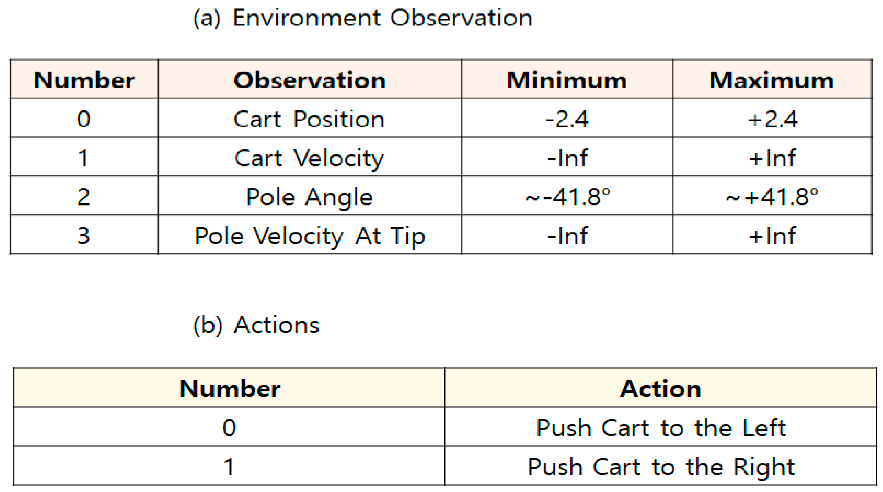
In the Cart-Pole-V0 environment, there are four observations and two discrete actions; see Figure 2. Furthermore, there are three episode terminations: the pole angle is more than −12° or + 12°, the cart position is more than −2.4 or + 2.4, and the episode length is greater than 200 [20].

However, the requirements from the implementation research can be considered in order to obtain better solutions [21]. Q-learning receives −100 as the reward when it falls before the maximum length of the episode is reached. Moreover, if the average reward is more than 490 or equal to 500 over 10 consecutive runs, Q-learning is terminated, even before it attains the maximum length of the episode [21].

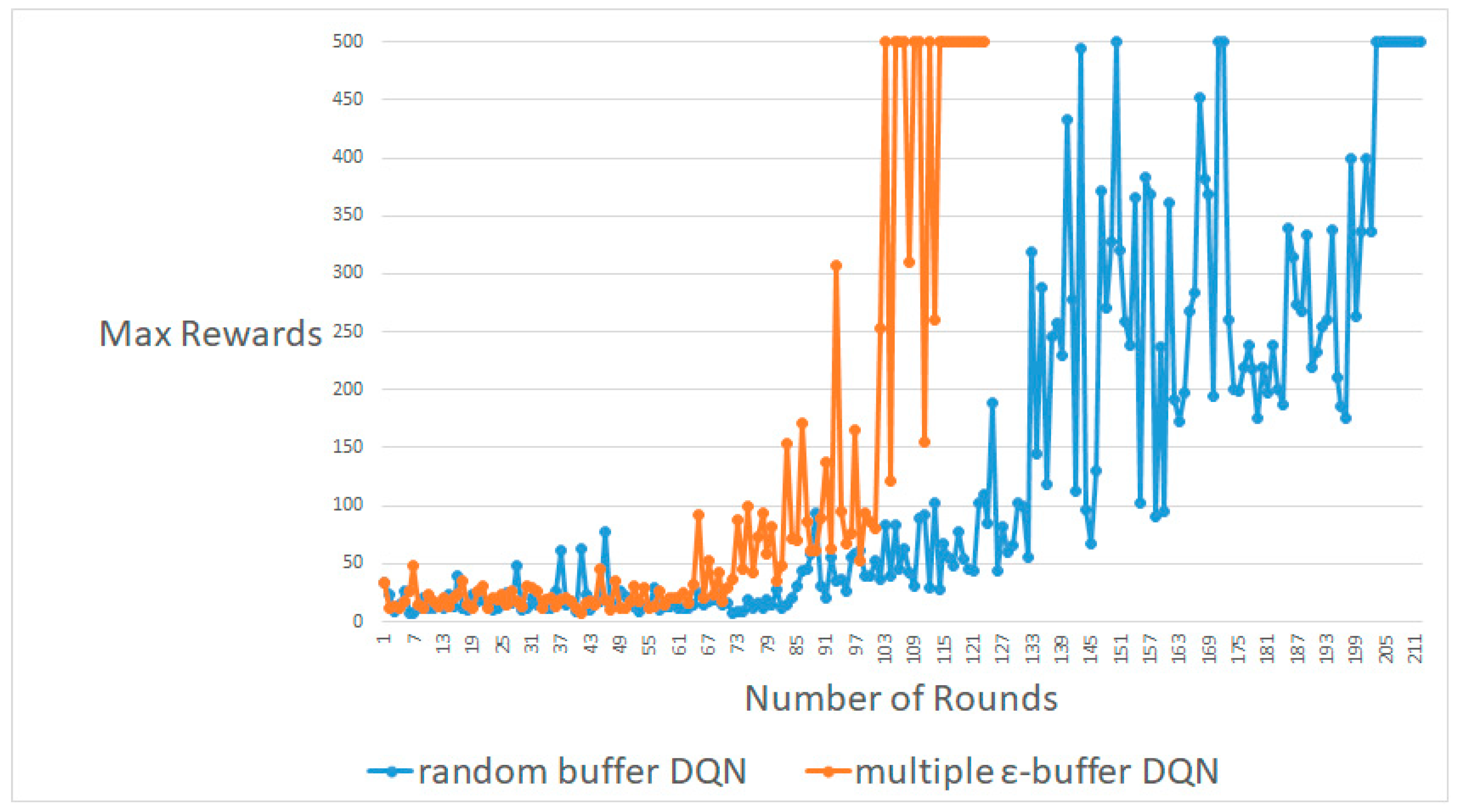
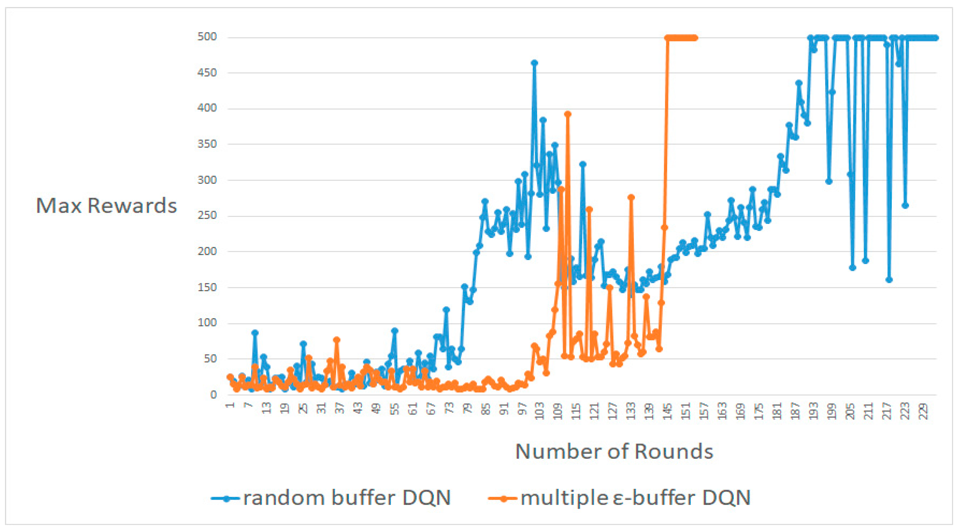
Figure 3, Figure 4 and Figure 5 display most of the results for the average, worst, and best cases, respectively. A DQN with multiple random ε-buffers can yield better results than one random buffer. In each of the average, worst, and best cases, our proposed method reaches the maximum reward earlier than DQN with one random buffer. Therefore, we can simulate identical results in real-time online for information security in Big Data. If our proposed method is used in training in real-time online in deep RL, as in a recent study [3,4,5,6,7], we acquire better results. Moreover, we can attempt a different deep neural network and hyper-parameter settings to demonstrate that our proposed model can enhance the exploration without specific domain information. We are convinced that we can enhance the behavior policy. Therefore, our proposed method can advance the exploration performance of ε-greedy, because multiple mini-batches do not follow a local minimum [9,10].

4.2. MountainCar-V0

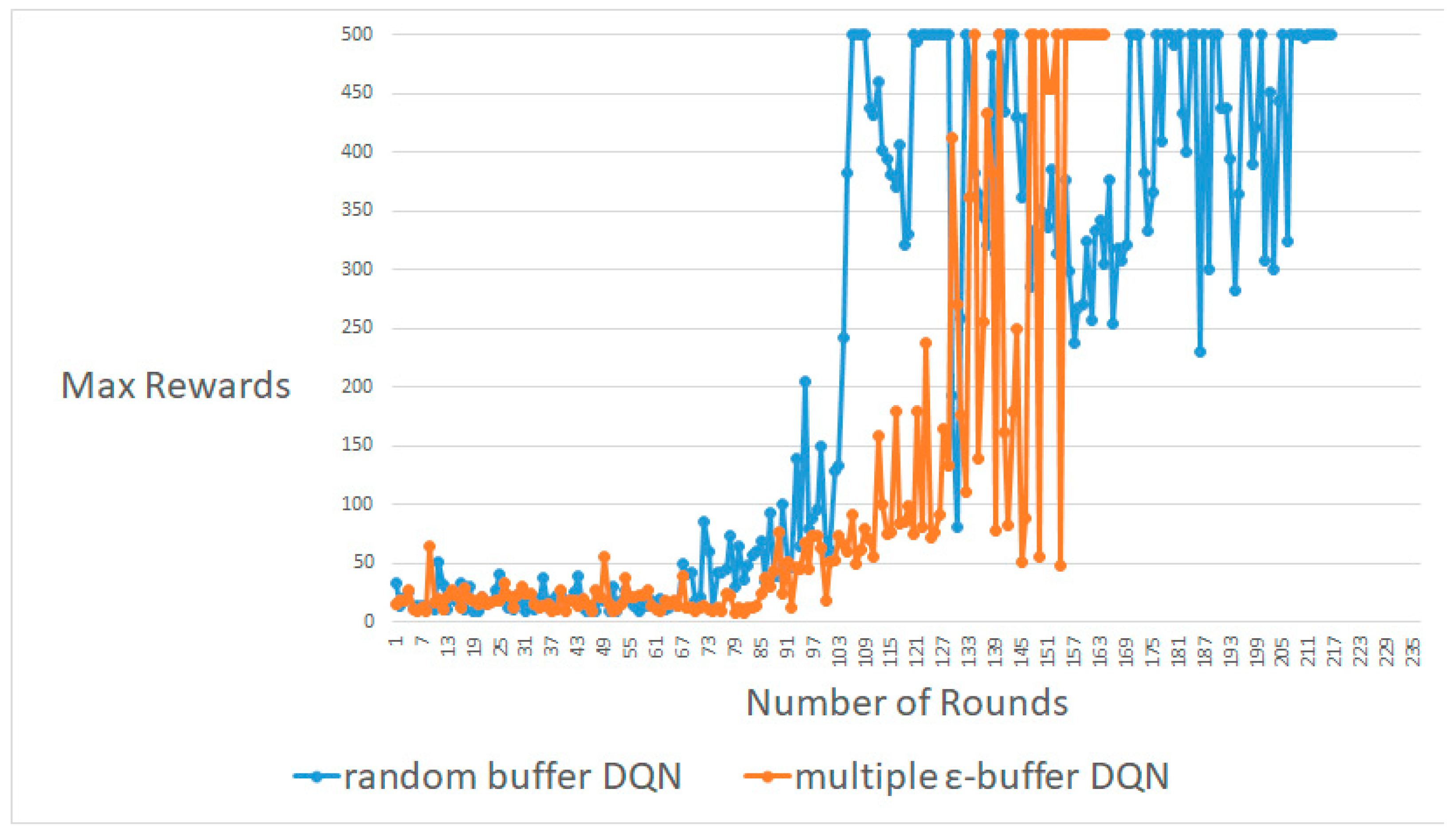
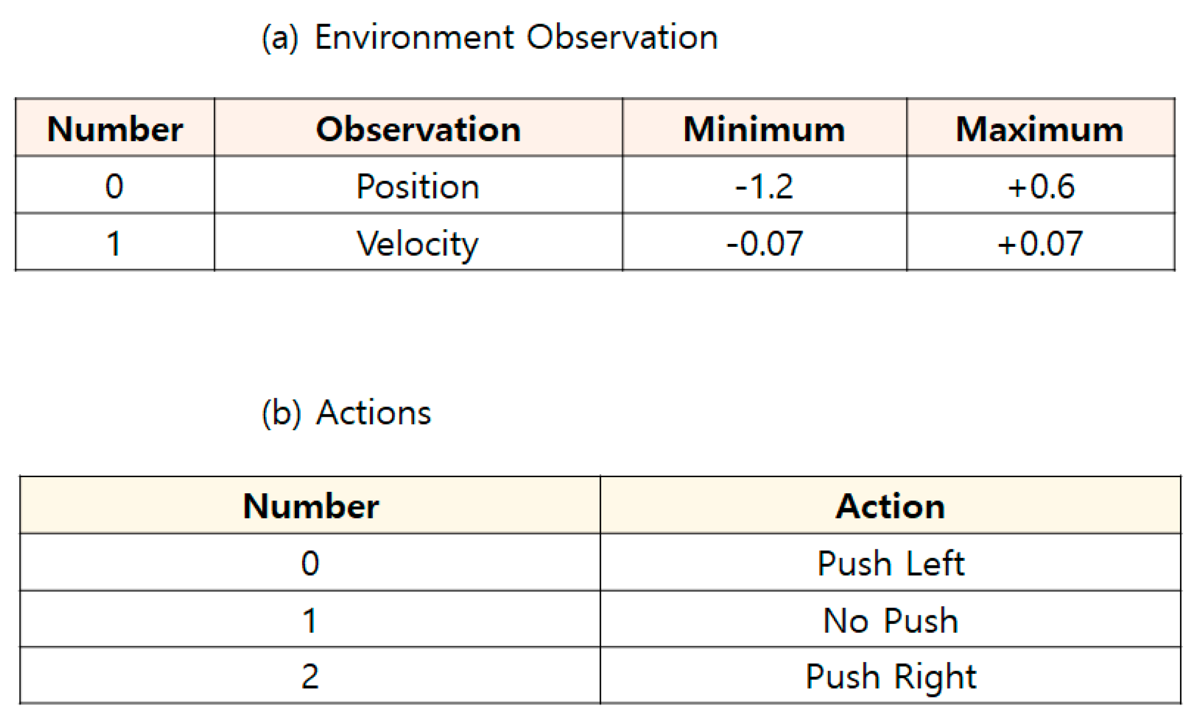
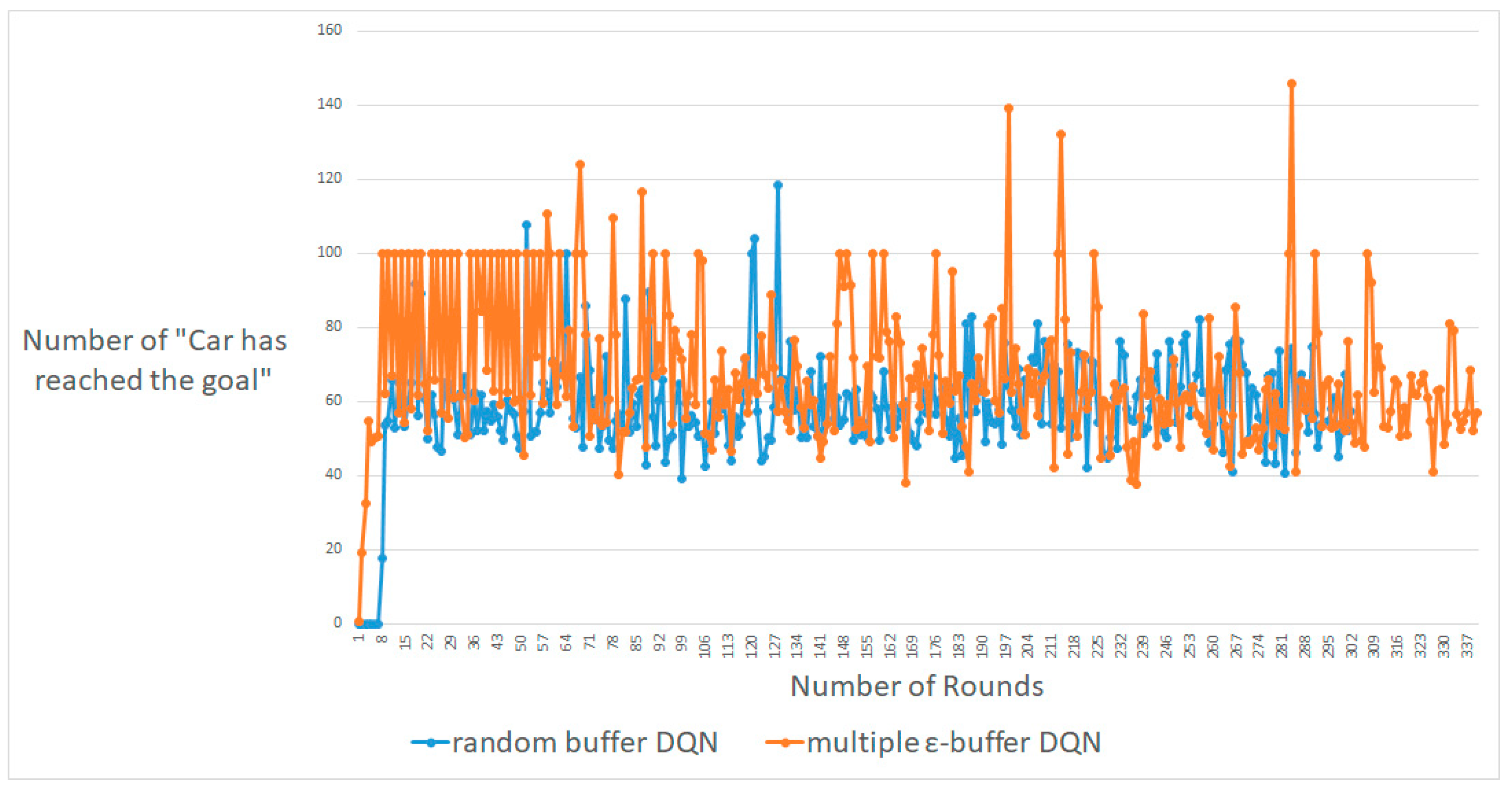
For DQN with multiple random ε-buffers, we follow similar previous studies [23]. Figure 5b shows a MountainCar-V0 [22] in OpenAI Gym [19]. Thus, GAMMA = 0.95, LEARNING − RATE = 0.001, MEMORY − SIZE = 100,000, BATCH − SIZE = 64, EXPLORATION − MAXIMUM = 1.0, EXPLORATION − MININUM = 0.01, and EXPLORATION − DECAY = 0.995 are the same as with previous DQN studies [23] because of a fairness comparison. In the MountainCar-V0 environment, there are two observations and three discrete actions, in Figure 6. Additionally, there are two episode terminations: when it reaches 0.5 position of the flag or if 200 iterations are reached. A penalty of 1 unit is applied for each move, including doing nothing. Our method limits the maximum number of times to 10,000 and 60 episodes by following the previous implementation of “Car has reached the goal” in each round [23].

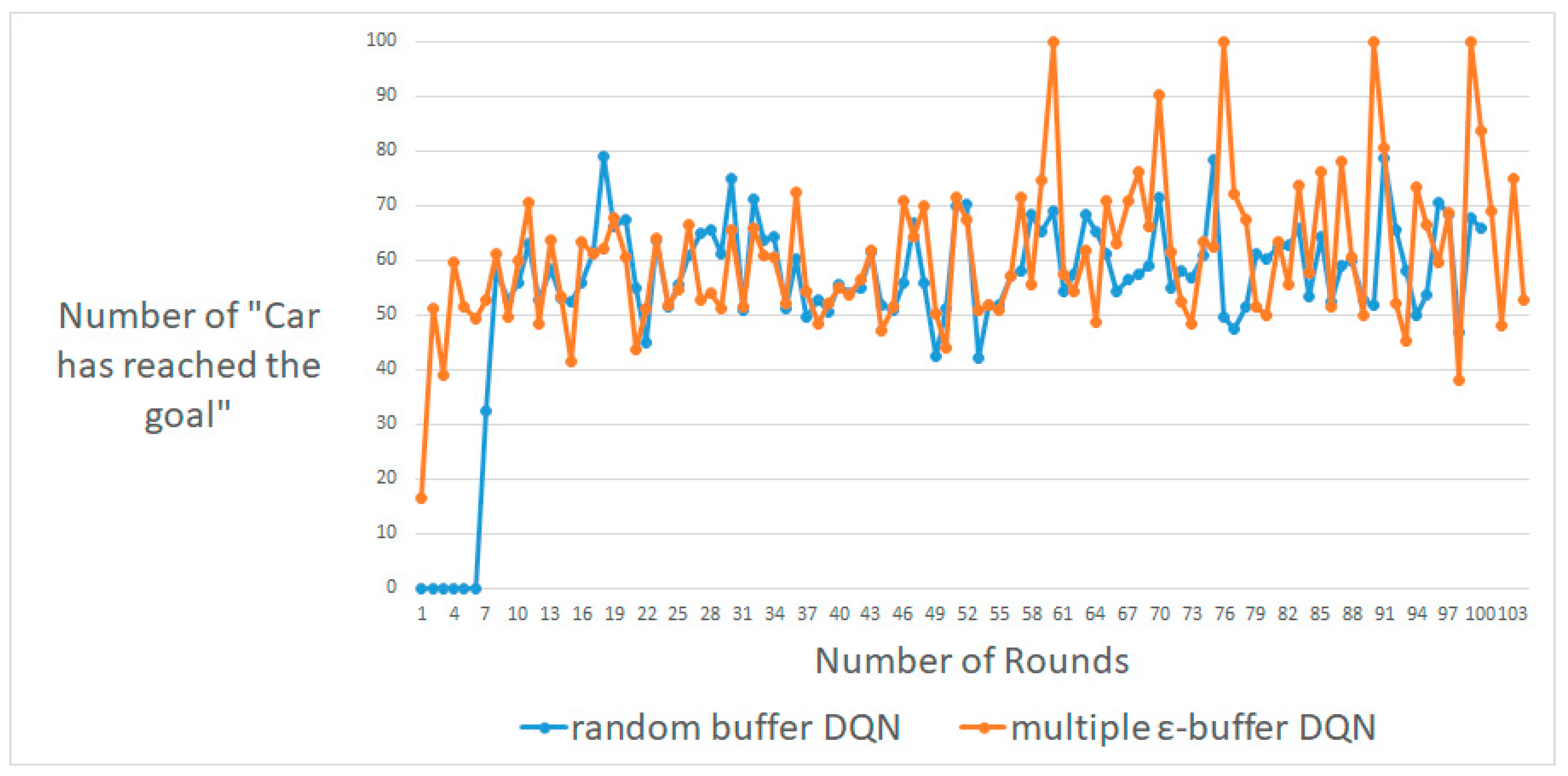
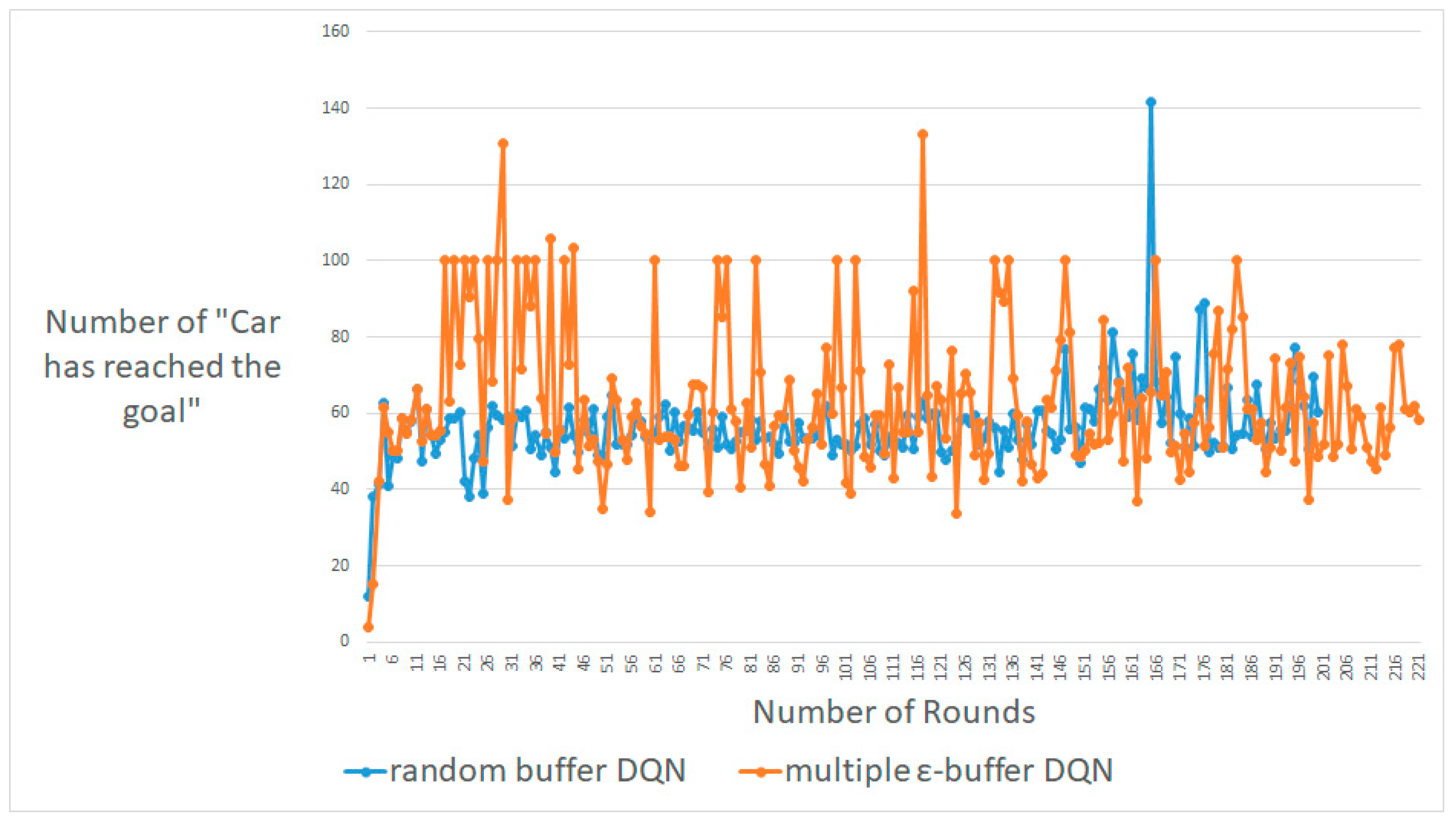
Figure 7, Figure 8 and Figure 9 display the maximum results for the number of rounds, from approximately 100 to 300. A DQN with multiple random ε-buffers can yield better results compared to when one random buffer is used. In each case, for around 100, 200 and 300 rounds, our proposed method shows that the number of “Car has reached the goal” [23] is higher than that obtained by DQN with one random buffer. We guarantee similar results for deep learning car simulations online, such as real-time learning with a normal neural network. Moreover, we can expect a real-time system with live training for real-time safeties. Similarly, for the experiment on Cart-Pole, we exploit the behavior policy to implement better exploration with multiple random ε-buffers so as not to follow a local minimum [9,10].

4.3. Pendulum-V0

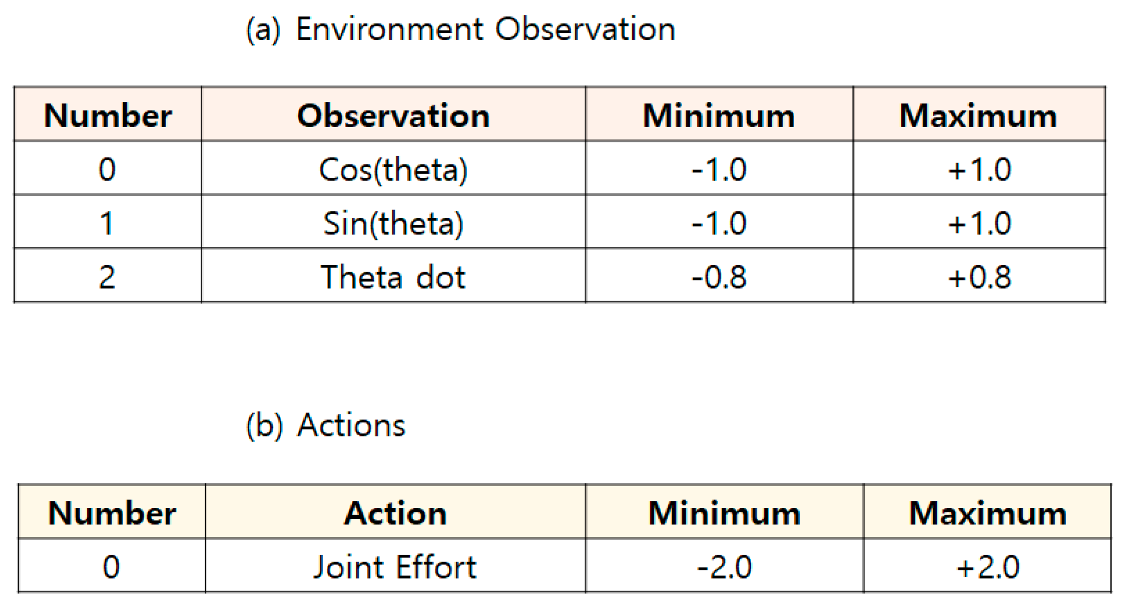
For DDPG with multiple random ε-buffers, we follow similar previous studies [25]. Figure 5c shows a Pendulum-V0 [24] by OpenAI Gym [19]. Thus, LEARNING − RATE = 0.001, MEMORY − SIZE = 2000, BATCH − SIZE = 32, EXPLORATION − MAXIMUM = 1.0, EXPLORATION − MINIMUM = 0.01, and EXPLORATION − DECAY = 1/2000 are the same as with the previous DQN studies [25] because of a fairness comparison. In the pendulum environment, there are three observations and one discrete action; see Figure 10. Additionally, there is a precise equation for the reward: −(θ² + 0.1 × θ² + 0.001 × action²), where θ is normalized between −π and +π. Therefore, the lowest cost is −(π² + 0.1 × 8² + 0.001 × 2²) = −16.2736044 and the highest cost is θ [25]. The goal is to remain at zero angle (vertical) with the least rotational velocity and least effort. There are no episode terminations, adding a maximum number of steps [24,25].

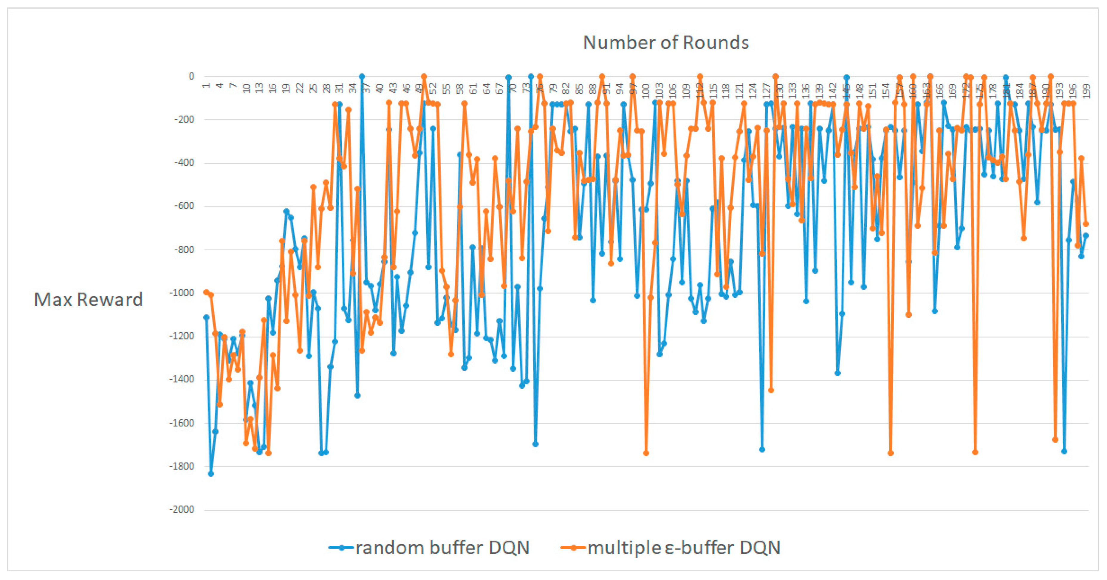
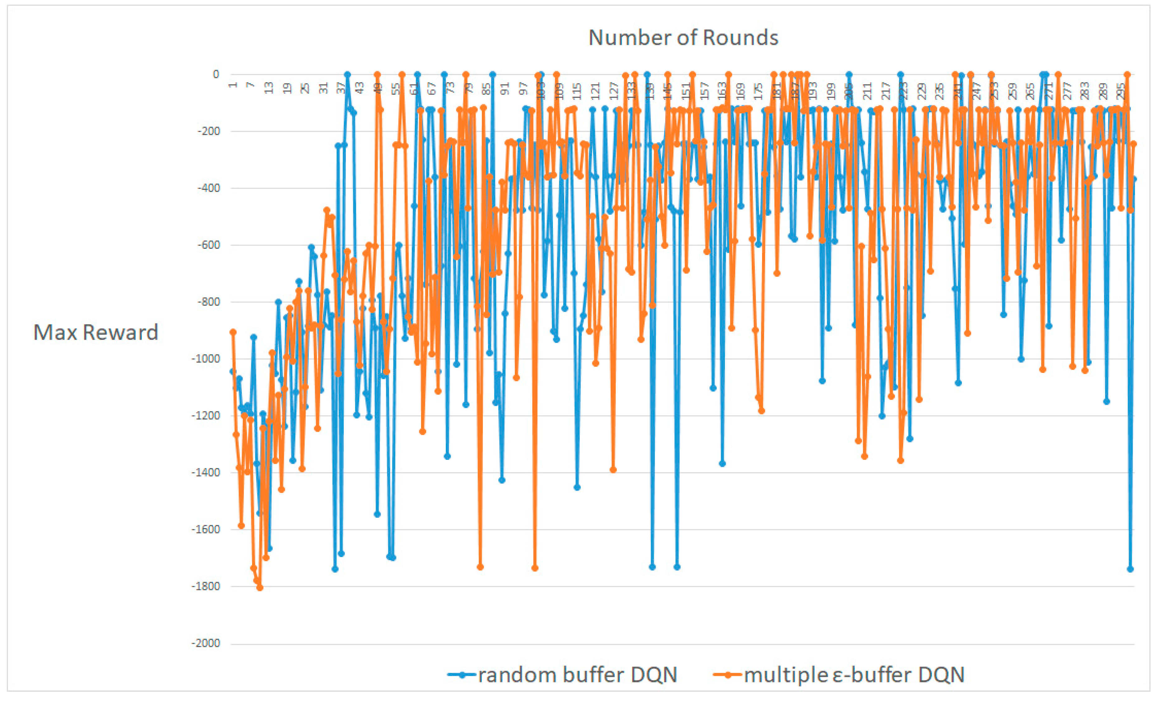
Figure 11, Figure 12 and Figure 13 exhibit the maximum results for the number of rounds, ranging from approximately 100–300. A DDPG with multiple random ε-buffers can yield a small improvement compared to that with one random buffer. In each case, for around 100, 200 and 300 rounds, our proposed method shows higher rewards than DDPG [16] with one random buffer. However, unlike the results of CartPole-V0 [20] and MountainCar-V0 [22], DDPG with multiple random ε-buffers cannot obtain a significant result compared with the cases of DQN. We consider this from the viewpoint of the on-policy. Fundamentally, a DDPG is based on the on-policy. Moreover, there is an issue about interpolating between policy optimization [2,16] and Q-learning [9,10]. The multiple random ε-buffers are actually based on Q-learning.

To train an agent, there are two major algorithms in model-free RL: policy optimization and Q-learning, which can follow the Bellman equation. A Q-learning agent selects an action to maximize the Q-value function based on the data at some point in the environment, regardless of the policy, known as the off-policy. Therefore, explorations on sample efficiency are extremely important to maximize the objective Q-value function. The representative algorithm in the off-policy is DQN. However, in terms of policy optimization, for better performance, an agent follows the recent deterministic policy and exploits a gradient ascent of the deterministic policy, thereby optimizing the parameters for the deterministic policy, known as the on-policy. Therefore, the update of the deterministic policy is extremely important for the exploration of the sample data. DDPG trains the agent by developing both the deterministic policy and the Q-value function. However, it is difficult to obtain both principled policy optimization and efficient Q-learning. That is why we cannot achieve better results in terms of DDPG. Therefore, we developed “Tradeoff Policy Optimization and Q-Learning” based on “Data vs. Policy” for better DDPG results. Thus, superior results can be obtained if we exploit a policy optimization method, based on the on-policy. This is another issue for future research.

5. Conclusions

We proposed multiple ε-greedy experience buffers in off-policy deep RL to enhance the exploration for superior and near-perfect generalization. We considered strengthening the advantages of explorations of model-free deep RL. We exploited multiple random ε-buffers for one original goal, and emulated the environment of OpenAI Gym to achieve better results in environments such as CartPole-V0, MountCar-V0, and Pendulum-V0. Our results demonstrated that the off-policy method was beneficial through an experimental comparison of DQN and DDPG based on on-policy. The proposed model is compatible with discrete actions as well as continuous control, symmetrically. Therefore, we can expect better prediction accuracy in real-time online learning, as in the detection of network intrusions through the verification of whether the network is “normal or anomalous.” Although our results are superior to those obtained by normal DQN with one random buffer, there is still scope for improvement, particularly for balancing policy optimization and Q-learning. The multiple random ε-buffers are fundamentally based on Q-learning. Therefore, the trade-offs between policy optimization and Q-learning should be solid and strong. Because of the deep neural network in RL, better results can be acquired in terms of DDPG, which is based on the on-policy of policy optimization. However, we can obtain better results if we develop another method based on policy optimization beyond the multiple random ε-buffers. The comparisons conducted in this study reveal that our model displays improvements in terms of exploration over the deep RL algorithms with Q-learning systems.

References

- Sutton, R.S.; Barto, A.G. Reinforcement Learning: An Introduction; MIT Press: Cambridge, MA, USA, 1998; Volume 1. [Google Scholar]
- Haarnoja, T.; Zhou, A.; Abbeel, P.; Levine, S. Soft Actor-Critic: Off-Policy Maximum Entropy Deep Reinforcement Learning with a Stochastic Actor. arXiv 2018, arXiv:1801.01290. [Google Scholar]
- Kim, C.; Park, J. Designing online network intrusion detection using deep auto-encoder Q-learning. Comput. Electr. Eng. 2019, 79, 106460. [Google Scholar] [CrossRef]
- Park, J.; Salim, M.M.; Jo, J.; Sicato, J.C.S.; Rathore, S.; Park, J.H. CIoT-Net: A scalable cognitive IoT based smart city network architecture. Hum. Cent. Comput. Inf. Sci. 2019, 9, 29. [Google Scholar] [CrossRef]
- Sun, Y.; Tan, W. A trust-aware task allocation method using deep q-learning for uncertain mobile crowdsourcing. Hum. Cent. Comput. Inf. Sci. 2019, 9, 25. [Google Scholar] [CrossRef] [Green Version]
- Kwon, B.-W.; Sharma, P.K.; Park, J.-H. CCTV-Based Multi-Factor Authentication System. J. Inf. Process. Syst. JIPS 2019, 15, 904–919. [Google Scholar] [CrossRef]
- Srilakshmi, N.; Sangaiah, A.K. Selection of Machine Learning Techniques for Network Lifetime Parameters and Synchronization Issues in Wireless Networks. Inf. Process. Syst. JIPS 2019, 15, 833–852. [Google Scholar] [CrossRef]
- Andrychowicz, M.; Wolski, F.; Ray, A.; Schneider, J.; Fong, R.; Welinder, P.; McGrew, B.; Tobin, J.; Abbeel, P.; Zaremba, W. Hindsight Experience Replay. arXiv 2017, arXiv:1707.01495. [Google Scholar]
- Mnih, V.; Kavukcuoglu, K.; Silver, D.; Graves, A.; Antonoglou, I.; Wierstra, D.; Riedmiller, M. Playing atari with deep reinforcement learning. arXiv 2013, arXiv:1312.5602. [Google Scholar]
- Silver, D.; Huang, A.; Maddison, C.J.; Guez, A.; Sifre, L.; Driessche, G.V.D.; Schrittwieser, J.; Antonoglou, I.; Panneershelvam, V.; Lanctot, M. Mastering the game of go with deep neural networks and tree search. Nature 2016, 529, 484–489. [Google Scholar] [CrossRef] [PubMed]
- Cobbe, K.; Klimov, O.; Hesse, C.; Kim, T.; Schulman, J. Quantifying Generalization in Reinforcement Learning. arXiv 2019, arXiv:1812.02341. [Google Scholar]
- Liu, R.; Zou, J. The Effects of Memory Replay in Reinforcement Learning. arXiv 2017, arXiv:1710.06574. [Google Scholar]
- Schaul, T.; Quan, J.; Antonoglou, I.; Silver, D. Prioritized Experience Replay. arXiv 2016, arXiv:1511.05952. [Google Scholar]
- Plappert, M.; Houthooft, R.; Dhariwal, P.; Sidor, S.; Chen, R.; Chen, X.; Asfour, T.; Abbeel, P.; Andrychowicz, M. Parameter Space Noise for Exploration. arXiv 2018, arXiv:1706.01905. [Google Scholar]
- OpenReview.net. Available online: https://openreview.net/forum?id=ByBAl2eAZ (accessed on 16 February 2018).
- Lillicrap, T.; Hunt, J.; Pritzel, A.; Heess, N.; Erez, T.; Tassa, Y.; Silver, D.; Wierstra, D. Continuous control with deep reinforcement learning. arXiv 2016, arXiv:1509.02971. [Google Scholar]
- FreeCodeCamp. Available online: https://medium.freecodecamp.org/improvements-in-deep-q-learning-dueling-double-dqn-prioritized-experience-replay-and-fixed-58b130cc5682 (accessed on 5 July 2018).
- RL—DQN Deep Q-network. Available online: https://medium.com/@jonathan_hui/rl-dqn-deep-q-network-e207751f7ae4 (accessed on 17 July 2018).
- OpenAI Gym. Available online: https://gym.openai.com (accessed on 28 May 2016).
- Cart-Pole-V0. Available online: https://github.com/openai/gym/wiki/Cart-Pole-v0 (accessed on 24 June 2019).
- Cart-Pole-DQN. Available online: https://github.com/rlcode/reinforcement-learning-kr/blob/master/2-cartpole/1-dqn/cartpole_dqn.py (accessed on 8 July 2017).
- MountainCar-V0. Available online: https://github.com/openai/gym/wiki/MountainCar-v0 (accessed on 4 May 2019).
- MountainCar-V0-DQN. Available online: https://github.com/shivaverma/OpenAIGym/blob/master/mountain-car/MountainCar-v0.py (accessed on 2 April 2019).
- Pendulum-V0. Available online: https://github.com/openai/gym/wiki/Pendulum-v0 (accessed on 31 May 2019).
- Pendulum-V0-DDPG. Available online: https://github.com/openai/gym/blob/master/gym/envs/classic_control/pendulum.py (accessed on 26 October 2019).
- Tensorflow. Available online: https://github.com/tensorflow/tensorflow (accessed on 31 October 2019).
- Keras Documentation. Available online: https://keras.io/ (accessed on 14 October 2019).
Figure 2.
(a) The environment of CartPole-V0 and (b) the actions taken by the agent of CartPole-V0 [20].
Figure 3.
An average result between DQN with random buffers and DQN with multiple random ε-buffers in CartPole-V0.
Figure 4.
One of the best results between DQN with random buffers and DQN with multiple random ε-buffers in CartPole-V0.
Figure 5.
One of the worst results between DQN with random buffers and DQN with multiple random ε-buffers in CartPole-V0.
Figure 6.
(a) The environment of MountainCar-V0 and (b) the actions taken by the agent of MountainCar-V0 [22].
Figure 7.
Maximum number of rounds, i.e., around 100, between DQN with random buffers and DQN with multiple random ε-buffers in MountainCar-V0.
Figure 8.
Maximum number of rounds, i.e., around 200, between DQN with random buffers and DQN with multiple random ε-buffers in MountainCar-V0.
Figure 9.
The maximum number of rounds, i.e., around 300, between DQN with random buffers and DQN with multiple random ε-buffers in MountainCar-V0.
Figure 10.
(a) The environment of MountainCar-V0 and (b) the actions taken by the agent of Pendulum-V0 [24].
Figure 11.
Maximum number of rounds, i.e., around 100, between DDPG with random buffers and DQN with multiple random ε-buffers in MountainCar-V0.
Figure 12.
Maximum number of rounds, i.e., around 200, between DDPG with random buffers and DQN with multiple random ε-buffers in MountainCar-V0.
Figure 13.
Maximum number of rounds, i.e., around 300, between DDPG with random buffers and DQN with multiple random ε-buffers in MountainCar-V0.
© 2019 by the authors. Licensee MDPI, Basel, Switzerland. This article is an open access article distributed under the terms and conditions of the Creative Commons Attribution (CC BY) license (http://creativecommons.org/licenses/by/4.0/).
Share and Cite
MDPI and ACS Style
Kim, C.; Park, J. Exploration with Multiple Random ε-Buffers in Off-Policy Deep Reinforcement Learning. Symmetry 2019, 11, 1352. https://doi.org/10.3390/sym11111352
AMA Style
Kim C, Park J. Exploration with Multiple Random ε-Buffers in Off-Policy Deep Reinforcement Learning. Symmetry. 2019; 11(11):1352. https://doi.org/10.3390/sym11111352
Chicago/Turabian StyleKim, Chayoung, and JiSu Park. 2019. "Exploration with Multiple Random ε-Buffers in Off-Policy Deep Reinforcement Learning" Symmetry 11, no. 11: 1352. https://doi.org/10.3390/sym11111352
Note that from the first issue of 2016, this journal uses article numbers instead of page numbers. See further details here.