Exponentiation in QED and Quasi-Stable Charged Particles

Abstract

In this note we present a new exponentiation scheme of soft photon radiation from charged quasi-stable resonances. It generalizes the well established scheme of Yennie, Frautschi and Suura. While keeping the same functional form of an exponent, the new scheme is both exact in its soft limit and accounts properly for the kinematical shift in resonant propagators. We present the scheme on an example of two processes: a toy model of single W production in $e\nu$ scattering and the W pair production and decay in $e^{+}{e}^{-}$ annihilation. The latter process is of relevance for the planned FCCee collider where high precision of Monte Carlo simulations is a primary goal. The proposed scheme is a step in this direction.

1. Introduction

Emission of soft photons accompany every process with charged particles. Therefore proper treatment of such emission is mandatory. These emissions happen from the external particles, decouple from the process itself and can be resummed and exponentiated in an universal way [1]. In such an approach the information on the photonic emission is not transmitted to the process itself. This can pose a problem if the process includes resonant particles in the intermediate state, because any energy loss due to photonic emission, larger compared to the width of the resonance can shift the process off resonance and the Γ/M suppression should be visible. We will refer to it as the recoil effect. This effect for the case of neutral resonance has been resolved with the help of coherent states in References [2,3], and then at the level of spin amplitudes in Reference [4].

In the case of charged resonances another complication appears: the resonance is a source of the soft photons as well. Of course, strictly speaking, the internal particles do not radiate soft photons (do not have singularities due to such radiation), as demonstrated by Yennie, Frautschi and Suura (YFS61) in the classical Reference [1]. However, the resonances are special – they are quasi-stable and there is a clear separation between their production and decay. One can illustrate it with the case of lepton $\tau$ for which the lifetime is longer than the time-scale of the production by an astronomical factor of $m_{\tau }/{\mathsf{\Gamma }}_{\tau }\simeq 3\times {10}^{11}$. Resummation (exponentiation) of such emissions is the subject of this note. We will present a solution that smoothly interpolates between two situations: for $\sum k^0<\mathsf{\Gamma }$ we have the normal YFS61 behaviour, i.e. internal radiation is suppressed, whereas for $\sum k^0>\mathsf{\Gamma }$ the recoil effect is properly accounted for. More details can be found in a recent paper [5].

We analyse two processes: the simplest toy model, $e{\overline{\nu }}_e\to W\to \mu {\overline{\nu }}_{\mu }$, on which we demonstrate the methodology; and with an eye on future $e^{+}{e}^{-}$ collider, the full-scale process, $e^{+}{e}^{-}\to WW\to 4f$. The latter process is one of a few gold-plated processes of the projected FCCee machine. In its second phase, at the $WW$-threshold, the FCCee would provide about $3\times {10}^7$ $WW$ events. That number corresponds to a statistical error on the total cross section of 0.02%, or equivalently $\Delta M_W\simeq 0.3$ MeV (measured from the threshold scan). The current state of the art, inherited from the LEP2 era, is 0.5–2% for the total cross section. That means, an increase of the precision by factor of 100 is needed. The most important part of that challenge is to calculate the $\mathcal{O}\left({\alpha }^2\right)$ corrections to the signal process $e^{+}{e}^{-}\to WW\to 4f$. Exponentiation of soft radiation from Ws, which is equivalent to resummation (exact in the soft limit) of photon interferences between production and decay stages as well as between decays of the two Ws would encapsulate an important part of these corrections, not only to the second order but to all orders!

There is also another, practical, and perhaps even most important, application of the soft YFS-based exponentiation—the Monte Carlo event generators. The whole familly of such generators has emerged from the never published note of S. Jadach [6]. All of them generate multiple sof-photon emissions based on the classical YFS61 exponentiation. Among them one should list BHLUMI [7] and KORALZ [8]. The latter one has been then replaced by a next-generation-code KKMC [9] which includes recoil in production-decay interferences of the Z-resonance. The partial solutions related to the charged W bosons have been implemented in the YFSWW3 program [10] where exponentiation of the emission in the $WW$ pair production ($ee\to WW$) with the recoil has been done and in WINHAC [11] in which exponentiation of radiation in the W decay ($W\to f_1{f}_2$) is implemented for the single-W process.

At last, let us only touch upon the issue of QED deconvolution. The YFS approach provides for a very convenient scheme of such a deconvolution also in higher orders. When supplied with the treatment of resonances, it would form a complete and well defined deconvolution system.

The paper is organized as follows. In Section 2 we present the standard YFS scheme and its new extension on the example of the simple “toy model” $e{\overline{\nu }}_e\to W\to \mu {\overline{\nu }}_{\mu }$. In Section 3 we discuss the exponentiation in the process of W-pair production and decay. In particular we show how to introduce virtual soft-photon interferences and how to exponentiate them. The last section contains conclusions and summary.

2. Toy Model with Single W

In this section we show, in the combinatorial language, on the simplest possible example of $e\left(p_a\right){\overline{\nu }}_e\left(p_b\right)\to W\to \mu \left(p_c\right){\overline{\nu }}_{\mu }\left(p_d\right)$, how the YFS61 procedure works and then we extend it by adding the soft real emission from the semi-stable W boson. The combinatorial resummation presented here differs from the original YFS61 derivation of Ref. [1] which was done with the help of Bose symmetry principles.

2.1. Classical YFS Resummation from External Legs

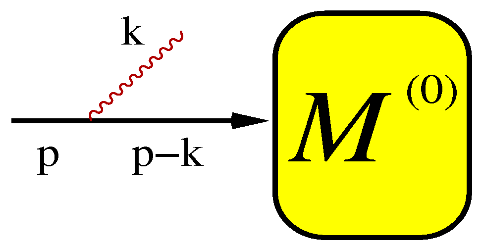
The YFS61 theorem states that soft emissions are singular only from external legs. For the single emission in a generic process $\mathcal{M}$, depicted in Figure 1 we have

$${\mathcal{M}}^{\mu }\simeq {\mathcal{M}}^{\left(0\right)}(p-k)\frac{\mathbf{p}-\mathbf{k}+m}{k^2-2kp+i\epsilon }{\gamma }^{\mu }{u}_p\stackrel{k\to 0}{=}\frac{2p^{\mu }-k^{\mu }}{k^2-2kp+i\epsilon }{\mathcal{M}}^{\left(0\right)}\left(p\right)u_p.$$

(1)

This way the soft-photon current $\frac{2p^{\mu }-k^{\mu }}{k^2-2kp+i\epsilon }$ (either real or virtual) decouples from the hard process $\mathcal{M}$.

Let us now consider the toy-model situation shown in Figure 2. This figure corresponds to the following expression in which we have omitted all the details except for the photonic radiation in the soft approximation and the propagator of the resonance (mass M includes width Γ):

$$\begin{array}{c}{{\mathcal{M}}_N^{\left(0\right)}}^{{\mu }_1,\cdots ,{\mu }_N}(k_1,\cdots ,k_N)\simeq \hfill \\ \simeq {\displaystyle \sum _{l=0}^N}{\displaystyle \sum _{\pi }^{N!}}\left(\frac{2p_a^{{\mu }_1}}{2p_a{k}_{{\pi }_1}}\frac{2p_a^{{\mu }_2}}{2p_a{k}_{{\pi }_1}+2p_a{k}_{{\pi }_2}}\cdots \frac{2p_a^{{\mu }_l}}{2p_a{k}_{{\pi }_1}+2p_a{k}_{{\pi }_2}+\cdots +2p_a{k}_{{\pi }_l}}\right)\hfill \\ \times \left(\frac{-2p_c^{{\mu }_{l+1}}}{2p_c{k}_{{\pi }_{l+1}}}\frac{-2p_c^{{\mu }_{l+2}}}{2p_c{k}_{{\pi }_{l+1}}+2p_c{k}_{{\pi }_{l+2}}}\cdots \frac{-2p_c^{{\mu }_N}}{2p_c{k}_{{\pi }_{l+1}}+2p_c{k}_{{\pi }_{l+2}}+\cdots +2p_c{k}_{{\pi }_N}}\right)\hfill \\ \times \frac{1}{p_{cd}^2-M^2}.\hfill \end{array}$$

(2)

The index l corresponds to the number of photons in the initial state (a) and $\pi$ denotes a permutation of photons. In the first step we use the well known algebraical formula

$$\begin{array}{c}\hfill {\displaystyle \sum _{perm.}}\frac{1}{p{k}_1(p{k}_1+p{k}_2)\cdots (p{k}_1+p{k}_2+\cdots p{k}_n)}=\frac{1}{p{k}_{1}p{k}_2\cdots p{k}_n}\end{array}$$

(3)

to get

$$\begin{array}{c}{{\mathcal{M}}_N^{\left(0\right)}}^{{\mu }_1,\cdots ,{\mu }_N}(k_1,\cdots ,k_N)\simeq \frac{1}{p_{cd}^2-M^2}{\displaystyle \sum _{l=0}^N}{\displaystyle \sum _{\pi /{\pi }_l/{\pi }_{N-l}}^{N!/l!/(n-l)!}}\left({\displaystyle \prod _{i=1}^l}\frac{2p_a^{{\mu }_i}}{2p_a{k}_{{\pi }_i}}\right)\left({\displaystyle \prod _{i=1}^{N-l}}\frac{-2p_c^{{\mu }_{l+i}}}{2p_c{k}_{{\pi }_{l+i}}}\right).\hfill \end{array}$$

(4)

The expression $\pi /{\pi }_l/{\pi }_{N-l}$ means that summation over separate permutations within the initial and final photon subgroups has been carried out. The leftover sum over permutations can be rearranged now into the sum over partitions ${\wp }_i$ in which each photon is labelled only as initial (a) or final (c):

$$\begin{array}{c}{\displaystyle \sum _{\genfrac{}{}{0pt}{}{l_a,l_c=0}{l_a+l_c=n}}^n}{\displaystyle \sum _{\pi /{\pi }_a/{\pi }_b/{\pi }_c}^{n!/l_a!/l_c!}}={\displaystyle \sum _{\wp ={(a,c)}^n}^{2^n}}.\end{array}$$

(5)

This brings us to the final result:

$$\begin{array}{c}{{\mathcal{M}}_N^{\left(0\right)}}^{{\mu }_1,\cdots ,{\mu }_N}(k_1,\cdots ,k_N)\simeq \frac{1}{p_{cd}^2-M^2}{\displaystyle \sum _{\wp ={(a,c)}^N}^{2^N}}\left({\displaystyle \prod _{i=1}^N}\frac{2{\theta }_{{\wp }_i}{p}_{{\wp }_i}^{{\mu }_i}}{2p_{{\wp }_i}{k}_i}\right).\hfill \end{array}$$

(6)

The ${\theta }_i$ is equal to $+1(-1)$ for the initial (final) photon. The formula (6) can also be conveniently rewritten by turning the sum over partitions into a product, e.g., for two photons we have:

$$\begin{array}{c}\hfill \frac{p_a^{{\mu }_1}}{p_a{k}_1}\frac{p_a^{{\mu }_2}}{p_a{k}_2}-\frac{p_a^{{\mu }_1}}{p_a{k}_1}\frac{p_c^{{\mu }_2}}{p_c{k}_2}-\frac{p_c^{{\mu }_1}}{p_c{k}_1}\frac{p_a^{{\mu }_2}}{p_a{k}_2}+\frac{p_c^{{\mu }_1}}{p_c{k}_1}\frac{p_c^{{\mu }_2}}{p_c{k}_2}=\left(\frac{p_a^{{\mu }_1}}{p_a{k}_1}-\frac{p_c^{{\mu }_1}}{p_c{k}_1}\right)\left(\frac{p_a^{{\mu }_2}}{p_a{k}_2}-\frac{p_c^{{\mu }_2}}{p_c{k}_2}\right).\end{array}$$

(7)

This way we obtain the formula in the form of YFS61:

$${{\mathcal{M}}_N^{\left(0\right)}}^{{\mu }_1,\cdots ,{\mu }_N}(k_1,\cdots ,k_N)\simeq {\displaystyle \prod _{i=1}^N}\left(\frac{2p_a^{{\mu }_i}}{2p_a{k}_i}-\frac{2p_c^{{\mu }_i}}{2p_c{k}_i}\right).$$

(8)

Squaring and integrating over $k_i$ with the $1/N!$ Bose–Einstein symmetry factor leads us to the desired exponential form. Note that, contrary to Equation (6), the formula (8) will not be valid when the recoil effect is included, see below for more comments.

2.2. Inclusion of Emission from W Boson

Now let us extend the analysis to the situation depicted in Figure 3. We include multiple emission of $l_n$ soft photons from an internal W line. Emissions are connected by the W propagators. If we consider a product of two W propagators we find that it can be rewritten as a sum of two terms, each of them being a product of a single W propagator and the soft-photon emission factor before or after the W.

$$\begin{array}{c}\frac{1}{(Q_0^2-M^2)}\frac{1}{(Q_1^2-M^2)}=\frac{1}{(Q_0^2-Q_1^2)(Q_1^2-M^2)}-\frac{1}{(Q_0^2-M^2)(Q_0^2-Q_1^2)}\\ =\frac{1}{(2k_1{Q}_0-k_1^2)(Q_1^2-M^2)}-\frac{1}{(Q_0^2-M^2)(2k_1{Q}_1+k_1^2)}.\end{array}$$

(9)

That formula has a simple physical interpretation: soft emission belongs either to production or to decay phase and the W propagator knows it because its four-momentum is correctly adjusted (recoil effect). We can now generalize it to $l_n$ emissions shown in Figure 3:

$$\begin{array}{c}{\displaystyle \sum _{permut.}}\frac{1}{(Q_0^2-M^2)(Q_1^2-M^2)\cdots (Q_{l_n}^2-M^2)}\hfill \\ ={\displaystyle \sum _{{\wp =(P,D)}^{ln}}}{\displaystyle \prod _{{\wp }_i=P}}\frac{1}{{(Q_{\wp }+k_i)}^2-Q_{\wp }^2}\times \frac{1}{Q_{\wp }^2-M^2}\times {\displaystyle \prod _{{\wp }_i=D}}\frac{1}{{(Q_{\wp }+k_i)}^2-Q_{\wp }^2},\hfill \end{array}$$

(10)

where $Q\wp =Q_0-{\displaystyle \sum _{{\wp }_i=P}}{k}_i=Q_{l_n}+{\displaystyle \sum _{{\wp }_i=D}}{k}_i.$ As before, the physical picture, illustrated in Figure 4, is clear: a set of soft emissions (interpreted as belonging to the production process) precedes the W propagator and a second set (interpreted as belonging to the decay process) follows it. The recoil is properly included in the W propagator.

As for the numerators of the W propagators, in the soft limit and in the on-shell approximation (numerators are mild functions of momenta, so accounting for the recoil is not needed), we find

$$\begin{array}{c}{D}_W\left(p\right)V{(p,k,p-k)}_{\rho }{D}_W\left(p\right)\stackrel{k\to 0,p^2\to M_W^2}{=}{D}_W\left(p\right)(-2p_{\rho }),\hfill \end{array}$$

(11)

where $V{(p,k,p-k)}_{\rho }$ is the $W\gamma W$ vertex and $D_W\left(p\right)$ denotes the numerator of the W propagator. For more emissions Equation (11) has a self-repeating structure and reduces multiple emissions into numerators of the soft factors, i.e., ${\prod }_{i}2p_{{\rho }_i}$.

Combining Equation (2) with (10) and (11) we can write down the formula that corresponds to Figure 4:

$$\begin{array}{c}{{\mathcal{M}}_N^{\left(0\right)}}^{{\mu }_1,\cdots ,{\mu }_N}(k_1,\cdots ,k_N)\simeq {\displaystyle \sum _{\genfrac{}{}{0pt}{}{l_a,l_c,n=0}{l_a+l_c+n=N}}^N}{\displaystyle \sum _{\genfrac{}{}{0pt}{}{l_g,l_h=0}{l_g+l_h=n}}^n}{\displaystyle \sum _{\pi }^{N!}}\hfill \end{array}$$

(12)

$$\begin{array}{c}[\left(\frac{2p_a^{{\mu }_{{\pi }_1}}}{2p_a{k}_{{\pi }_1}}\frac{2p_a^{{\mu }_{{\pi }_2}}}{2p_a{k}_{{\pi }_1}+2p_a{k}_{{\pi }_2}}\cdots \frac{2p_a^{{\mu }_{{\pi }_{l_a}}}}{2p_a{k}_{{\pi }_1}+2p_a{k}_{{\pi }_2}+\cdots +2p_a{k}_{{\pi }_{l_a}}}\right)\hfill \end{array}$$

(13)

$$\begin{array}{c}\left(\frac{-2Q_{{\pi }_0}^{{\mu }_{{\pi }_{l_a+1}}}}{2Q_{{\pi }_{l_g}}{k}_{{\pi }_{l_a+1}}}\frac{-2Q_{{\pi }_0}^{{\mu }_{{\pi }_{l_a+2}}}}{2Q_{{\pi }_{l_g}}{k}_{{\pi }_{l_a+1}}+2Q_{{\pi }_{l_g}}{k}_{{\pi }_{l_a+2}}}\cdots \frac{-2Q_{{\pi }_0}^{{\mu }_{{\pi }_{l_a+l_g}}}}{2Q_{{\pi }_{l_g}}{k}_{{\pi }_{l_a+1}}+2Q_{{\pi }_{l_g}}{k}_{{\pi }_{l_a+2}}+\cdots +2Q_{{\pi }_{l_g}}{k}_{{\pi }_{l_a+l_g}}}\right)\hfill \end{array}$$

(14)

$$\begin{array}{c}\frac{D_W\left(Q_{{\pi }_{l_g}}\right)}{Q_{{\pi }_{l_g}}^2-M_W^2}\hfill \end{array}$$

(15)

$$\begin{array}{c}(\frac{2Q_{{\pi }_0}^{{\mu }_{{\pi }_{l_a+l_g+1}}}}{2Q_{{\pi }_{l_g}}{k}_{{\pi }_{l_a+l_g+1}}}\frac{2Q_{{\pi }_0}^{{\mu }_{{\pi }_{l_a+l_g+2}}}}{2Q_{{\pi }_{l_g}}{k}_{{\pi }_{l_a+l_g+1}}+2Q_{{\pi }_{l_g}}{k}_{{\pi }_{l_a+l_g+2}}}\cdots \hfill \end{array}$$

(16)

$$\begin{array}{c}\frac{2Q_{{\pi }_0}^{{\mu }_{{\pi }_{l_a+l_g+l_h}}}}{2Q_{{\pi }_{l_g}}{k}_{{\pi }_{l_a+l_g+1}}+2Q_{{\pi }_{l_g}}{k}_{{\pi }_{l_a+l_g+2}}+\cdots +2Q_{{\pi }_{l_g}}{k}_{{\pi }_{l_a+l_g+l_h}}})\hfill \end{array}$$

(17)

$$\begin{array}{c}\left(\frac{-2p_c^{{\mu }_{{\pi }_{l_a+n+1}}}}{2p_c{k}_{{\pi }_{l_a+n+1}}}\frac{-2p_c^{{\mu }_{{\pi }_{l_a+n+2}}}}{2p_c{k}_{{\pi }_{l_a+n+1}}+2p_c{k}_{{\pi }_{l_a+n+2}}}\cdots \frac{-2p_c^{{\mu }_{{\pi }_{l_a+n+l_c}}}}{2p_c{k}_{{\pi }_{l_a+n+1}}+2p_c{k}_{{\pi }_{l_a+n+2}}+\cdots +2p_c{k}_{{\pi }_{l_a+n+l_c}}}\right)].\hfill \end{array}$$

(18)

Let us explain this long formula. Lines (13) and (18) describe the standard YFS emission from the external legs a and c, whereas lines (14), (16) and (17) describe the emissions from the W-boson. It is important that both groups have identical structure and we can re-interpret them as the standard YFS emission in the production phase (lines (13) and (14)) and in the decay (lines (16) and (18)). Standard resummations can now be performed separately on the production and on the decay in complete analogy to Equation (8).

This is possible because the recoil does not depend separately on photons from electron (muon) and from the W boson, but only on their sum.

The production and decay parts are still interconnected by the sum over partitions of photons between production and decay of the form of Equation (6). This leads to the final formula

$$\begin{array}{c}{\mathcal{M}}_N^{\left(0\right)}\simeq {\displaystyle \sum _{\wp ={(P,D)}^N}^{2^N}}\frac{D_W\left(Q_g\right)}{Q_g^2-M_W^2}{\displaystyle \prod _{i=1}^N}{j}_{{\wp }_i}^{{\mu }_i},\hfill \\ j_P^{{\mu }_i}=\frac{2p_a^{{\mu }_i}}{2p_a{k}_i}-\frac{2Q_g^{{\mu }_i}}{2Q_g{k}_i},j_D^{{\mu }_i}=\frac{2Q_g^{{\mu }_i}}{2Q_g{k}_i}-\frac{2p_c^{{\mu }_i}}{2p_c{k}_i},Q_g=p_{cd}+{\displaystyle \sum _{decay}}{k}_i.\hfill \end{array}$$

(19)

${\sum }_{\wp ={(P,D)}^N}^{2^N}$ is a sum over partitions of photons emitted in the production and in the decay.

3. W-Pair Production and Decay

Having explained in very detail the resummation of the real emission in the toy model, we now proceed briefly to the resummation in the W-pair production and decay process. Let us include virtual photons into the formulae. In the case of YFS61, shown on LHS of Figure 5, their resummation goes in complete analogy to the real photons, and the appropriate formula for m real photons and an arbitrary number of virtual ones, for 6 external particles, reads:

$$\begin{array}{cc}\hfill M^{{\mu }_1{\mu }_2\dots {\mu }_m}& (k_1,k_2,\cdots ,k_m)=\hfill \\ & =\mathcal{M}{\displaystyle \prod _{l=1}^m}{j}^{{\mu }_l}\left(k_l\right){\displaystyle \sum _{n=0}^{\infty }}\frac{1}{n!}{\displaystyle \prod _{i=1}^n}\int \frac{i}{{\left(2\pi \right)}^3}\frac{d^4{k}_i}{k_i^2-{\lambda }^2+i\epsilon }{J}_6^{\mu }\left(k_i\right)x\circ J_{6\mu }\left(k_i\right)\hfill \\ & =\mathcal{M}{\displaystyle \prod _{l=1}^m}{j}^{{\mu }_l}\left(k_l\right)e^{\alpha B_6},\hfill \\ \hfill B_6& =\int \frac{i}{{\left(2\pi \right)}^3}\frac{d^{4}k}{k^2-{\lambda }^2+i\epsilon }{J}_6\left(k\right)\circ J_6\left(k\right),\hfill \end{array}$$

(20)

where

$$\begin{array}{c}{J}_6^{\mu }\left(k\right)={\displaystyle \sum _{X=a,b,c,d,e,f}}{\hat{J}}_X^{\mu }\left(k\right),\hfill \\ {\widehat{J}}_X^{\mu }\left(k\right)\equiv Q_X{\theta }_X\frac{2p_X^{\mu }{\theta }_X-k^{\mu }}{k^2-2p_{X}k{\theta }_X+i\epsilon },\hfill \\ J_X\left(k\right)\circ J_Y\left(k\right)=J_X\left(k\right)J_Y(-k)\mathrm{for}X\ne Y,J_X\left(k\right)\circ J_X\left(k\right)=J_X\left(k\right)J_X\left(k\right).\hfill \end{array}$$

(21)

The real soft-photon emissions have the familiar form of a product of the currents $j^{{\mu }_l}\left(k_l\right)$, and the similar virtual soft-photon currents $J^{\mu }\left(k\right)$ are resummed.

Let us now proceed to a new, extended scheme. That scheme is illustrated on RHS of Figure 5. We have additional real soft-photon emissions from Ws as well as all virtual soft-photon interferences between the production and two decays. The resummation of real emissions proceeds exactly as in the toy example as a product of currents. The virtual soft-photon emissions follow the same logics and formulae as the real ones. The only exceptions are the issues related to the definition of the mass and width of the resonance and the UV renormalisation. Analysis of these issues is beyond the scope of this paper. Here we make an educated guess based on the solid principle of the cancellation of soft-photon singularities in QED and propose the following formula for a given partition of real momenta $k_{i_1},k_{i_2},k_{i_3}$

$$\begin{array}{c}{M}_{n_1{n}_2{n}_3}^{{\mu }_{1_1}\cdots {\mu }_{3_{n_3}}}\left(\left\{k\right\}\right)={\mathcal{M}}_0{\displaystyle \prod _{i_1=1}^{n_1}}{j}_P^{{\mu }_{i_1}}\left(k_{i_1}\right){\displaystyle \prod _{i_2=1}^{n_2}}{j}_{D_1}^{{\mu }_{i_2}}\left(k_{i_2}\right){\displaystyle \prod _{i_3=1}^{n_3}}{j}_{D_2}^{{\mu }_{i_3}}\left(k_{i_3}\right)\times \hfill \\ {\displaystyle \sum _{n_4=0}^{\infty }}\frac{1}{n_4!}{\displaystyle \prod _{i_4=1}^{n_4}}\int \frac{i}{{\left(2\pi \right)}^3}\frac{d^4{k}_{i_4}}{k_{i_4}^2-m_{\gamma }^2+i\epsilon }{J}_P\left(k_{i_4}\right)\circ J_P\left(k_{i_4}\right)\hfill \\ {\displaystyle \sum _{n_5=0}^{\infty }}\frac{1}{n_5!}{\displaystyle \prod _{i_5=1}^{n_5}}\int \frac{i}{{\left(2\pi \right)}^3}\frac{d^4{k}_{i_5}}{k_{i_5}^2-m_{\gamma }^2+i\epsilon }{J}_{D_1}\left(k_{i_5}\right)\circ J_{D_1}\left(k_{i_5}\right)\hfill \\ {\displaystyle \sum _{n_6=0}^{\infty }}\frac{1}{n_6!}{\displaystyle \prod _{i_6=1}^{n_6}}\int \frac{i}{{\left(2\pi \right)}^3}\frac{d^4{k}_{i_6}}{k_{i_6}^2-m_{\gamma }^2+i\epsilon }{J}_{D_2}\left(k_{i_6}\right)\circ J_{D_2}\left(k_{i_6}\right)\hfill \\ {\displaystyle \sum _{n_7=0}^{\infty }}\frac{1}{n_7!}{\displaystyle \prod _{i_7=1}^{n_7}}2\int \frac{i}{{\left(2\pi \right)}^3}\frac{d^4{k}_{i_7}}{k_{i_7}^2-m_{\gamma }^2+i\epsilon }{J}_P\left(k_{i_7}\right)\circ J_{D_1}\left(k_{i_7}\right)\hfill \\ {\displaystyle \sum _{n_8=0}^{\infty }}\frac{1}{n_8!}{\displaystyle \prod _{i_8=1}^{n_8}}2\int \frac{i}{{\left(2\pi \right)}^3}\frac{d^4{k}_{i_8}}{k_{i_8}^2-m_{\gamma }^2+i\epsilon }{J}_P\left(k_{i_8}\right)\circ J_{D_2}\left(k_{i_8}\right)\hfill \\ {\displaystyle \sum _{n_9=0}^{\infty }}\frac{1}{n_9!}{\displaystyle \prod _{i_9=1}^{n_9}}2\int \frac{i}{{\left(2\pi \right)}^3}\frac{d^4{k}_{i_9}}{k_{i_9}^2-m_{\gamma }^2+i\epsilon }{J}_{D_1}\left(k_{i_9}\right)\circ J_{D_2}\left(k_{i_9}\right)\hfill \\ \frac{1}{{(p_{cd}+K_2-K_7+K_9)}^2-M^2}\frac{1}{(p_{ef}+K_3-K_8-K_9)-M^2}.\hfill \end{array}$$

(22)

$K_m={\sum }_{i_m}{k}_{i_m}$ is the sum of appropriate photon momenta as depicted on the RHS of Figure 5. The recoiled W propagators do not depend on $K_4,K_5$ and $K_6$, i.e. on the interferences $P-P,D_1-D_1$ and $D_2-D_2$, so the corresponding sums can be folded into the exponential form. For example:

$${\displaystyle \sum _{n_4=0}^{\infty }}\frac{1}{n_4!}{\displaystyle \prod _{i_4=1}^{n_4}}\alpha B_P=e^{\alpha B_P},\alpha B_P=\int \frac{i}{{\left(2\pi \right)}^3}\frac{d^4{k}_{i_4}}{k_{i_4}^2-m_{\gamma }^2+i\epsilon }{J}_P\left(k_{i_4}\right)\circ J_P\left(k_{i_4}\right).$$

(23)

In order to fold the virtual sums 7, 8 and 9 we have to rearrange the W propagators which depend on $K_7,K_8$ and $K_9$. That can be done in the soft-photon approximation, i.e., dropping all bilinear products of the type $k_i{k}_j$. With the help of formulae such as

$${\left(1+\sum {\kappa }_i\right)}^2\simeq \prod {(1+{\kappa }_i)}^2+\mathcal{O}\left({\kappa }_i{\kappa }_j\right)$$

(24)

we can write for one of the Ws

$$\begin{array}{c}\frac{U_2^2-M^2}{{(U_2-K_7+K_9)}^2-M^2}\simeq {\displaystyle \prod _{i_7}}\frac{U_2^2-M^2}{{(U_2-k_{i_7})}^2-M^2}{\displaystyle \prod _{i_9}}\frac{U_2^2-M^2}{{(U_2+k_{i_9})}^2-M^2},\hfill \end{array}$$

(25)

where $U_2=p_{cd}+K_2=p_{cd}+{\sum }_{D_1}{k}_{i_2}$. That way we have rewritten the recoiled W propagator in a factorized form suitable for the resummation and we can write down the final formula

$$\begin{array}{c}{M}^{{\mu }_1\dots {\mu }_n}(k_1,k_2,\cdots ,k_n)={\displaystyle \sum _{\wp \in {(P,D_1,D_2)}^n}}{\mathcal{M}}_0{\displaystyle \prod _{i=1}^n}{j}_{{\wp }_i}^{{\mu }_i}\left(k_i\right)e^{\alpha B_{10}^{\mathrm{CEEX}}(U_{\wp },V_{\wp })}\frac{1}{U_{\wp }^2-M^2}\frac{1}{V_{\wp }^2-M^2},\hfill \end{array}$$

(26)

$U_{\wp }=p_{cd}+{\displaystyle \sum _{{\wp }_i=D_1}}{k}_i$, $V_{\wp }=p_{ef}+{\displaystyle \sum _{{\wp }_i=D_2}}{k}_i$.

The $B_{10}$ function is defined as

$$\begin{array}{cc}\hfill \alpha B_{10}^{\mathrm{CEEX}}(U,V)=& \alpha B_P+\alpha B_{D_1}+\alpha B_{D_2}\hfill \\ & +2\alpha B_{P\otimes D_1}\left(U\right)+2\alpha B_{P\otimes D_2}\left(V\right)+2\alpha B_{D_1\otimes D_2}(U,V),\hfill \\ \hfill \alpha B_{P\otimes D_1}\left(U\right)=& \int \frac{i}{{\left(2\pi \right)}^3}\frac{d^{4}k}{k^2-m_{\gamma }^2+i\epsilon }{J}_P\left(k\right)\circ J_{D_1}\left(k\right)\frac{U^2-M^2}{{(U-k)}^2-M^2},\hfill \\ \hfill \alpha B_{P\otimes D_2}\left(V\right)=& \int \frac{i}{{\left(2\pi \right)}^3}\frac{d^{4}k}{k^2-m_{\gamma }^2+i\epsilon }{J}_P\left(k\right)\circ J_{D_2}\left(k\right)\frac{V^2-M^2}{{(V-k)}^2-M^2},\hfill \\ \hfill \alpha B_{D_1\otimes D_2}(U,V)=& \int \frac{i}{{\left(2\pi \right)}^3}\frac{d^{4}k}{k^2-m_{\gamma }^2+i\epsilon }{J}_{D_1}\left(k\right)\circ J_{D_2}\left(k\right)\frac{U^2-M^2}{{(U+k)}^2-M^2}\frac{V^2-M^2}{{(V-k)}^2-M^2}.\hfill \end{array}$$

(27)

Equations (26) and (27) are the principal new result presented in this note. Equation (26) has an identical, exponential form as the original YFS61 formula of Equation (20). The only difference is that the B functions responsible for the virtual interferences include now ratios of W propagators, see Equation (27). That way the recoil effect is incorporated into the scheme.

4. Summary

In this note we reviewed the soft photon exponentiation of YFS61 and proposed its extension to the case with charged semi-stable internal resonances. We explained in a combinatorial way how the YFS61 resummation of real radiation proceeds on an example of a toy model $e\overline{\nu }\to W\to \mu \overline{\nu }$ and then we introduced real radiation from the W-boson. Virtual emissions we included in a form of educated guess based on a firm ground of cancellations of soft-photon singularities in QED. This has been done for the full scale, FCCee motivated, process $ee\to WW\to 4fermions$. The result of the analysis is a formula which generalizes the YFS61 scheme. In its form it is identical to the original one, i.e., has the exponential form for virtual emissions and the sum over partitions for the real emissions. The difference is in the shape of the virtual B functions which acquire dependence on the W propagators. The formula has two basic features: it is exact in the soft-photon limit and it includes recoil of the W propagators. The proposed exponentiation can be a solid starting point for a construction of a new generation of Monte Carlo algorithms for the increased precision needed by the FCCee project.

References

- Yennie, D.R.; Frautschi, S.C.; Suura, H. The infrared divergence phenomena and high-energy processes. Ann. Phys. 1961, 13, 379–452. [Google Scholar] [CrossRef]
- Greco, M.; Pancheri-Srivastava, G.; Srivastava, Y. Radiative Corrections for Colliding Beam Resonances. Nucl. Phys. 1975, B101, 234–262. [Google Scholar] [CrossRef]
- Greco, M.; Pancheri-Srivastava, G.; Srivastava, Y. Radiative Corrections to e+e− → μ+μ− Around the Z0. Nucl. Phys. 1980, B171, 118. [Google Scholar] [CrossRef]
- Jadach, S.; Ward, B.F.L.; Was, Z. Coherent exclusive exponentiation for precision Monte Carlo calculations. Phys. Rev. 2001, D63, 113009. [Google Scholar] [CrossRef]
- Jadach, S.; Płaczek, W.; Skrzypek, M. QED Exponentiation for quasi-stable charged particles: The e−e+ → W−W+ process. arXiv 2019, arXiv:1906.09071. [Google Scholar]
- Jadach, S. Yennie-Frautschi-Suura Soft Photons in Monte Carlo Event Generators. Unpublished. 1987. Available online: http://inspirehep.net/record/244950 (accessed on 15 October 2019).
- Jadach, S.; Richter-Was, E.; Ward, B.F.L.; Was, Z. Monte Carlo program BHLUMI-2.01 for Bhabha scattering at low angles with Yennie-Frautschi-Suura exponentiation. Comput. Phys. Commun. 1992, 70, 305–344. [Google Scholar] [CrossRef]
- Jadach, S.; Ward, B.F.L.; Was, Z. The Monte Carlo program KORALZ, version 3.8, for the lepton or quark pair production at LEP/SLC energies. Comput. Phys. Commun. 1991, 66, 276–292. [Google Scholar] [CrossRef] [Green Version]
- Jadach, S.; Ward, B.F.L.; Was, Z. The Precision Monte Carlo event generator KK for two fermion final states in e+e− collisions. Comput. Phys. Commun. 2000, 130, 260–325. [Google Scholar] [CrossRef]
- Jadach, S.; Płaczek, W.; Skrzypek, M.; Ward, B.F.L.; Wa̧s, Z. The Monte Carlo event generator YFSWW3 version 1.16 for W pair production and decay at LEP2/LC energies. Comput. Phys. Commun. 2001, 140, 432–474. [Google Scholar] [CrossRef]
- Placzek, W.; Jadach, S. Multiphoton radiation in leptonic W-boson decays. Eur. Phys. J. 2003, C29, 325–339. [Google Scholar] [CrossRef]
Figure 1.
Kinematics of a single emission from external leg.
Figure 2.
The soft-photon emission from external legs in the single W toy model.
Figure 3.
The soft-photon emissions from external legs and from the W propagator in the single W toy model.
Figure 4.
The soft-photon emission from external legs and W boson factorized into the production and decay multiple soft-photon emissions and one W propagator.
Figure 5.
LHS: the classical YFS61 soft photon emission in W-pair production and decay. RHS: a new extended scheme with real and virtual emissions from Ws and all interferences, P–D and D–D.
© 2019 by the authors. Licensee MDPI, Basel, Switzerland. This article is an open access article distributed under the terms and conditions of the Creative Commons Attribution (CC BY) license (http://creativecommons.org/licenses/by/4.0/).
Share and Cite
MDPI and ACS Style
Jadach, S.; Płaczek, W.; Skrzypek, M. Exponentiation in QED and Quasi-Stable Charged Particles. Symmetry 2019, 11, 1389. https://doi.org/10.3390/sym11111389
AMA Style
Jadach S, Płaczek W, Skrzypek M. Exponentiation in QED and Quasi-Stable Charged Particles. Symmetry. 2019; 11(11):1389. https://doi.org/10.3390/sym11111389
Chicago/Turabian StyleJadach, Stanisław, Wiesław Płaczek, and Maciej Skrzypek. 2019. "Exponentiation in QED and Quasi-Stable Charged Particles" Symmetry 11, no. 11: 1389. https://doi.org/10.3390/sym11111389
Note that from the first issue of 2016, this journal uses article numbers instead of page numbers. See further details here.