An Analysis of the Dynamical Behaviour of Systems with Fractional Damping for Mechanical Engineering Applications

Abstract

Fractional derivative models are widely used to easily characterise more complex damping behaviour than the viscous one, although the underlying properties are not trivial. Several studies about the mathematical properties can be found, but are usually far from the most daily applications. Thus, this paper studies the properties of structural systems whose damping is represented by a fractional model from the point of view of a mechanical engineer. First, a single-degree-of-freedom system with fractional damping is analysed. Specifically, the distribution of the poles and the dynamic response to several excitations is studied for different model parameter values highlighting dissimilarities from systems with conventional viscous damping. In fact, thanks to fractional models, particular behaviours are observed that cannot be reproduced by classical ones. Finally, the dynamics of a machine shaft supported by two bearings presenting fractional damping is analysed. The study is carried out by the Finite Element method, deriving in a system with symmetric matrices. Eigenvalues and eigenvectors are obtained by means of an iterative method, and the effect of damping is visualised on the mode shapes. In addition, the response to a perturbation is computed, revealing the influence of the model parameters on the resulting vibration.

1. Introduction

In the context of dynamics, fractional models allow us to easily represent the vibratory behaviour of elements that would otherwise require complex formulations, such as multielement or hereditary models, because they are able to reproduce correctly the damping mechanisms that come into play using a low number of variables [1,2]. Fractional models are specially advantageous for polymeric materials that show some level of dependence to frequency and arise naturally, for example, from certain motions of Newtonian fluids [3] or the molecular theories that predict the behaviour of certain type of polymeric materials [4]. In fact, fractional models are used to capture with more ease the viscoelastic nature of materials such as rubber or concrete [5] whose behaviour was previously modelled with a power law [6,7]; fractional operators appear in the non-linear stress-strain relation of metals [8]; and viscoelastic constitutive models based on fractional derivatives have been proposed to reproduce the time dependent behaviour of real materials [9,10,11,12,13,14].

Several works treating the behaviour of dynamic systems following fractional models from a mathematical perspective can be found in the literature. For instance, in [15], a fractionally damped single-degree-of-freedom (1 DOF) oscillator was analysed using the Laplace transform. It was found that a system of this kind exhibits nine distinct behaviour cases in opposition to the three shown by a traditional oscillator. Also, in the [16,17,18] series, the behaviour of a fractional oscillator whose derivative order was between one and two was studied, first when subjected to initial conditions and, after, when applying a sinusoidal force to the system. The main conclusion of the series was that a fractional oscillator like the one analysed presented damping even if not explicitly stated.

Computing methods have been widely proposed as well, mostly numerical [19] due to the difficulty to obtain closed-form solutions. Apart from the Laplace transform, which has been already mentioned, the Fourier transform [4], an eigenvector expansion in the state space [20], modal synthesis [21] or finite elements [22,23] have been used to obtain the response of systems presenting fractional damping.

In general, these types of systems are not analysed from the engineering point of view, even if fractional models have been used in the actual engineering practice, for instance, to linearise equations or to reduce the number of parameters needed to represent elastoplastic [24] or viscoelastic behaviours [11]. For this reason, the objective of this work is to shed light on the dynamic behaviour of a system whose damping is modelled using a fractional model. To this aim, first the theoretical background is presented with the aid of a 1 DOF system, for which the distribution of poles is studied and whose dynamic response to different excitations is computed. Instead of focusing on obtaining the analytical response for certain values, the behaviour of the system is analysed numerically in a range of values in order to identify trends. The goal is to identify the differences between a system whose damping is modelled as fractional and one following a traditional viscous damping formulation. This understanding is used afterwards to represent the dynamics of a machine shaft supported by two bearings with fractional damping.

2. Theoretical Background: A 1 DOF System with Fractional Damping

A single-degree-of-freedom mechanical system that presents fractional damping follows the equation of motion

$$m\ddot{x}+c{\mathrm{D}}^{\alpha }x+kx=F\left(t\right)/\alpha \in [0,1],$$

(1)

where m, c and k are respectively the mass, damping and stiffness of the system, $F\left(t\right)$ is an external force and $\alpha$ is the order of the fractional derivative that, in order to describe a viscoelastic damper, is considered to be between zero and one—if the order of the derivative were zero, the damper would behave as a spring and would be considered “elastic”; if one, the damping would be viscous.

The fractional derivative of a function $f\left(t\right)$ is computed following the Caputo definition using the gamma function $\Gamma$ as

$${\mathrm{D}}^{\alpha }f\left(t\right)=\frac{{\mathrm{d}}^{\alpha }f\left(t\right)}{\mathrm{d}{t}^{\alpha }}=\frac{1}{\Gamma (n-\alpha )}\frac{\mathrm{d}}{\mathrm{d}t}{\int }_0^t\frac{f^{\left(n\right)}\left(u\right)}{{(t-u)}^{\alpha +1-n}}\mathrm{d}u,$$

(2)

where $n-1\le \alpha <n$. In this work, the Caputo definition is preferred to the Riemman-Liouville because the constant terms produced by the Laplace transform of the former have direct physical meaning [15] whereas the interpretation of such terms in the latter is more complex [12].

In the case under study, as the order of the derivative $\alpha$ is between zero and one and, in consequence, $n=1$, the fractional derivative in (2) becomes

$${\mathrm{D}}^{\alpha }f\left(t\right)=\frac{{\mathrm{d}}^{\alpha }f\left(t\right)}{\mathrm{d}{t}^{\alpha }}=\frac{1}{\Gamma (1-\alpha )}\frac{\mathrm{d}}{\mathrm{d}t}{\int }_0^t\frac{f\left(u\right)}{{(t-u)}^{\alpha }}\mathrm{d}u.$$

(3)

For more detail about the definition or computation of fractional derivatives, any of the classical texts on the subject [2,25,26,27] is recommended.

2.1. Poles of the System

One of the peculiarities of a system with fractional damping is the nature of its poles. In order to compute them, (1) is expressed in the Laplace domain, where adopts the form

$$\left(m{s}^2+c{s}^{\alpha }+k\right)X\left(s\right)=s^{\alpha -1}x\left(0\right),$$

(4)

if $F\left(t\right)$ = 0 is considered, $X\left(s\right)=\mathcal{L}\left\{x\left(t\right)\right\}$ being the Laplace transform of the displacement $x\left(t\right)$. Then, the characteristic equation

$$m{s}^2+c{s}^{\alpha }+k=0$$

(5)

is solved. Supposing that $\alpha$ is a rational number and can be therefore expressed as the quotient of two integers $\alpha =p/q$, (5) becomes the polynomial of order $2q$

$$m{r}^{2q}+c{r}^p+k=0/r=s^{\frac{1}{q}}$$

(6)

from which the poles of the system can be obtained. Resorting to the state space is a more elegant way to determine the poles of the system [8,20,28,29], but the presented process allows us to focus on the qualitative properties of the fractionally damped oscillator keeping the mathematical complexity to a minimum.

From (6), one could think that a fractionally damped system has $2q$ poles but, in reality, only two of them—a complex conjugate pair [15], actually—are solutions to the original system (5), the rest are extraneous solutions due to the solving process.

The fact that (5) has only two complex conjugate poles can be explained from the physics of the real system it models: a 1 DOF system can only vibrate at a single frequency. Also, the fact that the poles of the system are complex conjugates implies that the response is always oscillatory and that there are no overdamped or critically damped cases as defined for a traditional 1 DOF system [20]. From a mathematical perspective, this phenomenon is related to the fact that the solutions of fractional order differential equations are Mittag-Leffler functions, whose properties explain the oscillatory dynamics of fractionally damped systems [16,29]. This feature will be further discussed when studying its dynamic response in Section 2.2.

In order to better understand the behaviour of the system, the variation in the position of the poles with the order of the derivative $\alpha$ is studied. Without loss of generality, for the numerical computations the mass m, damping c and stiffness k parameters are considered unitary (in any coherent system of units) while the value of the order of the derivative $\alpha$ ranges between zero and one, the completely elastic and the completely viscoelastic behaviours respectively.

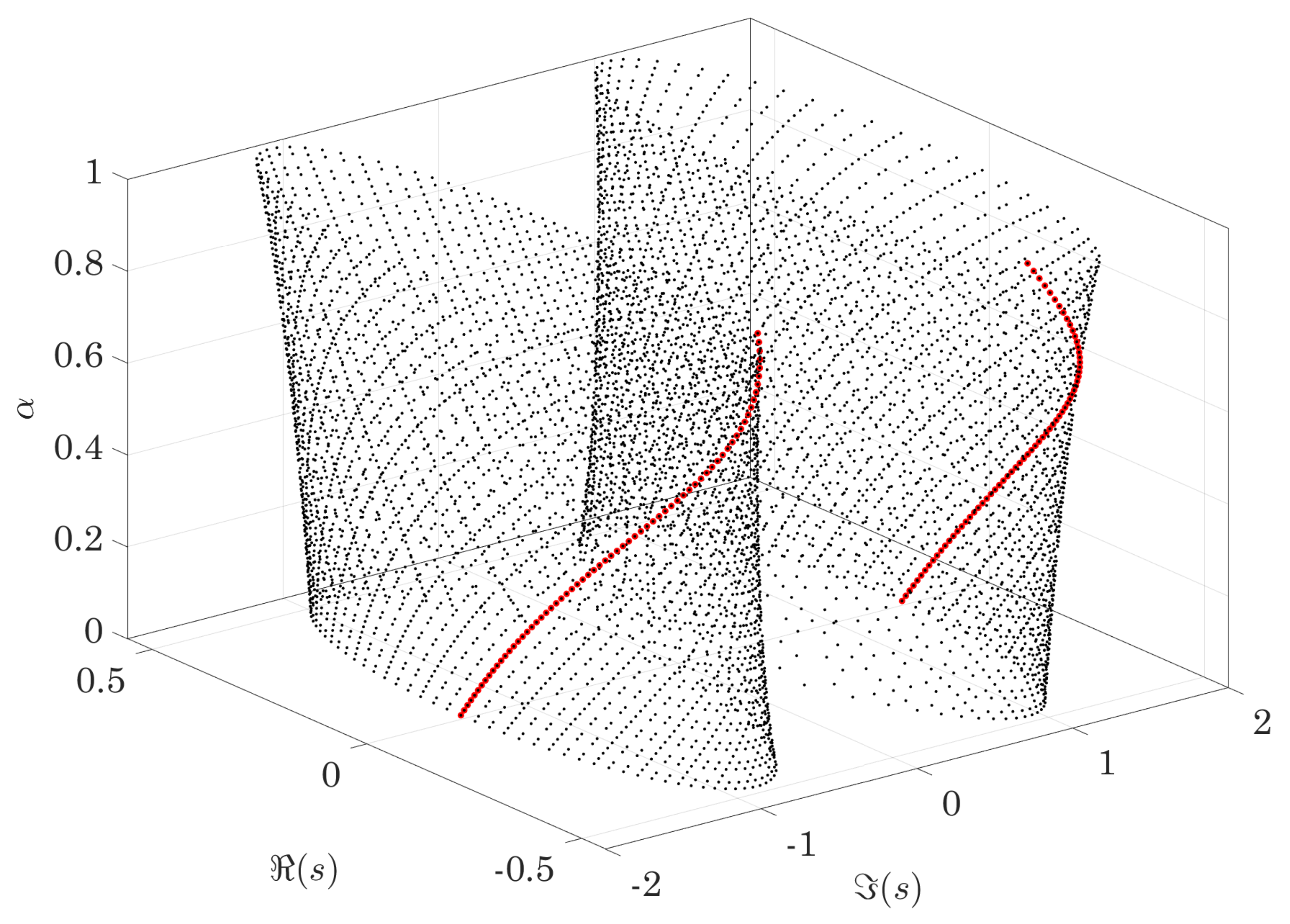
If the poles of the system for different values of $\alpha$ are plotted in the complex plane, the shape shown in Figure 1 is obtained. In it, the solutions obtained from the variable change in (6) are shown in black while the ones that satisfy (5) are highlighted in red.

For every value of $\alpha$, the centroid of each of the two distributions shown in Figure 1 computed as

$$C=\frac{1}{q}\sum _{j=1}^q{s}_j,$$

(7)

$s_j$ being the jth pole of the system and q the amount of solutions of (6) for each distribution, the extraneous ones included, fall in $\pm {\omega }_0=\pm \sqrt{k/m}$.

Another conclusion that can be drawn from the variation of the position of the poles with the value $\alpha$ is that, contrary to what could be expected, the number of decimal positions used to express $\alpha$ and, thus, the p and q values used to approximate it as a rational number, do not affect the position of the poles. This means that considering $\alpha$ or a slightly perturbed value $\alpha +\delta$ provides the same results both in terms of poles and, in consequence, of time response.

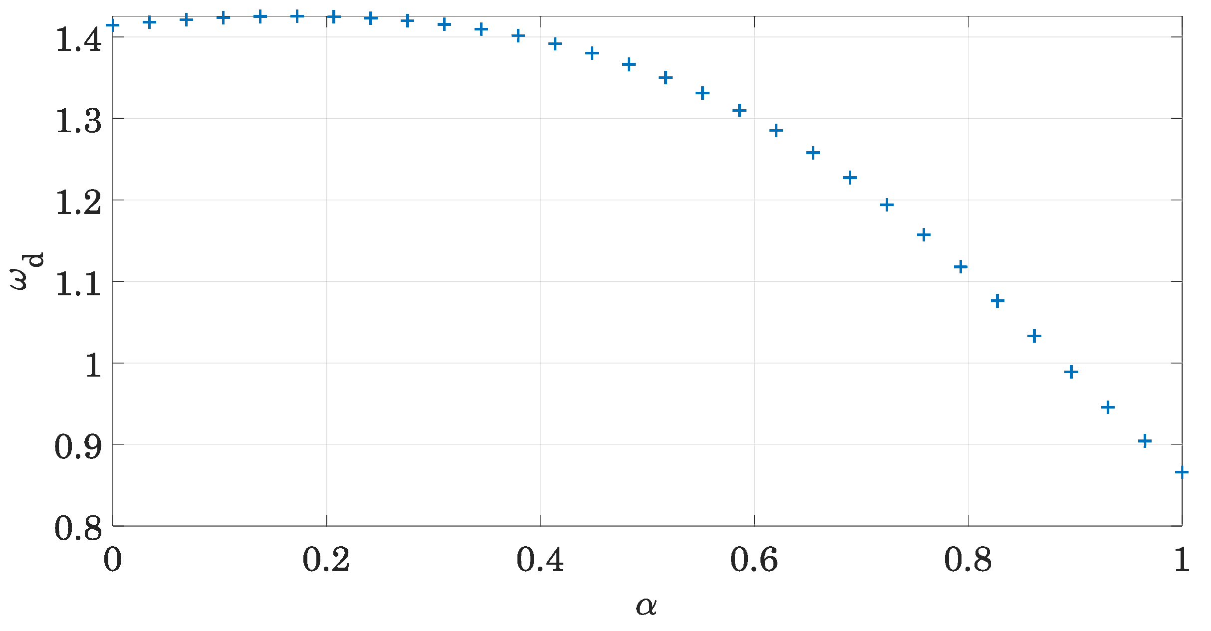
Then, the relationship of the damped frequency of the system, represented by the imaginary part of the poles, with the order of the derivative is studied. As shown in Figure 2, the damped frequency of the system ranges from

$${\omega }_{\mathrm{d}}=\sqrt{\frac{k+c}{m}}$$

(8)

when $\alpha$ = 0 (it should be noted that in this case, as the damper behaves like a spring, the system will be undamped) to the well known formula for the viscous case when $\alpha =1$

$${\omega }_{\mathrm{d}}={\omega }_0\sqrt{1-{\xi }^2},$$

(9)

where $\xi =c/\left(2\sqrt{km}\right)$ and ${\omega }_0=\sqrt{k/m}$. The damped frequency decays with the order of the derivative $\alpha$ because, due to the viscoelastic nature of the model, the lower this order, a bigger part of the damping behaves as stiffness [30].

Then, the value of the damping parameter c is changed keeping the order of the fractional derivative constant, in order to study the evolution of the damped frequency (Figure 3). In contrast to what happens in systems with viscous damping, increasing the damping parameter c in a fractionally damped system increases the vibration frequency. This can be explained again by the viscoelastic nature of fractional damping: while in a system with viscous damping a change in the value of the damping parameter c does not affect the stiffness; if the damping is fractional, both magnitudes are interrelated and an increase in the damping parameter c also stiffens the system. It is worth noting that, even if the tendency is the same for different values of the order of the derivative $\alpha$—increasing the damping parameter c produces an increase in the damped frequency—the relationship between the two magnitudes is not linear and varies depending on the value of the order of the derivative.

2.2. Dynamic Response

Another aspect in which a system with fractional damping differs from one showing viscous damping is the dynamic response. These differences are analysed in the 1 DOF system, first, when it is subjected to initial conditions and, after, when a impulse or step force is applied.

In order to make the analysis extensible to systems with several degrees of freedom or subjected to any type of excitation for which analytical solutions are not available, the process to solve the differential equation (1) numerically is presented. The analytical response of a 1 DOF system to the cited excitations—initial conditions or impulse and step forces—can be found, for instance, in [2,20,29,31].

That said, the Grünwald-Letnikov method is used to compute the values of the fractional derivative for a given time t. Its objective is to take advantage of the definition of the derivative and approximate the gamma functions with some recursively computed coefficients. The derivative of order $\alpha$ is, thus, expressed as

$${\mathrm{D}}^{\alpha }f\left(t\right)=\underset{\Delta t\to 0}{lim}\left(\frac{1}{{(\Delta t)}^{\alpha }}\sum _{j=0}^{S-1}\frac{\Gamma (j-\alpha )}{\Gamma (-\alpha )\Gamma (j+1)}f(t-j\Delta t)\right)$$

(10)

where $S=t/\Delta t$ is the number of samples. Considering

$$A_{j+1}=\frac{\Gamma (j-\alpha )}{\Gamma (-\alpha )\Gamma (j+1)},$$

(11)

the $A_j$ coefficients can be computed recursively by

$$\begin{array}{cc}\hfill A_1& =1,\hfill \end{array}$$

(12)

$$\begin{array}{cc}\hfill A_{j+1}& =\frac{j-\alpha -1}{j}{A}_j\hfill \end{array}$$

(13)

and the derivative of order $\alpha$ takes the simplified form

$${\mathrm{D}}^{\alpha }f\left(t\right)\approx \frac{1}{{(\Delta t)}^{\alpha }}\sum _{j=0}^{S-1}{A}_{j+1}f(t-j\Delta t),$$

(14)

which can be easily introduced in a numerical method, a forward Euler in this case.

It should be noted that fractional operators are convolution integrals and, as such, they have memory, making it is necessary to store the previous history so as to be able to compute the response in a certain step [1]. If needed, techniques as the one described in [30] could be used to reduce the storing requirements.

The presented methodology is followed in the next sections to compute the response of the fractionally damped 1 DOF system under study to initial conditions and to a impulse and step force, two of the most typical excitations.

2.2.1. Response to Initial Conditions

The response of a fractionally damping system whose m, c and k parameters are unitary and subjected to the initial conditions $\left\{x_0,v_0\right\}=\left\{1,0\right\}$ is shown in Figure 4. As predicted from the poles of the system, the response is oscillatory and decays in time.

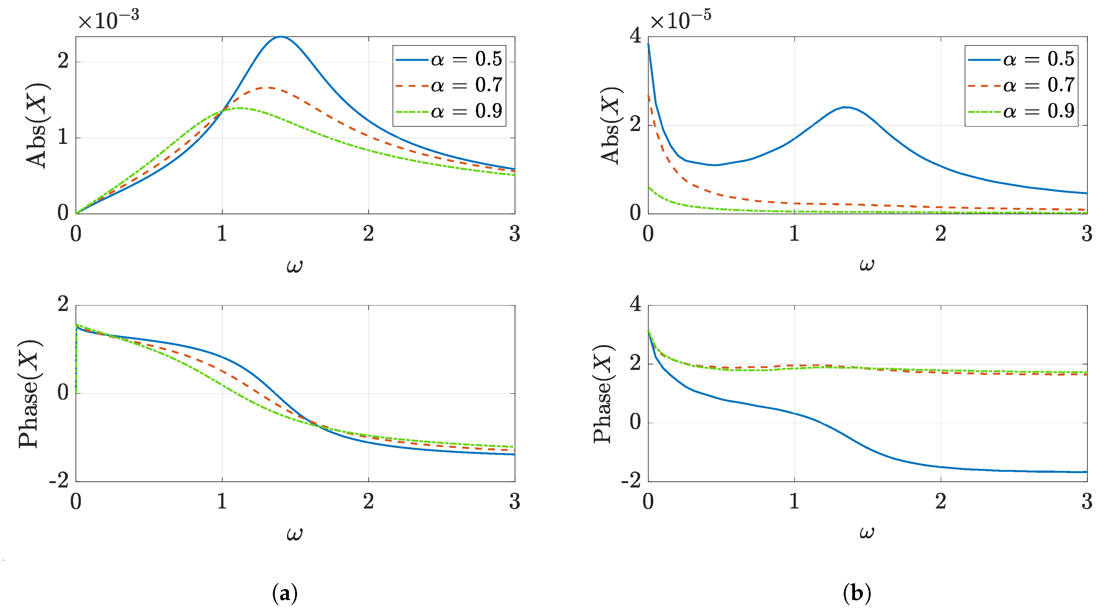
The main difference that a system with fractional damping presents in comparison to one that shows viscous damping regarding its response to initial conditions is the appearance of a non oscillatory term that decays in time [19]. This effect can be seen in Figure 5, where the response in the frequency domain, obtained by the Fast Fourier Transform of the time response, is represented for different values of the order of derivative $\alpha$. During the initial part of the response (Figure 5a), only a peak at the vibration frequency can be noticed; in the final part of the decay (Figure 5b), however, it is possible to identify also a peak in the spectrum at zero frequency, that is related to the non oscillatory term, together with the peak at the vibration frequency.

From a physical point of view, the appearance of a non oscillatory term has two implications. First, it means that the equilibrium position of the system is not constant but it varies with time. Taking into account that the equilibrium position is defined by the mass and the stiffness of the system and, in this case, the mass is constant, the single explanation to this phenomenon is that the stiffness of the system varies with time. Secondly, it implies that the system does not oscillate with decreasing amplitude until it finally stops, but that it reaches a point in which it approaches the original equilibrium position without oscillating.

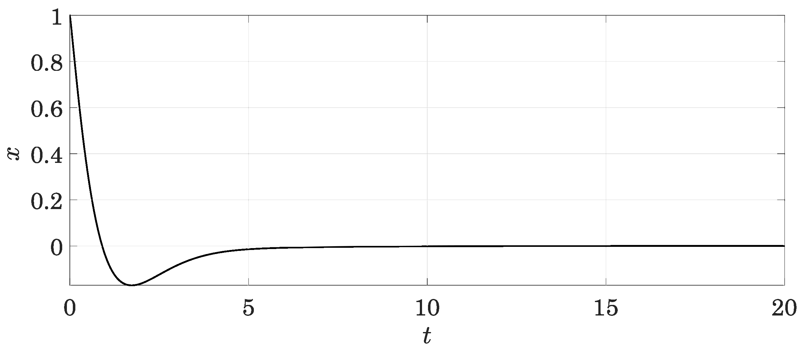
Another aspect in which a system with fractional damping differs from one with viscous damping is in the fact that a critical damping ratio in which the system does not oscillate around the equilibrium position cannot be defined [20,30]. The response always crosses the origin of coordinates at least once due to the nature of the poles of the system, that are always complex conjugates. For this reason, fractional damping allows us to model dampers whose response only crosses the equilibrium position a single time, a case that cannot be represented with accuracy using a traditional model. For example, the 1 DOF system under study presents this behaviour when the damping parameter $c=$ 2 and the order of the derivative $\alpha$ = 0.9 (Figure 6).

2.2.2. Response to Impulse

The response to an impulse is of interest because it provides a way to define critical damping. According to [20], critical damping can be defined for systems with fractional damping as the value for which the response is tangent to the axis of zero displacement when an impulse force

$$F\left(t\right)=\left\{\begin{array}{c}1/\Delta t,0<t<\Delta t\hfill \\ 0,\mathrm{otherwise}\hfill \end{array}\right.$$

(15)

is applied to the system. This means that for values of damping greater than this the response does not change sign, even if it still oscillates, around a position that varies with time in this case (Figure 7).

Following this reasoning, the value of critical damping can be estimated for different values of the order of the derivative $\alpha$. For example, in Figure 8, the response of the 1 DOF system with unitary mass and stiffness parameters and critical damping when subjected to a impulse is presented. For low values of $\alpha$ the response always changes sign no matter how high the added damping: increasing the damping parameter makes the system stiffer and the effect of the increase in the natural frequency is greater than that of the dissipation.

2.2.3. Response to Step

The response of the system with fractional damping to a step force

$$F\left(t\right)=\left\{\begin{array}{c}0,t<0\hfill \\ 1,0\le t\hfill \end{array}\right.$$

(16)

has the peculiarity that it stays under the response of a system with viscous damping. As an example, the response of the 1 DOF of freedom system with unitary mass, damping and stiffness constants under study is presented in Figure 9 depending of the order of the derivative $\alpha$ for a unit step excitation. It can be noted that for systems with fractional damping the overshoot decreases but the settling time is much longer, specially when decreasing the value of the order of the derivative.

3. Application: Bearing Support

In order to illustrate the properties of the fractional models presented in the previous sections in a real life application, a shaft supported by one bearing in each end is considered. The shaft is modelled by means of beam finite elements; both supports, following the typical model of a bearing [32], as a combination of a spring and fractional damper (Figure 10).

For the numerical application, a shaft of length $L=$ 1 m and circular section of diameter $d=$ 0.4 m made of steel with a Young’s modulus of $E=$ 210 GPa and density $\rho =$ 7900 kg/m³ is considered. The natural frequencies, mode shapes and response of the shaft when changing the parameters of the bearings are studied, the two bearings being identical ($k_1=k_{N-1}=k$, $c_1=c_{N-1}=c$ and ${\alpha }_1={\alpha }_{N-1}=\alpha$).

3.1. Natural Frequencies and Mode Shapes

The eigenpairs of a the shaft supported by bearings that present fractional damping satisfy the relationship

$$\left(-{\lambda }_r^{*}\mathbf{M}+{\mathbf{K}}_{\mathrm{shaft}}+{\mathbf{K}}_{\mathrm{supp}}^{*}\left({\omega }_r\right)\right){\mathsf{\varphi }}_r^{*}=\mathbf{0},$$

(17)

where ${\lambda }_r^{*}$ and ${\mathsf{\varphi }}_r^{*}$ are respectively the eigenvalue and the eigenvector of the rth mode, $\mathbf{M}$ the mass matrix of the system, that corresponds to the mass matrix of the shaft as the supports are considered massless, ${\mathbf{K}}_{\mathrm{shaft}}$ and ${\mathbf{K}}_{\mathrm{supp}}^{*}\left(\omega \right)$ the stiffness matrices of the shaft and the bearing supports. This last complex matrix ${\mathbf{K}}_{\mathrm{supp}}^{*}\left(\omega \right)$ is frequency dependent and is defined as

$${\mathbf{K}}_{\mathrm{supp}}^{*}\left(\omega \right)=\sum _{j\in B}(k_j+c_j{\left(\mathrm{i}\omega \right)}^{\alpha }){\mathbf{e}}_j{\mathbf{e}}_j^{⊺}/B=\{1,N-1\},$$

(18)

where B holds the positions of the bearing supports, in this case the first and penultimate (N − 1) degrees of freedoms, the ones that represent the vertical displacement of the first and last nodes, respectively and ${\mathbf{e}}_j$ stands for the unit vector that corresponds to the jth degree of freedom. As the matrix ${\mathbf{K}}_{\mathrm{supp}}$ is frequency dependent, an iterative method is needed to obtain the eigenpairs of the system: the reader can find the details in [33,34].

With the aim of studying the evolution of the vibration frequencies of the system with the order of the derivative $\alpha$, the values of the stiffness and damping parameters of the bearing supports are set to $k={10}^4$ N/m and $c=50$ N s^$\alpha$/m respectively. When the shaft is discretised with 60 beam elements in its length the results shown in Figure 11 are obtained. It can be observed that, as deduced for the 1 DOF system, changing the order of the derivative affects the stiffness of the supports and, thus, the vibration frequencies.

Another aspect that should be taken into account regarding the eigenpairs is that the modes are complex due to the non-proportionality of the damping. When the value of the damping parameter c is low this effect is barely noticeable so, for the sake of clarity, its value is increased to $c=$ 1000 N s^$\alpha$/m in the computation of the mode shapes presented in Figure 12. The phase of the mode shape in each point of the shaft is represented with the aim of bringing to light the complex nature of the modes: if the mode were normal, the phase would change abruptly from $-\pi$ to $\pi$ (or vice versa) in the nodal points, but it is not what occurs.

It should be noted also that the mode shapes are not affected by the order of the derivative $\alpha$ but the complex nature of the modes is more acute for high values of $\alpha$ as the effect of the damping is higher.

3.2. Dynamic Response

Next, the time response of the shaft to a perturbation from the base is computed following the procedure in [35] by means of a $\mathbf{M}$-$\mathbf{C}$-$\mathbf{K}$ Newmark method. The details of the implementation of such method can be found in [22], but, in short, it consists of expressing the equation of motion of the system in the instant $n+1$ as

$$\mathbf{M}{\ddot{\mathbf{u}}}_{n+1}+\mathbf{C}{\left({\mathrm{D}}^{\alpha }\mathbf{u}\right)}_{n+1}+\mathbf{K}{\mathbf{u}}_{n+1}={\mathbf{F}}_{n+1},$$

(19)

and introducing the notation

$$\mathbf{M}{\ddot{\mathbf{u}}}_{n+1}+\overline{\mathbf{C}}{\dot{\mathbf{u}}}_{n+1}+\mathbf{K}{\mathbf{u}}_{n+1}={\overline{\mathbf{F}}}_{n+1},$$

(20)

where

$$\overline{\mathbf{C}}={(\Delta t)}^{1-\alpha }\mathbf{C}$$

(21)

and

$${\overline{\mathbf{F}}}_{n+1}={\mathbf{F}}_{n+1}-\frac{1}{{(\Delta t)}^{\alpha }}\mathbf{C}\left[{\mathbf{u}}_n+\sum _{j=1}^n{A}_{j+1}{\mathbf{u}}_{n+1-j}\right]$$

(22)

in order to use the Grünwald-Letnikov definition of the fractional derivative in the computations. In the case under study the mass matrix $\mathbf{M}$ is that of the shaft; the stiffness matrix $\mathbf{K}$ is the sum of the one of the shaft and the one of the supports

$$\mathbf{K}={\mathbf{K}}_{\mathrm{shaft}}+{\mathbf{K}}_{\mathrm{supp}}$$

(23)

where

$${\mathbf{K}}_{\mathrm{supp}}=\sum _{j\in B}{k}_j{\mathbf{e}}_j{\mathbf{e}}_j^{⊺}/B=\{1,N-1\},$$

(24)

and the damping matrix $\mathbf{C}$ is given by the damping of the bearing supports as

$$\mathbf{C}=\sum _{j\in B}{c}_j{\mathbf{e}}_j{\mathbf{e}}_j^{⊺}/B=\{1,N-1\}.$$

(25)

The time response of the supported shaft to a seismic excitation is computed as follows: first, the static response to a displacement of the rightmost end is computed; then, it is introduced into the presented Newmark scheme as an initial deformation ${\mathbf{u}}_0$. Four distinct cases are studied:

• Case 1: a viscous case ($\alpha =$ 1) with low stiffness ($k_{\mathrm{ref}}={10}^4$ N/m) and low damping ($c_{\mathrm{ref}}=50$ N s/m) that is used for reference, in which the rigid body movement prevails.
• Case 2: a viscous case ($\alpha =$ 1) with low stiffness ($k=k_{\mathrm{ref}}$) and supercritical damping ($c=10c_{\mathrm{ref}}$), in which the shaft returns to the equilibrium position without oscillating.
• Case 3: a fractionally damped case ($\alpha =$ 0.6) with low stiffness ($k=k_{\mathrm{ref}}$) and high damping ($c=100c_{\mathrm{ref}}$) so that the system returns to its original position oscillating around a variable equilibrium position.
• Case 4: a fractionally damped case ($\alpha =$ 0.6) with high stiffness ($k=10k_{\mathrm{ref}}$) and low damping ($c=c_{\mathrm{ref}}$), in which the movement is a combination of the rigid body motion and the first modes of the system.

The four cases are simulated for a time $T=$ 1 s using 1000 samples and discretising the shaft with 60 beam elements. In order to analyse the difference between the cases, the displacement of the right end, to which a vertical displacement of 3 mm is imposed in the first instant, is plotted over time (Figure 13).

The first case represents the classical vibration damped in time: this behaviour can be modelled both with a viscous and a fractional damper. The motion of the second case, instead, is characteristic of a overdamped system and only achievable if the damping is viscous: a fractionally damped system will always oscillate, even if the response does not have to necessarily change sign, as the third case makes clear. Finally, the fourth case represents a more general situation in which the response consists of a combination of several modes and the rigid body motion. In this case, by tuning the stiffness and damping parameters and the order of the derivative, different behaviours can be reproduced.

The evolution of the shaft in time can be seen in the four videos provided as Supplementary Materials with this article.

4. Conclusions

This work discusses the behaviour of a 1 DOF system with fractional damping from the point of view of dynamics, specially focusing in the divergence of such a model of damping from a classical viscous one.

The first difference between a system with viscous and a fractional damping is that the poles of the latter are always complex conjugates, which implies that the response is always oscillatory and that, therefore, the concept of critical damping as defined for viscous systems is not applicable. Also, due to the viscoelastic nature of fractional damping, the damped frequency of the system decreases with the order of the derivative, as the system resembles more a pure viscous system, but increases with the damping parameter, as the contribution to the stiffness of the system increases too.

Several particularities can be observed regarding the time response as well. First, the response to initial conditions is characterised by the appearance of a non oscillatory term, which can be understood as a change in the position of the equilibrium position in time. Secondly, the response to an impulse allows us to define critical damping for this kind of systems as the amount of damping needed for the response not to change its sign. Finally, the response to a step function is characterised by its reduced overshoot but longer settling time is comparison to a system with viscous damping.

Despite their peculiarities, fractional models are useful to ease the modelling process and replicate behaviours that would otherwise require complex formulations. This is the case, for example, of the bearing support represented in this work with a spring and fractional damper for which behaviours that range from a traditional viscous case to an oscillating case with variable equilibrium position can be represented with a single model.

As a final remark, we would like to warn against using fractional models as mathematical artifacts that allow us to simplify the modelling process. It is advisable to check if the behaviour of the mechanical system under study follows the same trends as the assumed model, or at least, that the effects attributable to the model do not interfere in the computations.

References

- Adolfsson, K.; Enelund, M.; Olsson, P. On the fractional order model of viscoelasticity. Mech. Time Depend. Mater. 2005, 9, 15–34. [Google Scholar] [CrossRef]
- Podlubny, I. Fractional Differential Equations: An Introduction to Fractional Derivatives, Fractional Differential Equations, to Methods of Their Solution and Some of Their Spplications; Mathematics in Science and Engineering; Academic Press: Cambridge, MA, USA, 1999. [Google Scholar]
- Torvik, P.J.; Bagley, R.L. On the Appearance of the Fractional Derivative in the Behavior of Real Materials. J. Appl. Mech. 1984, 51, 294–298. [Google Scholar] [CrossRef]
- Bagley, R.L.; Torvik, P.J. A theoretical basis for the application of fractional calculus to viscoelasticity. J. Rheol. 1983, 27, 201–210. [Google Scholar] [CrossRef]
- Di Paola, M.; Pirrotta, A.; Valenza, A. Visco-elastic behavior through fractional calculus: An easier method for best fitting experimental results. Mech. Mater. 2011, 43, 799–806. [Google Scholar] [CrossRef] [Green Version]
- Nutting, P.G. A new general law of deformation. J. Frankl. Inst. 1921, 191, 679–685. [Google Scholar] [CrossRef]
- Gemant, A. A method of analyzing experimental results obtained from elasto-viscous bodies. Physics 1936, 7, 311–317. [Google Scholar] [CrossRef]
- Pinnola, F.P.; Zavarise, G.; Prete, A.D.; Franchi, R. On the appearance of fractional operators in non-linear stress–strain relation of metals. Int. J. Non-Linear Mech. 2018, 105, 1–8. [Google Scholar] [CrossRef] [Green Version]
- Makris, N. Three-dimensional constitutive viscoelastic laws with fractional order time derivatives. J. Rheol. 1997, 41, 1007–1020. [Google Scholar] [CrossRef]
- Alotta, G.; Barrera, O.; Cocks, A.C.; Di Paola, M. On the behavior of a three-dimensional fractional viscoelastic constitutive model. Meccanica 2017, 52, 2127–2142. [Google Scholar] [CrossRef] [Green Version]
- Alotta, G.; Barrera, O.; Cocks, A.; Paola, M.D. The finite element implementation of 3D fractional viscoelastic constitutive models. Finite Elem. Anal. Des. 2018, 146, 28–41. [Google Scholar] [CrossRef]
- Heymans, N.; Podlubny, I. Physical interpretation of initial conditions for fractional differential equations with Riemann-Liouville fractional derivatives. Rheol. Acta 2006, 45, 765–771. [Google Scholar] [CrossRef] [Green Version]
- Di Paola, M.; Pinnola, F.P.; Zingales, M. A discrete mechanical model of fractional hereditary materials. Meccanica 2013, 48, 1573–1586. [Google Scholar] [CrossRef] [Green Version]
- Schiessel, H.; Metzler, R.; Blumen, A.; Nonnenmacher, T.F. Generalized viscoelastic models: their fractional equations with solutions. J. Phys. Math. Gen. 1995, 28, 6567. [Google Scholar] [CrossRef]
- Naber, M. Linear fractionally damped oscillator. Int. J. Differ. Equations 2010, 2010. [Google Scholar] [CrossRef] [Green Version]
- Achar, B.N.N.; Hanneken, J.W.; Enck, T.; Clarke, T. Dynamics of the fractional oscillator. Phys. Stat. Mech. Appl. 2001, 297, 361–367. [Google Scholar] [CrossRef]
- Achar, B.N.N.; Hanneken, J.W.; Clarke, T. Response characteristics of a fractional oscillator. Phys. Stat. Mech. Appl. 2002, 309, 275–288. [Google Scholar] [CrossRef]
- Achar, B.N.N.; Hanneken, J.W.; Clarke, T. Damping characteristics of a fractional oscillator. Phys. Stat. Mech. Appl. 2004, 339, 311–319. [Google Scholar] [CrossRef]
- Shokooh, A.; Suárez, L. A comparison of numerical methods applied to a fractional model of damping materials. J. Vib. Control. 1999, 5, 331–354. [Google Scholar] [CrossRef]
- Suarez, L.E.; Shokooh, A. An eigenvector expansion method for the solution of motion containing fractional derivatives. J. Appl. Mech. 1997, 64, 629–635. [Google Scholar] [CrossRef]
- Fenander, A. Modal synthesis when modeling damping by use of fractional derivatives. AIAA J. 1996, 34, 1051–1058. [Google Scholar] [CrossRef]
- Cortés, F.; Elejabarrieta, M.J. Finite element formulations for transient dynamic analysis in structural systems with viscoelastic treatments containing fractional derivative models. Int. J. Numer. Methods Eng. 2007, 69, 2173–2195. [Google Scholar] [CrossRef]
- Cortés, F.; Elejabarrieta, M.J. Homogenised finite element for transient dynamic analysis of unconstrained layer damping beams involving fractional derivative models. Comput. Mech. 2007, 40, 313–324. [Google Scholar] [CrossRef]
- Mendiguren, J.; Cortés, F.; Galdos, L. A generalised fractional derivative model to represent elastoplastic behaviour of metals. Int. J. Mech. Sci. 2012, 65, 12–17. [Google Scholar] [CrossRef]
- Oldham, K.; Spanier, J. The Fractional Calculus Theory and Applications of Differentiation and Integration to Arbitrary Order; Elsevier: Amsterdam, The Netherlands, 1974. [Google Scholar]
- Hilfer, R. Applications of Fractional Calculus in Physics; World Scientific: Singapore, 2000. [Google Scholar]
- Miller, K.S.; Ross, B. An Introduction to the Fractional Calculus and Fractional Differential Equations; Wiley-Interscience: Hoboken, NJ, USA, 1993. [Google Scholar]
- Bagley, R.L.; Calico, R.A. Fractional order state equations for the control of viscoelasticallydamped structures. J. Guid. Control. Dyn. 1991, 14, 304–311. [Google Scholar] [CrossRef]
- Kilbas, A.A.A.; Srivastava, H.M.; Trujillo, J.J. Theory and Applications of Fractional Differential Equations; Elsevier Science Limited: Amsterdam, The Netherlands, 2006; Volume 204. [Google Scholar]
- Yuan, L.; Agrawal, O.P. A numerical scheme for dynamic systems containing fractional derivatives. Trans. Am. Soc. Mech. Eng. J. Vib. Acoust. 2002, 124, 321–324. [Google Scholar] [CrossRef] [Green Version]
- Pinnola, F.P. Statistical correlation of fractional oscillator response by complex spectral moments and state variable expansion. Commun. Nonlinear Sci. Numer. Simul. 2016, 39, 343–359. [Google Scholar] [CrossRef]
- Matsubara, M.; Rahnejat, H.; Gohar, R. Computational modelling of precision spindles supported by ball bearings. Int. J. Mach. Tools Manuf. 1988, 28, 429–442. [Google Scholar] [CrossRef]
- Cortés, F.; Elejabarrieta, M.J. Computational methods for complex eigenproblems in finite element analysis of structural systems with viscoelastic damping treatments. Comput. Methods Appl. Mech. Eng. 2006, 195, 6448–6462. [Google Scholar] [CrossRef]
- Cortés, F.; Elejabarrieta, M.J. An approximate numerical method for the complex eigenproblem in systems characterised by a structural damping matrix. J. Sound Vib. 2006, 296, 166–182. [Google Scholar] [CrossRef]
- Cortés, F.; Jesús Elejabarrieta, M. Finite element analysis of the seismic response of damped structural systems including fractional derivative models. J. Vib. Acoust. 2014, 136, 050901. [Google Scholar] [CrossRef]
Figure 1.
Distribution of poles for different values of . The solutions that comply with (5) are highlighted in red.
Figure 2.
Evolution of damped frequency with the order of the derivative . The mass, stiffness and damping parameters are unitary. The damped frequency ranges from to .
Figure 3.
Evolution of the damped frequency with the damping parameter c for different values of the order of the derivative .
Figure 4.
Time response of a fractionally damped system for different values of the order of the derivative.
Figure 5.
Response of a fractionally damped system in the frequency domain: (a) from t = 0 to t = 20, (b) for t > 20.
Figure 6.
Response of a single-degree-of-freedom (1 DOF) fractionally damped system with unitary mass and stiffness parameters, the order of the derivative being = 0.9 and the damping parameter 2 when subjected to initial conditions .
Figure 7.
Difference between an overdamped systems with viscous or fractional damping.
Figure 8.
Response to impulse of a system with critical damping for different values of the order of the derivative .
Figure 9.
Response to step for different values of .
Figure 10.
Shaft supported by a bearing in each end, where N stands for the number of degrees of freedom of the finite element model of the shaft. The bearing support affects the th degree of freedom, as the Nth is related to the rotation of the end.
Figure 11.
Evolution of the frequency of the first two modes with the order of the derivative .
Figure 12.
First five mode shapes of the supported shaft: real part and phase. The vibration frequencies of the mode shapes are the following: 116.20 rad/s, 320.24 rad/s, 1201.0 rad/s, 3144.6 rad/s and 6194.3 rad/s.
Figure 13.
Displacement of the right end of the shaft: (a) case 1, (b) case 2, (c) case 3, (d) case 4.
© 2019 by the authors. Licensee MDPI, Basel, Switzerland. This article is an open access article distributed under the terms and conditions of the Creative Commons Attribution (CC BY) license (http://creativecommons.org/licenses/by/4.0/).
Share and Cite
MDPI and ACS Style
Zarraga, O.; Sarría, I.; García-Barruetabeña, J.; Cortés, F. An Analysis of the Dynamical Behaviour of Systems with Fractional Damping for Mechanical Engineering Applications. Symmetry 2019, 11, 1499. https://doi.org/10.3390/sym11121499
AMA Style
Zarraga O, Sarría I, García-Barruetabeña J, Cortés F. An Analysis of the Dynamical Behaviour of Systems with Fractional Damping for Mechanical Engineering Applications. Symmetry. 2019; 11(12):1499. https://doi.org/10.3390/sym11121499
Chicago/Turabian StyleZarraga, Ondiz, Imanol Sarría, Jon García-Barruetabeña, and Fernando Cortés. 2019. "An Analysis of the Dynamical Behaviour of Systems with Fractional Damping for Mechanical Engineering Applications" Symmetry 11, no. 12: 1499. https://doi.org/10.3390/sym11121499
Note that from the first issue of 2016, this journal uses article numbers instead of page numbers. See further details here.