Hermite-Type Collocation Methods to Solve Volterra Integral Equations with Highly Oscillatory Bessel Kernels


1
College of Mathematics, Hunan Institute of Science and Technology, Yueyang 414006, China
2
College of Economics, Jinan University, Guangzhou 510632, China
3
School of Mathematics and Statistics, Central South University, Changsha 410083, China
*
Authors to whom correspondence should be addressed.
Symmetry 2019, 11(2), 168; https://doi.org/10.3390/sym11020168
Submission received: 20 December 2018
/
Revised: 21 January 2019
/
Accepted: 29 January 2019
/
Published: 1 February 2019
(This article belongs to the Special Issue Integral Transforms and Operational Calculus)
Abstract
:In this paper, we present two kinds of Hermite-type collocation methods for linear Volterra integral equations of the second kind with highly oscillatory Bessel kernels. One method is direct Hermite collocation method, which used direct two-points Hermite interpolation in the whole interval. The other one is piecewise Hermite collocation method, which used a two-points Hermite interpolation in each subinterval. These two methods can calculate the approximate value of function value and derivative value simultaneously. Both methods are constructed easily and implemented well by the fast computation of highly oscillatory integrals involving Bessel functions. Under some conditions, the asymptotic convergence order with respect to oscillatory factor of these two methods are established, which are higher than the existing results. Some numerical experiments are included to show efficiency of these two methods.
1. Introduction
Volterra integral equations arise from many mathematical problems in engineering and physics [1,2,3]. For example, the numerical solution of a scalar retarded potential integral equation posted on an infinite flat surface,
where u and a satisfy the causality condition , for all . The continuous Fourier transform (CFT) of a function is defined by . When for , by taking CFT, Davies and Duncan [2] reformulated it as the following Volterra integral equation of the first kind with highly oscillatory Bessel kernel,
where is the first-kind Bessel function of order m, which is the solution of the Bessel equation . In 2005, for the study of the problem of the electromagnetic scattering from a large cavity, G. Bao and W. W. Sun [1] reformulated (1) as a Volterra integral equation with Cauchy singular and highly oscillatory Hankel kernel.
The Bessel kernel of the above Equation (1) has a parameter . Obviously, when , the Bessel kernel function becomes highly oscillatory. When resort to numerical solutions of Equation (1), the computation of integrals involved Bessel kernel functions is inevitable. However, the classical quadrature rules, such as Newton-Cotes rule, Clenshaw-Curtis rule or Gauss rule, are failed to calculate this kind of integral. Hence, adopting suitable quadrature rules for the corresponding highly oscillatory integrals plays an important role in obtaining the numerical solution.
The function satisfies the condition of Theorem 2.1.8 ([4], p. 64). Upon differentiation with respect to x, the first-kind Volterra integral Equation (1) can be rewritten as the second-kind Volterra integral equations. In this paper, we treat the following Volterra integral equation of the second kind with highly oscillatory Bessel kernel
where is an unknown function, is a given smooth function, is the Bessel function of the first kind of order and the frequency is a parameter. When , the Bessel kernel function is highly oscillatory, and this makes solving Equation (2) a challenging problem.
In recent years, there has been tremendous interest in developing methods for solving highly oscillatory Volterra integral equation, such as discontinuous Galerkin method [5], Filon-type method [6,7], collocation method [4,8,9], collocation boundary value method [10,11], collocation method on uniform mesh [12], collocation method on graded mesh [13].
Xiang and Brunner [14] presented three methods: direct Filon method, piecewise constant collocation method and piecewise linear collocation method for the equation,
Based on the asymptotic analysis of the solution, they gave corresponding convergence rates in terms of the frequency for these methods. For the case of the , Fang et al. [15] showed that the optimal convergence with respect to the are respectively. These three methods, same as other existing methods, are constructed by original integral equation or its equivalent equation. Since only the function value in start point is used, which leads to low error precision. In this paper, we present two kinds of Hermite-type collocation methods by combining original integral equation and its differential equation. The new methods will use the values of function and derivative function in start point, which gets higher error precision than that of the above three methods.
The rest of the paper is organized as follows. In Section 2, we present two efficient methods for Equation (2): direct Hermite collocation method and piecewise Hermite collocation method. We show the error bound with respect to the frequency in Section 3. In Section 4, several numerical examples are included to verify the results of theoretical analysis. It is observed from numerical experiments that these methods have higher accuracy as compared with the Direct Filon method in [14].
2. Hermite-Type Collocation Methods
2.1. Direct Hermite Collocation Method (Algorithm 1)
Differentiate both sides of Equation (2),
Since
it follows that for the case ,
and for ,
Let us denote the Hermite interpolant polynomial between and by
where the polynomials
mean the fundamental polynomials with respect to the nodes 0 and . Then the collocation systems follow
where denotes an approximation of , denotes an approximation of . That is
Solving these systems, we get direct Hermite appromximate schemes for ,
for ,
where
denotes the moment
The specific calculation formula follows
The moments can be efficiently calculated by
where denotes the Gamma function and denotes the Lommel function of the second kind [16,17]. Once is large, the Lommel function can be efficiently approximated by truncating
| Algorithm 1: direct Hermite collocation method. |
| 1. Compute by (18); 2. Compute by (14)–(17); 3. Compute and by (13). |
2.2. Piecewise Hermite Collocation Method
To obtain higher-order approximations, a direct improvement of the direct Hermite collocation method is the composite Hermite collocation method, which is so-called piecewise Hermite collocation method (Algorithm 2), that is split the interval into several bins and apply the formula over each bin independently of the other.
Without loss of generality, suppose that is a uniform nodal point and is an approximation of such that is the Hermite interpolant polynomial between and for .
Let us define
where the polynomials
denote the fundamental polynomials with respect to the nodes and . Then the collocation systems follow
This leads to the piecewise Hermite collocation method
where
denotes the moment
The specific calculation formula is following that
| Algorithm 2: piecewise Hermite collocation method. |
| 1. Compute by (18); 2. Compute by (24); 3. Compute and by (22). |
3. Error Analyses
Firstly, we introduce some useful lemmas, which will be used to prove theorems for the later analyses.
Lemma 1
Lemma 2
([15], Lemma 2). Suppose and as Then for any and it is true that the integral
is uniformly bounded with respect to
Lemma 3
([18], Lemma 2.1). For any , and satisfies
- is integrable;
- and are bounded in for fixed respectively,
it is true that
where the constants and are independent of ω.
Let denote the linear Volterra integral operator defined by
and denote identity operator. Then Equation (2) can be reformulated more compactly as
To get the expression of (1)–(3) order derivatives of the solution of (2), we first discuss the relation between the integral operator and the differential operator D.
Theorem 1.
Assume . The Volterra operator defined by , where are the iterated kernels. Then the solution of (2) satisfies
where, and if Moreover, we have both of , and are uniformly bounded with respect to
Proof.
Let it follows that
Then
Since
this series is uniformly absolutely convergent, therefore we can differentiate it term by term
where if . □
If we define
and recall that , we find
Remark 1.
then, we have , and are uniform bounded with respect to .
Theorem 2.
Proof.
We only prove a situation . For the case , the proof method is similar.
By the definition of the direct Hermite collocation method, for any , it follows that
where be the error function. Interpolating E(x) at and , we have
where denotes the remainder of the Hermite interpolation. As we know satisfies that . Substituting (40) into (39), we are led to
That is
Therefore, the error can be computed by
where
Defining , then . From Lemma 1 to Lemma 3, we can easily get with respect to . What shall we do is prove that
Using integration by parts twice, we get
Denote
So, we only need to prove that
In the following, we show that the convergence degree of J with respect to .
Letting
then we have
Observing that
Notice that
where and are some constants independent of . For is cubic polynomial, we can easily show that with respect to According to Theorem 1 it follows that Together with Lemma 3 we can easily get
That is
Then
Therefore, we can get
□
Theorem 3.
Proof.
For the piecewise Hermite collocation method, satisfies
Combining the above equation with
we get
where and . An argument similar to the one used in Theorem 2 shows that
the desired result is then found by employing the generalized discrete Gronwall inequality ([4], p. 95). Similarly, one can derive the convergence order of . □
4. Numerical Examples
From Section 4, we can see that direct Hermite collocation method and piecewise Hermite collocation method are very efficient for solving the second-kind Volterra integral equation with highly oscillatory Bessel kernel. They possess the property that the higher oscillation, the higher accuracy. In this section, based on the Formulas (11), (13) and (22), we present some preliminary numerical experiments to verify the result of theoretical analysis. The experiments are performed on a 1.86 GHz PC with 2 GB of RAM. We are using the R2016a version of the Matlab system. The following Direct Filon method (DF) is presented in paper [14].
Example 1.
Consider the following equation
where . The analytic solution is .
In Table 1, we compare the relative error of from the DF method, piecewise linear collocation method, direct Hermite collocation, and piecewise Hermite collocation method. In Table 2, for fixed , we compare the relative error of from the piecewise linear collocation method and piecewise Hermite collocation method when the steps are different. In Figure 1, Figure 2 and Figure 3, we can see the convergence rate with respect to of these methods.
Example 2.
Consider the following equation,
where . The analytic solution is .
Example 3.
Consider the following equation,
where . The analytic solution is .
Example 4.
Consider the following equation,
where . The analytic solution is .
We can see the numerical solutions from the Figure 8.
From above examples, as can be seen, there is a good agreement between the present result and the exact solution. The Hermite-type collocation methods are better than DF method and PL collocation method. For Hermite-type collocation methods, the higher oscillation, the higher accuracy. For fixed frequency, the error is decrease with the increase of nodes.
5. Conclusions
Collocation methods are efficient in solving Volterra integral equation with highly oscillatory kernel. In this paper, we present two collocation methods: DH collocation method and piecewise Hermite collocation method. The first conclusion to be drawn from the numerical evidence presented earlier is that Hermite-type collocation methods are higher efficient than existent collocation methods. Both methods can calculate the approximate value of function value and derivative value simultaneously. Finally, while we have considered only the case of Bessel kernel in this paper, the Hermite-type collocation methods can be extended to Fourier kernel.
In the future work, we will study better methods to solve the Volterra integral equations with different kernel and Fredholm integral equations.
Author Contributions
C.F., G.H. and S.X. conceived and designed the experiments; C.F. performed the experiments; G.H. analyzed the data; C.F. contributed reagents/materials/analysis tools; C.F. and G.H. wrote the paper.
Funding
This work is supported partly by National Natural Science Foundation of China (No. 11701171, 11771454), the Scientific Research Fund of Hunan Provincial Education Department (No. 17B113 ), the Hunan Provincial Natural Science Foundation of China (No. 2016JJ4037), the Aid program for Science and Technology Innovative Research Team in Higher Educational Institutions of Hunan Province, the Fundamental Research Funds for the Central Universities (No. 21618333), and the Opening Project of Guangdong Province Key Laboratory of Computational Science at the Sun Yat-sen University (No. 2018010).
Acknowledgments
The authors are grateful to the anonymous referees for their useful comments and constructive suggestions for improvement of this paper.
Conflicts of Interest
The authors declare no conflict of interest.
References
- Bao, G.; Sun, W.W. A fast algorithm for the electromagnetic scattering from a large cavity. SIAM J. Sci. Comput. 2005, 27, 553–574. [Google Scholar] [CrossRef]
- Davis, P.J.; Duncan, D.B. Stability and convergence of collocation schemes for retarded potential integral equations. SIAM J. Numer. Anal. 2004, 42, 1167–1188. [Google Scholar] [CrossRef]
- Langdon, S.; Chandler-Wilde, S.N. A wavenumber independent boundary element method for an acoustic scattering problem. SIAM J. Numer. Anal. 2006, 43, 2450–2477. [Google Scholar] [CrossRef]
- Brunner, H. Collocation Methods for Volterra Integral and Related Functional Equations; Cambridge University Press: Cambridge, UK, 2004. [Google Scholar]
- Brunner, H.; Davis, P.J.; Duncan, D.B. Discontinuous Galerkin approximations for Volterra integral equations of the first kind. IMA J. Numer. Anal. 2009, 29, 856–881. [Google Scholar] [CrossRef]
- Ma, J.; Fang, C.; Xiang, S. Modified asymptotic orders of the direct Filon method for a class of Volterra integral equations. J. Comput. Appl. Math. 2015, 281, 120–125. [Google Scholar] [CrossRef]
- Wang, H.; Xiang, S. Asymptotic expansion and Filon-type methods for a Volterra integral equation with a highly oscillatory kernel. IMA J. Numer. Anal. 2011, 31, 469–490. [Google Scholar] [CrossRef]
- Brunner, H. On Volterra integral operators with highly oscillatory kernels. Discret. Contin. Dyn. Syst. 2014, 34, 915–929. [Google Scholar] [CrossRef]
- Ma, J.; Liu, H. On the Convolution Quadrature Rule for Integral Transforms with Oscillatory Bessel Kernels. Symmetry 2018, 10, 239. [Google Scholar] [CrossRef]
- Chen, H.; Zhang, C. Boundary value methods for Volterra integral and integro-differential equations. Appl. Math. Comp. 2011, 218, 2619–2630. [Google Scholar] [CrossRef]
- Ma, J.; Xiang, S. A Collocation Boundary Value Method for Linear Volterra Integral Equations. J. Sci. Comput. 2017, 71, 1–20. [Google Scholar] [CrossRef]
- Xiang, S.; Wu, Q. Numerical solutions to Volterra integral equations of the second kind with oscillatory trigonometric kernels. Appl. Math. Comp. 2013, 223, 34–44. [Google Scholar] [CrossRef]
- Wu, Q. On graded meshes for weakly singular Volterra integral equations with oscillatory trigonometric kernels. J. Comput. Appl. Math. 2014, 263, 370–376. [Google Scholar] [CrossRef]
- Xiang, S.; Brunner, H. Efficient methods for Volterra integral equations with highly oscillatory Bessel kernels. BIT Numer. Math. 2013, 53, 241–263. [Google Scholar] [CrossRef]
- Fang, C.; Ma, J.; Xiang, M. On Filon methods for a class of Volterra integral equations with highly oscillatory Bessel kernels. Appl. Math. Comp. 2015, 268, 783–792. [Google Scholar] [CrossRef]
- Watson, G.N. A Treatise on the Theory of Bessel Functions; Cambridge University Press: Cambridge, UK, 1952. [Google Scholar]
- Xiang, S.; Wang, H. Fast integration of highly oscillatory integrals with exotic oscillators. Math. Comp. 2010, 79, 829–844. [Google Scholar] [CrossRef]
- Ma, J.; Xiang, S.; Kang, H. on the convergence rates of Filon methods for the solution of a Volterra integral equation with a highly oscillatory Bessel kernel. Appl. Math. Lett. 2013, 26, 699–705. [Google Scholar] [CrossRef]
Sample Availability: Samples of the compounds …… are available from the authors. |
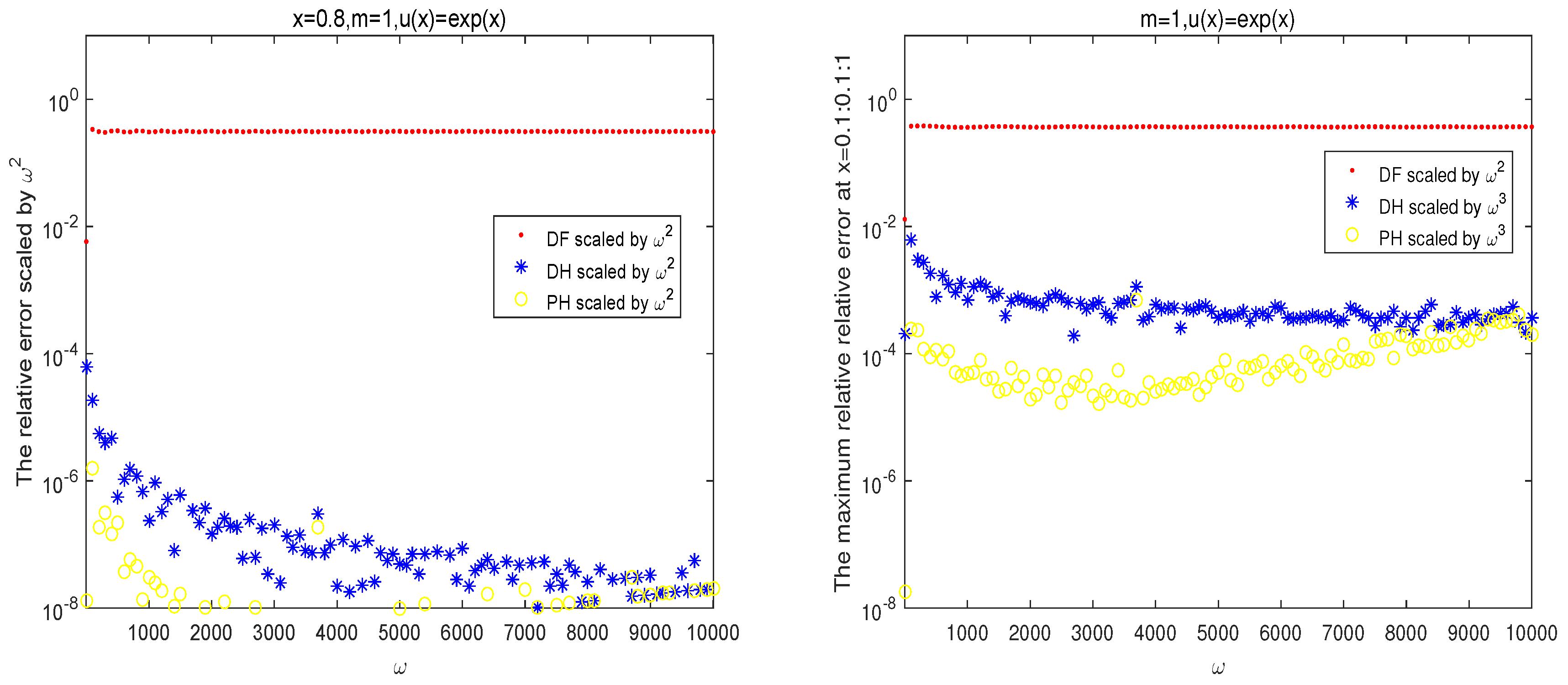
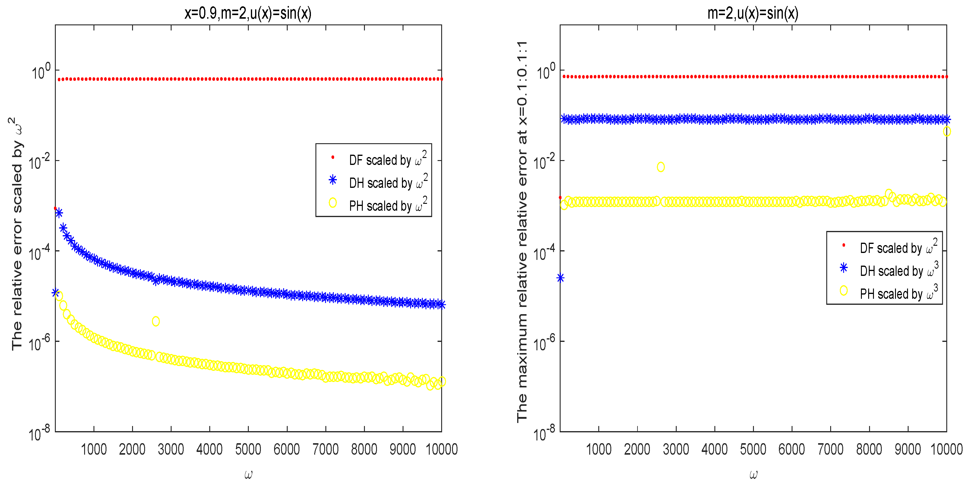
Figure 1.
The relative errors of for DF method, direct Hermite collocation method (DH) and piecewise Hermite collocation method (PH) at point (left), the maximum relative errors at collocation points x = 0.1:0.1:1 (right).
Figure 1.
The relative errors of for DF method, direct Hermite collocation method (DH) and piecewise Hermite collocation method (PH) at point (left), the maximum relative errors at collocation points x = 0.1:0.1:1 (right).

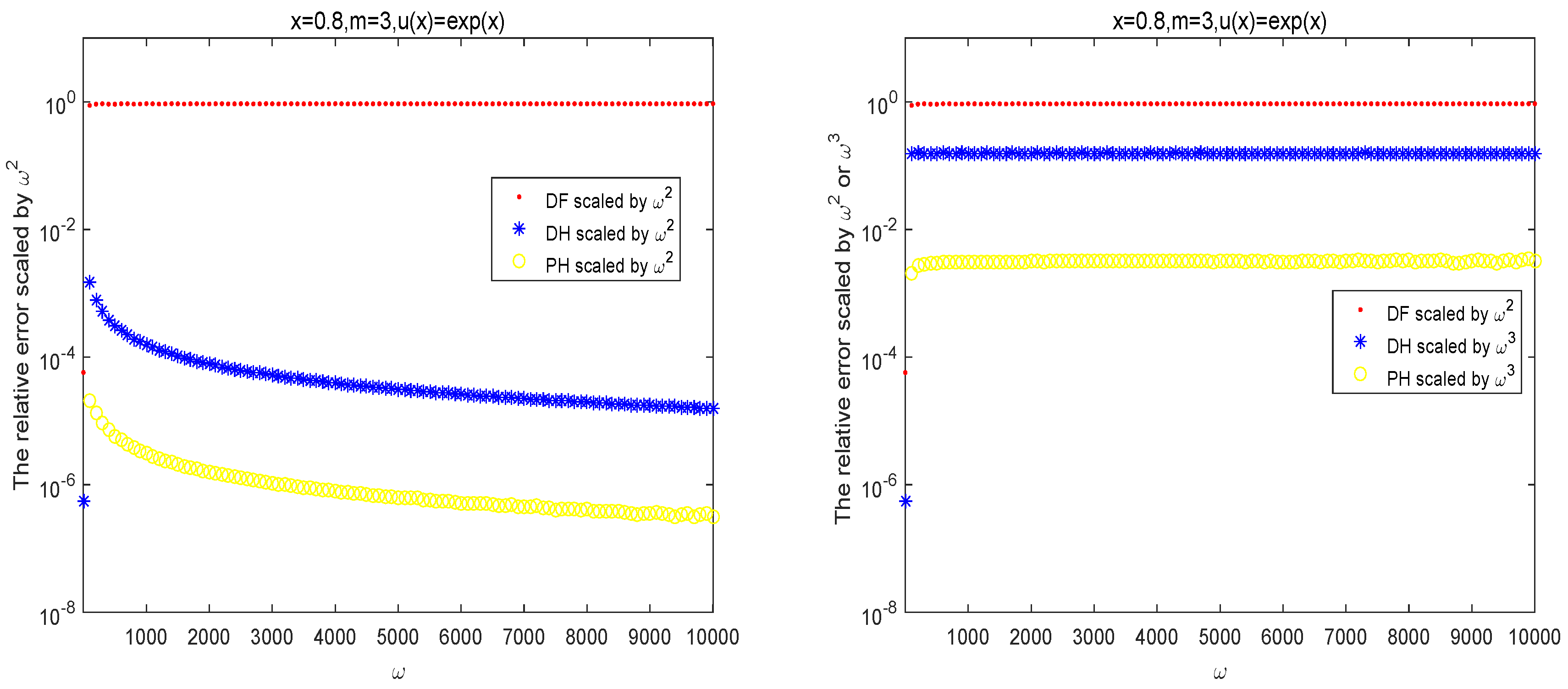
Figure 2.
The relative errors of at point for DF method, direct Hermite collocation method (DH), piecewise Hermite collocation method (PH).
Figure 2.
The relative errors of at point for DF method, direct Hermite collocation method (DH), piecewise Hermite collocation method (PH).

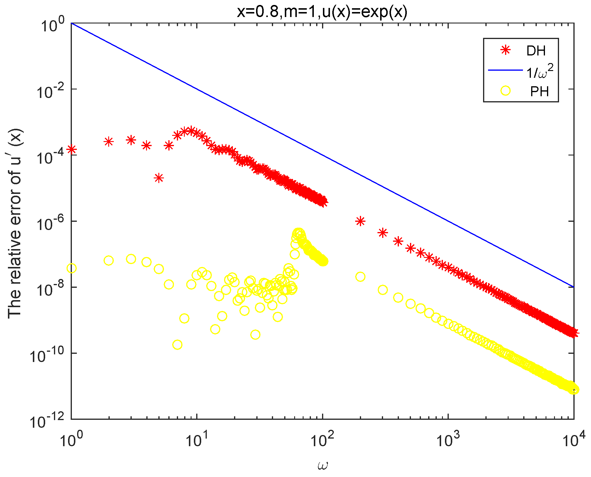
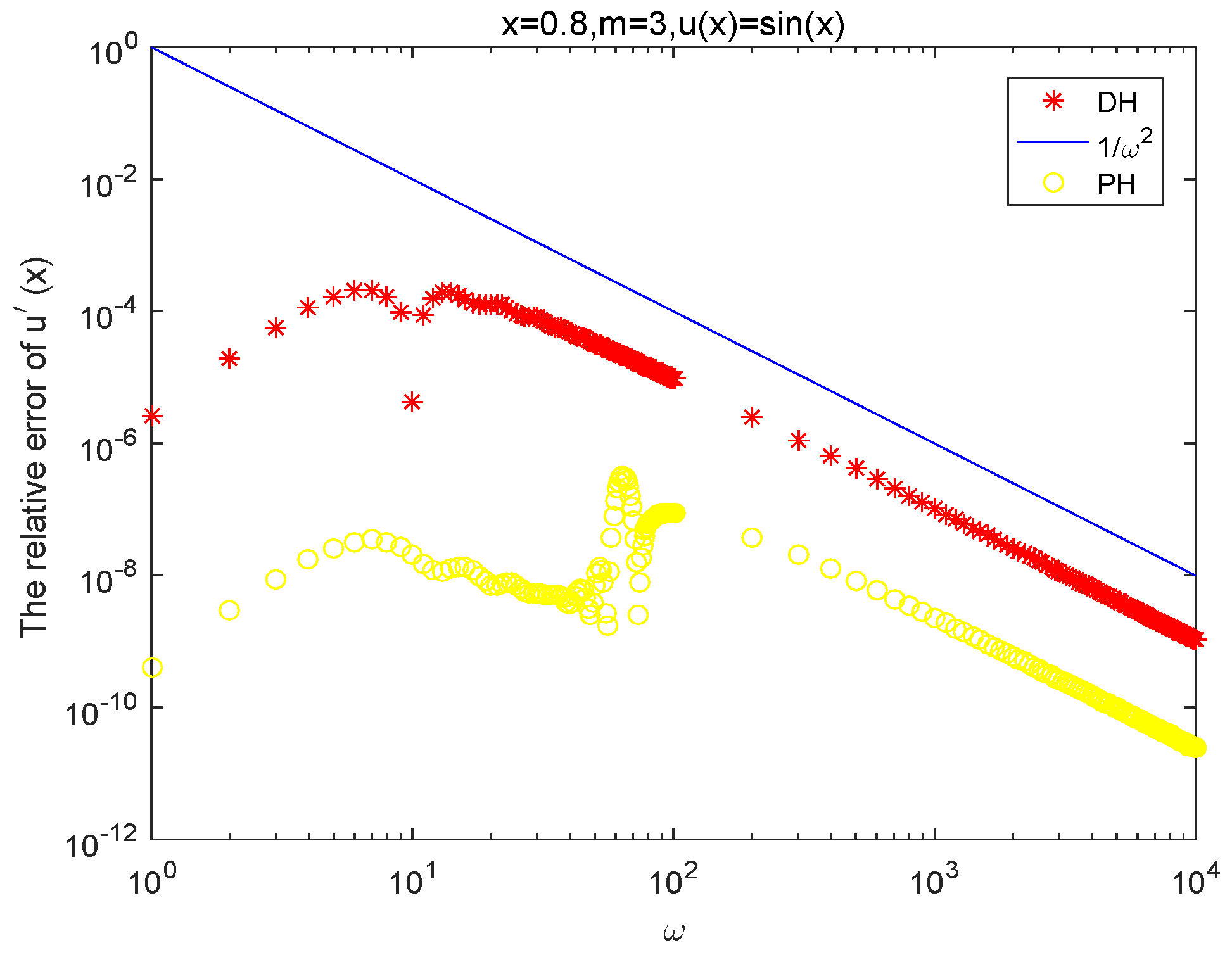
Figure 3.
The relative error of .

Figure 4.
The relative errors of for DF method, direct Hermite collocation method (DH) and piecewise Hermite collocation method (PH) at point (left), the maximum relative errors at collocation points x = 0.1:0.1:1 (right).
Figure 4.
The relative errors of for DF method, direct Hermite collocation method (DH) and piecewise Hermite collocation method (PH) at point (left), the maximum relative errors at collocation points x = 0.1:0.1:1 (right).

Figure 5.
The relative error of .

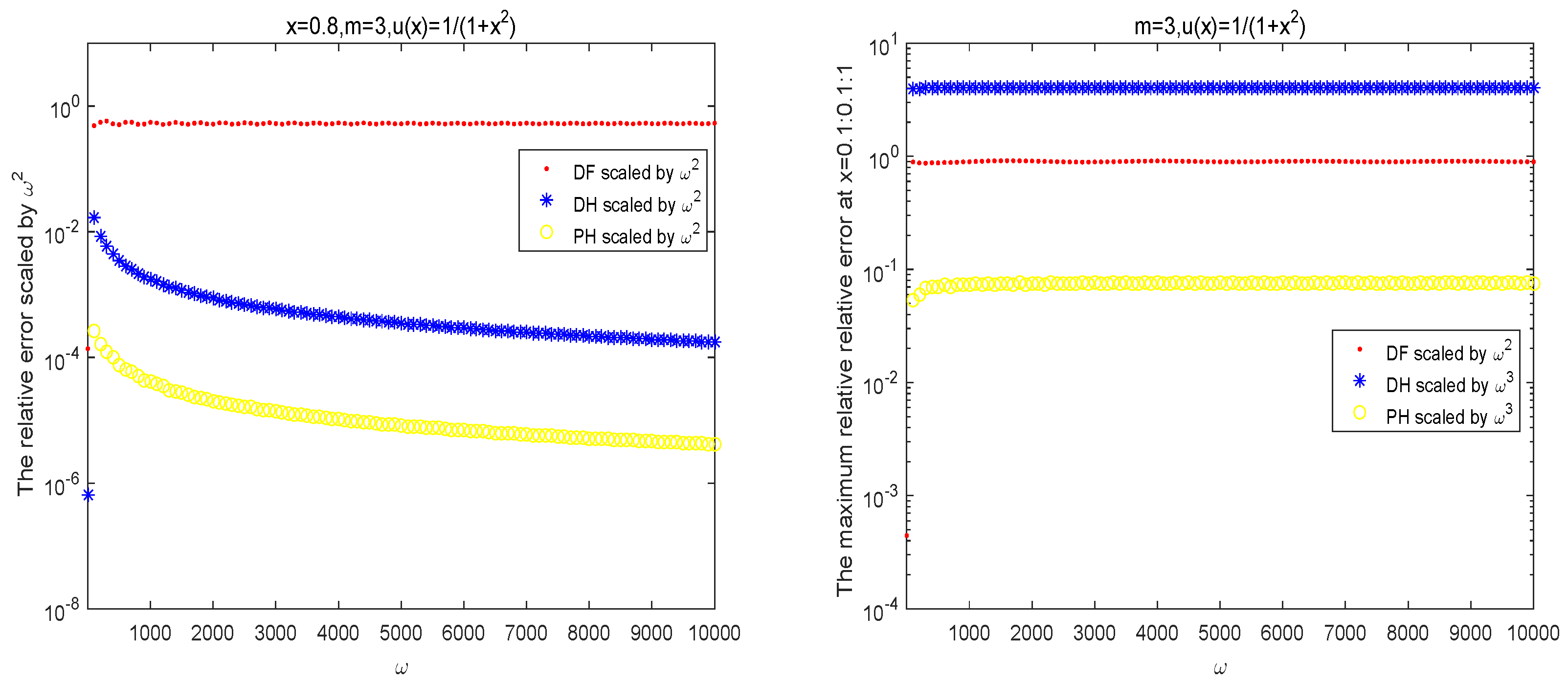
Figure 6.
The relative errors of for DF method, direct Hermite collocation method (DH) and piecewise Hermite collocation method (PH) at point (left), the maximum relative errors at collocation points x = 0.1:0.1:1 (right).
Figure 6.
The relative errors of for DF method, direct Hermite collocation method (DH) and piecewise Hermite collocation method (PH) at point (left), the maximum relative errors at collocation points x = 0.1:0.1:1 (right).

Figure 7.
The relative error of .

Figure 8.
The relative errors of and for direct Hermite collocation method (DH) and piecewise Hermite collocation method (PH).
Figure 8.
The relative errors of and for direct Hermite collocation method (DH) and piecewise Hermite collocation method (PH).


Table 1.
Relative errors of in N–point approximations to the Example 1 by the DF method, the piecewise linear method (PL), the direct Hermite method(DH) and the piecewise Hermite collocation method(PH). The step is 0.1 for piecewise method and the test point is 0.8.
Table 1.
Relative errors of in N–point approximations to the Example 1 by the DF method, the piecewise linear method (PL), the direct Hermite method(DH) and the piecewise Hermite collocation method(PH). The step is 0.1 for piecewise method and the test point is 0.8.
| 10 | ||||
| 100 | ||||
| 1000 | ||||
Table 2.
Relative errors of in N–point approximations to the Example 1 by the PL method and the piecewise Hermite collocation method(PH). where and the test point is 0.8.
Table 2.
Relative errors of in N–point approximations to the Example 1 by the PL method and the piecewise Hermite collocation method(PH). where and the test point is 0.8.
Table 3.
Relative errors of in N–point approximations to the Example 2 by the DF method, the PL method, the DH method, and the piecewise Hermite collocation method (PH). The step is 0.1 for piecewise method and the test point is 0.8.
Table 3.
Relative errors of in N–point approximations to the Example 2 by the DF method, the PL method, the DH method, and the piecewise Hermite collocation method (PH). The step is 0.1 for piecewise method and the test point is 0.8.
| 10 | ||||
| 100 | ||||
| 1000 | ||||
Table 4.
Relative errors of in N–point approximations to the Example 2 by the PL method and the piecewise Hermite collocation method (PH). where and the test point is 0.8.
Table 4.
Relative errors of in N–point approximations to the Example 2 by the PL method and the piecewise Hermite collocation method (PH). where and the test point is 0.8.
| 0 |
Table 5.
Relative errors of in N–point approximations to the Example 3 by the DF method and the PL method and the DH method, and the piecewise Hermite collocation method (PH). The step is 0.1 for piecewise method and the test point is 0.9.
Table 5.
Relative errors of in N–point approximations to the Example 3 by the DF method and the PL method and the DH method, and the piecewise Hermite collocation method (PH). The step is 0.1 for piecewise method and the test point is 0.9.
| 10 | ||||
| 100 | ||||
| 1000 | ||||
© 2019 by the authors. Licensee MDPI, Basel, Switzerland. This article is an open access article distributed under the terms and conditions of the Creative Commons Attribution (CC BY) license (http://creativecommons.org/licenses/by/4.0/).
Share and Cite
MDPI and ACS Style
Fang, C.; He, G.; Xiang, S. Hermite-Type Collocation Methods to Solve Volterra Integral Equations with Highly Oscillatory Bessel Kernels. Symmetry 2019, 11, 168. https://doi.org/10.3390/sym11020168
AMA Style
Fang C, He G, Xiang S. Hermite-Type Collocation Methods to Solve Volterra Integral Equations with Highly Oscillatory Bessel Kernels. Symmetry. 2019; 11(2):168. https://doi.org/10.3390/sym11020168
Chicago/Turabian StyleFang, Chunhua, Guo He, and Shuhuang Xiang. 2019. "Hermite-Type Collocation Methods to Solve Volterra Integral Equations with Highly Oscillatory Bessel Kernels" Symmetry 11, no. 2: 168. https://doi.org/10.3390/sym11020168
Note that from the first issue of 2016, this journal uses article numbers instead of page numbers. See further details here.