Identification-Method Research for Open-Source Software Ecosystems


1
School of Software, Central South University, Changsha 410075, China
2
Department of Information Management, Hunan University of Finance and Economics, Changsha 410075, China
3
Department of Computing, School of Computing, Engineering and Built Environment, Glasgow Caledonian University, Glasgow G4 0BA, UK
4
Department of Computer Science, Missouri State University, Springfield, MO 65897, USA
*
Author to whom correspondence should be addressed.
Symmetry 2019, 11(2), 182; https://doi.org/10.3390/sym11020182
Submission received: 26 December 2018
/
Revised: 30 January 2019
/
Accepted: 31 January 2019
/
Published: 3 February 2019
Abstract
:In recent years, open-source software (OSS) development has grown, with many developers around the world working on different OSS projects. A variety of open-source software ecosystems have emerged, for instance, GitHub, StackOverflow, and SourceForge. One of the most typical social-programming and code-hosting sites, GitHub, has amassed numerous open-source-software projects and developers in the same virtual collaboration platform. Since GitHub itself is a large open-source community, it hosts a collection of software projects that are developed together and coevolve. The great challenge here is how to identify the relationship between these projects, i.e., project relevance. Software-ecosystem identification is the basis of other studies in the ecosystem. Therefore, how to extract useful information in GitHub and identify software ecosystems is particularly important, and it is also a research area in symmetry. In this paper, a Topic-based Project Knowledge Metrics Framework (TPKMF) is proposed. By collecting the multisource dataset of an open-source ecosystem, project-relevance analysis of the open-source software is carried out on the basis of software-ecosystem identification. Then, we used our Spectral Clustering algorithm based on Core Project (CP-SC) to identify software-ecosystem projects and further identify software ecosystems. We verified that most software ecosystems usually contain a core software project, and most other projects are associated with it. Furthermore, we analyzed the characteristics of the ecosystem, and we also found that interactive information has greater impact on project relevance. Finally, we summarize the Topic-based Project Knowledge Metrics Framework.
1. Introduction
Since the late twentieth century, open-source software has made remarkable achievements. The focus of open-source-software research in academic and business circles is not only on open-source-software products, but also on open-source-software ecosystems [1]. There is a kind of social-coding site where developers gather in the same virtual environment, such as GitHub and SourceForge. Thus, a rapidly evolving phenomenon has emerged, software ecosystems. A software ecosystem is defined as a collection of software projects that are developed together and coevolve, due to project relevance and shared developer communities, in the same environment [2,3]. The ecosystem research area includes architecture, identification, evolution, and health. However, software systems are seldom developed in isolation; instead, they are developed with other projects in the wider context of an organization [2]. Most ecosystems revolve around one central project, illustrated by the case of GitHub. GitHub, a typical software ecosystem, owns the world’s largest collection of open-source-software projects, with around 24 million users across 200 countries and 67 million repositories up to 2017. Thus, analysis of software-ecosystem projects has emerged as a novel research area in recent years.
Software-ecosystem identification is the basis of other studies on ecosystems. The structure of an ecosystem can be well-defined by project relevance [4]. Thus, analysing project relevance is an effective way to identify ecosystems. Project relevance refers to interdependencies between projects due to developers’ behaviors. Research on project relevance can help developers improve the efficiency of collaborative development. Based on project relevance, we can further analyze project characteristics in the ecosystem that can be measured, for example, by project description, project language, project framework, and the number of project forks and stars. However, analysing project relevance at the ecosystem level can be challenging, and it has largely proven to be difficult. For instance, Ossher et al. [5] mentioned that it is simply not feasible to manually resolve interdependencies for thousands of projects, and many forms of analysis require declarative completeness. Existing static-relevance analysis methods do not identify interdependencies across projects. Methods for extracting relevance from a project’s source code have been proposed [5,6], but they require large amounts of memory and computation time [7]. Thus, they cannot be employed across a large set of projects. Other methods [2,8,9,10] avoid analyzing the source code by obtaining project-relevance information from a project’s configuration files, but this information is not always available or accurate. There is direct or indirect project relevance belonging to the same software ecosystem. In the past, when studying the software ecosystem of a single project, project relevance could be directly extracted from code or configuration, because the research scope was small and limited, while the scale and data volume of the open-source community are very large, and direct extraction is not feasible. A recent method for analysing project relevance, Reference Coupling [11], identifies user-specified links between the projects in the comments and has achieved good results, but these specified links may be hard to find or out of date.
To identify project relevance, we propose a Topic-based Project Knowledge Metrics Framework (TPKMF) based on GitHub-hosted projects. Our main task for software-ecosystem identification is to mine a subset of projects that belong to the same software ecosystem with similar attributes from the set of projects. In this paper, we used the TPKMF to construct the project-relevance network. We first collected the multisource data of the projects, including project information and interactive information. After a series of data preprocessing, we then analyzed the relevance of these projects’ data using our TPKMF. We confirmed that there were good interdependencies between the projects. We also used our Core Project–Spectral Clustering (CP-SC) algorithm to divide the project-relevance network. Finally, the impact of project information and interactive information on project relevance was explored. Our analysis was guided by the following research questions (RQs):
- How can a topic-based project knowledge metrics framework be leveraged to explore project relevance in project information and interactive information?
- Which ecosystems exist in the project-relevance network and what are their features?
- Which from project information and interactive information has a larger impact on project relevance?
The remaining parts of the paper are organized as follows: Our research methods and results are presented in Section 2 for RQ1, Section 3 for RQ2, and Section 4 for RQ3. In Section 5, we summarize our method and discuss problems. Section 6 presents an overview of related work on software ecosystems, project relevance, and social networks. We provide a brief conclusion and future work in Section 7.
2. Topic-Based Project Knowledge Metrics Framework
RQ1: How can topic-based project knowledge metrics framework be leveraged to explore project relevance in project information and interactive information?
2.1. Research Method
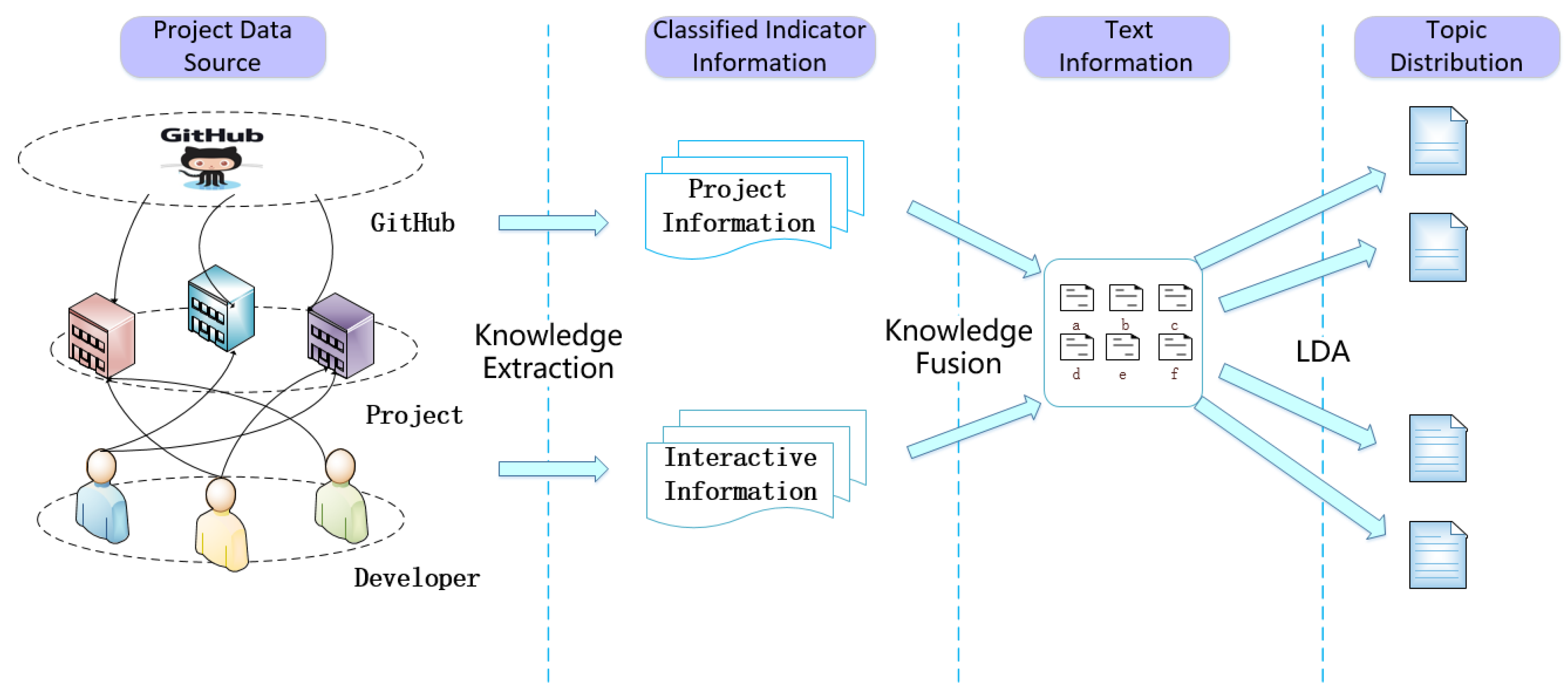
We analyzed project relevance in project information and interactive information by using the TPKMF. The framework can be summarized as three steps: First, extracting the corresponding data according to the GitHub-hosted projects and the behaviors of developers, and classifying them as project information and interactive information. Then, fusion of project information and interactive information, and constructing the topic–project relation matrix by LDA. Finally, constructing a similarity matrix and project-relevance network through the relation matrix. These steps are shown in Figure 1. We describe it in more detail in the following subsections.
2.1.1. Datasets
There are two main ways through which we can obtain data. Writing a web crawler program to obtain project information, as the GitHub project home page has a large number of project names, descriptions, file lists, discussion data, attention data, and other information. We define this information as project information. The other way is to obtain data from the GHTorrent project. These projects collect and update data for open-source ecosystems in real time, so we can directly obtain a dataset from these open-source data-collection projects, such as the GitHub mirror dataset provided by the GHTorrent project, and the GitHub event dataset provided by the GitHub Archive project. We selected six attributes of event data, pushEvent, pullrequestEvent, issuesEvent, commitCommentEvent, issueCommentEvent, and pullrequestReviewCommentEvent, and extracted their corresponding fields (message or body field). We define this information as interactive information.
After obtaining two major metrics of information, we preprocessed data through data cleaning and semantic analysis. We removed common English language stop words (such as ‘the’, ‘it’, and ‘on’) to reduce noise by the stop-word list provided by Google. In addition, we stemmed the words (for example, ‘fixing’ becomes ‘fix’) in order to reduce vocabulary size and reduce duplication due to word forms. Finally, the fusion of project information and interactive information was completed. We refer to them collectively as project-text data.
2.1.2. Structure of Relation Matrix
Based on the collected project-text data, we constructed the topic-project relation matrix by LDA, and set 10 as the best number of topics through much experimentation. Thus, we calculated the topic distribution and obtained the relation matrix. Each row represents a project, each column represents a topic, and values represent topic-distribution probability. Currently, the most popular topic models are PLSA and LDA [12]. LDA is an upgraded version of PLSA, which introduced Dirichlet prior distribution. PLSA is more suitable for short text, while LDA is more suitable for long text. Since project-text data include title, descriptions, and comments, it may be more suitable to be classified as long text. Hence, we adopted the LDA as the topic model to construct the relation matrix.
2.1.3. Similarity-Matrix Construction
Because the construction of a similarity matrix is the foundation of network construction, we calculated the similarity of two texts, which can be achieved by calculating topic distribution. We calculated text similarity by using the JS distance converted from the KL distance to obtain the similarity matrix, so that
where p and q are representative of the topic distribution between the projects. The similarity matrix is based on JS distance, since 0–1 is JS distance, and we set a threshold of 0.8 through many experiments; if distance between the projects were greater than 0.8, we set the dependent weights between the projects to 1, and the rest to 0, after converting the similarity matrix into a 0–1 matrix. Then, we set the values of the diagonals to 0 in order to facilitate the construction of the network.
2.2. Result
For the similarity matrix, we constructed an undirected network graph G = < V, E >. The project-relevance network can be denoted by G. The project node can be denoted by V. The edge weight, denoted by E, is 1. We filtered the edges if the the distance between the projects was smaller than 0.8 to capture only the stronger interdependencies.
We use the topic-based project knowledge metrics framework to identify project relevance and then build a 10,133-project relevance network, as shown in Figure 2. This stands for a project-relevance network with a degree of at least 1, 2, and 3. The network of Figure 2a shows weak relevance and, although the network of Figure 2c shows the strongest relevance, it is very sparse. We therefore filtered the edges to only consider interdependencies between nodes if the pair of projects was connected twice or more times to only capture the stronger and denser interdependencies.
Of the 10,133 projects in the Relevance Network, 2330 (23%) were a part of the largest connected component (commonly referred to as the giant component), which is the largest subgraph through which every node is connected to every other node by a path. The connected components isolated from the giant component are primarily comprised of same owner communities in which all nodes in the connected component are projects owned by the same GitHub developer or organization. For instance, the second-largest connected component consists of 229 nodes, all of which are owned by GitHub developer deathcap except for two nodes. Figure 2b shows the full relevance network, though for visibility we only display nodes with total weight of 2 or greater. As can be seen on the graph, most of the nodes isolated from the giant component are only connected to a small number of nodes.
3. Spectral-Clustering Algorithm Based on Core Project for Ecosystem Identification
RQ2: Which ecosystems exist in the project-related network and what are their features?
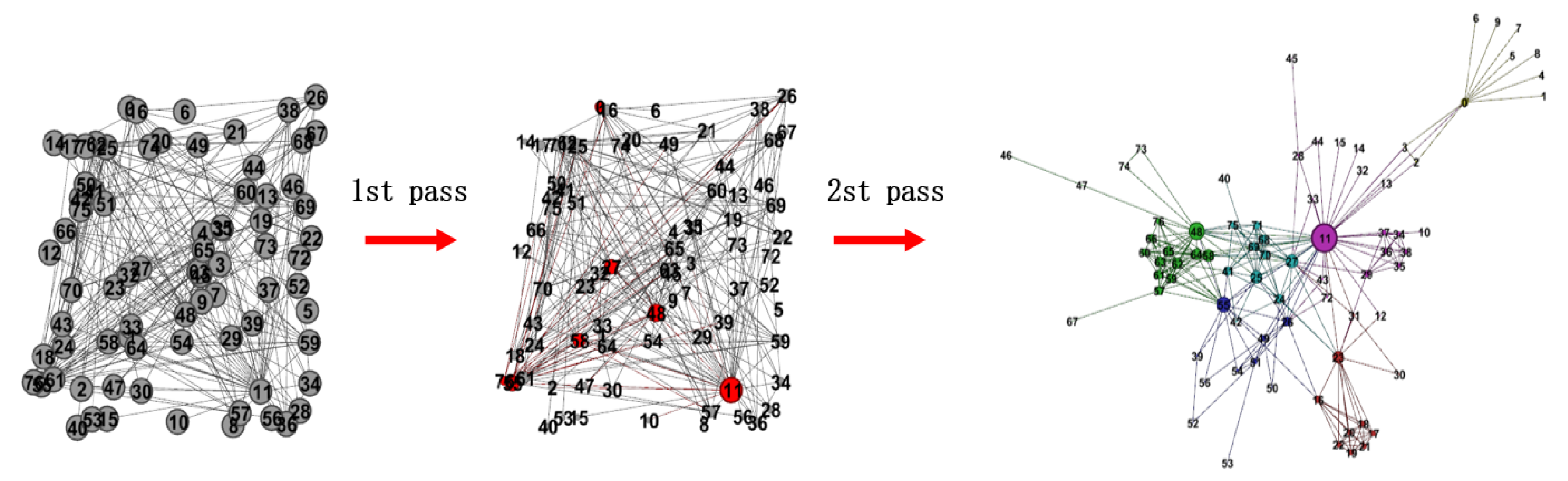
We constructed a network of the project-relevance relationships established through TPKMF as described in Section 2. To identify ecosystems, we needed to divide the project-relevance network. Software ecosystems usually contain a core project, and other projects in the ecosystem depend on core projects or are closely related to them. Core projects usually have greater influence on open-source communities. To this end, this section proposes a Spectral Clustering algorithm based on the Core Project (CP–SC) for ecosystem identification in the project-relevance network. The idea of the algorithm is to calculate the conductance of all nodes in the network, select the initial clustering center nodes, which are smaller, and disperse them as much as possible, and then run the k-means algorithm on spectral-clustering division vector , and obtain the community division results. The overview of CP–SC is shown in Figure 3. We describe it in more detail in the following subsections.
3.1. Related Definition
Given set of vertices V, set M is the subset of V, set is the complement set, and = V − M. For disjointed sets of vertices M, N, E (M, N) denotes the edges between M and N. The edges between set M and complement of M are denoted by E (M, ). For convenience, we denoted the size of the cut induced by a set M by cut (M).
The conductance of a cluster (a set of vertices) measures the probability that a one-step random walk starting in that cluster leaves that cluster. Let denote the sum of degrees of vertices in M, and edges M denotes twice the number of edges among vertices in M, so that
Then, the conductance of set M, denoted by , is
Conductance is measured with respect to set M or with a smaller volume, and is the probability of picking an edge from the smaller set that crosses the cut. Because of this property, conductance is preserved on taking complements: . For this reason, when we refer to the number of vertices in a set of conductance , we always use smaller set .
Definition 1
(Adjacent Node Set). Adjacent node set of node v is defined as: , represents whether there is a connected edge between w and v. If there is a connected edge, we set to 1; otherwise, we set to 0.
Definition 2
(Core Project). Taking node v and its adjacency as a partition, conductance of v can be calculated. The smaller the conductance is, the greater the correlation between node v and other nodes is, and the more obvious the community structure is, so the node with a smaller conductance is the core project.
Definition 3
(Cluster Center Node). In the k-means algorithm, the centroid of the same type of nodes is the cluster center node.
3.2. Algorithm Description
The CP–SC algorithm is an improved spectral-clustering algorithm. Unlike the spectral-clustering algorithm, CP–SC does not randomly select the initial cluster center node as the initial cluster center node of the K-means, but chooses neighboring node sets that have smaller conductance and more distributed nodes. Finally, K-means is used to cluster eigenvector of top-k small eigenvalue of a Laplace matrix, and the community classification is obtained.
A simple initial clustering center-node selection strategy is to select nodes with small top-k conductance. Considering that the conductance of a node is very small and the conductance connected to this node is also very small, if nodes with top-k small conductance are selected as the initial cluster center nodes in the beginning, it is possible that the distance between these initial clustering center nodes is very close, which may result in a poor clustering effect.
In order to solve this problem, we need to make the conductance of these nodes very small, and disperse these nodes as much as possible in the K-dimensional Euclidean space when selecting the initial cluster center nodes. The proposed method in this section is to calculate the k-dimensional Euclidean distance of the node on eigenvector of the top-k small eigenvalue of the Laplace matrix.
As shown in Algorithm 1, first, according to the conductance size, sort the nodes from large to small (the smaller the conductance is, the larger the node, see Figure 3 for details). Then, select the node with the least conductance as the first initial cluster center node, and then calculate the Euclidean distance of the K-dimension between the second-smallest conductance node and the first initial clustering center node. If their Euclidean distance of the K-dimension is larger than given distance threshold , the node is selected as the second initial cluster center node. The conduction of the nodes that are ranked behind are considered. In general, the condition of whether the node is selected as the initial cluster center node is whether the Euclidean distance of the K-dimension between them is larger than given distance threshold . When all k initial cluster center nodes are obtained or all nodes are completely traversed, the algorithm ends.
| Algorithm 1: Spectral-clustering algorithm based on the Core Project |
 |
It is necessary to artificially set distance threshold value between the center nodes of clusters of the initial clusters. The smaller the is, the closer the distance between the center nodes of the initial clusters is; conversely, the larger the is, the more dispersion between them.
3.3. Evaluation Criterion
In this paper, we used degree centrality [13], modularity [14], normalized mutual information [15], and the Pearson correlation coefficient [16], which are widely used as standard metrics in previous works, to evaluate CP–SC performance.
3.3.1. Degree Centrality
This measures the number of ties connected to a node. The greater the degree of a node is, the higher the degree centrality of the node, and the more important the node in the network is. In other words, if the ecosystem usually surrounds a core project, then the degree of the core project is relatively larger. So, this project has a high degree of centrality.
3.3.2. Modularity
Modularity is defined as “the number of edges falling within (communities) minus the expected number in an equivalent network with edges placed at random [17]”. The higher the degree of modularity, the stronger the community relationship in the community and the better the community-division quality. On the contrary, the lower the modularity is, the weaker the community relationship in the community and the worse the community-division quality.
where m represents the total number of edges, represents the number of edges between node i and node j, represents the number of edges connected to vertex i, represents the community to which the vertex is assigned, and is used to determine whether the vertex i and the vertex j are divided into the same community. If yes, it returns 1; otherwise, it returns 0.
3.3.3. Normalized Mutual Information
With the development of community-detection methods, researchers began to care about whether nodes divided in a community really belong to the community. So, researchers designed Normalized Mutual Information (NMI). NMI is often used to detect the difference between division results and the true partition of the network and calculate accuracy. NMI is a measure of similarity between partitions X and Y [18]. It is defined as follows:
ranges from 0 to 1, If X and Y are identical, then takes its maximum value of 1. Otherwise, if (X, Y)→0, it indicates that X and Y are independent.
3.3.4. Pearson Correlation Coefficient
The Pearson correlation coefficient measures the level of linear correlation of two variables. It is defined as follows:
3.4. Results
To identify ecosystems across projects hosted on GitHub, we used our CP–SC algorithm, an improved spectral-clustering method, on the project-relevance network.
3.4.1. Divided Ecosystem
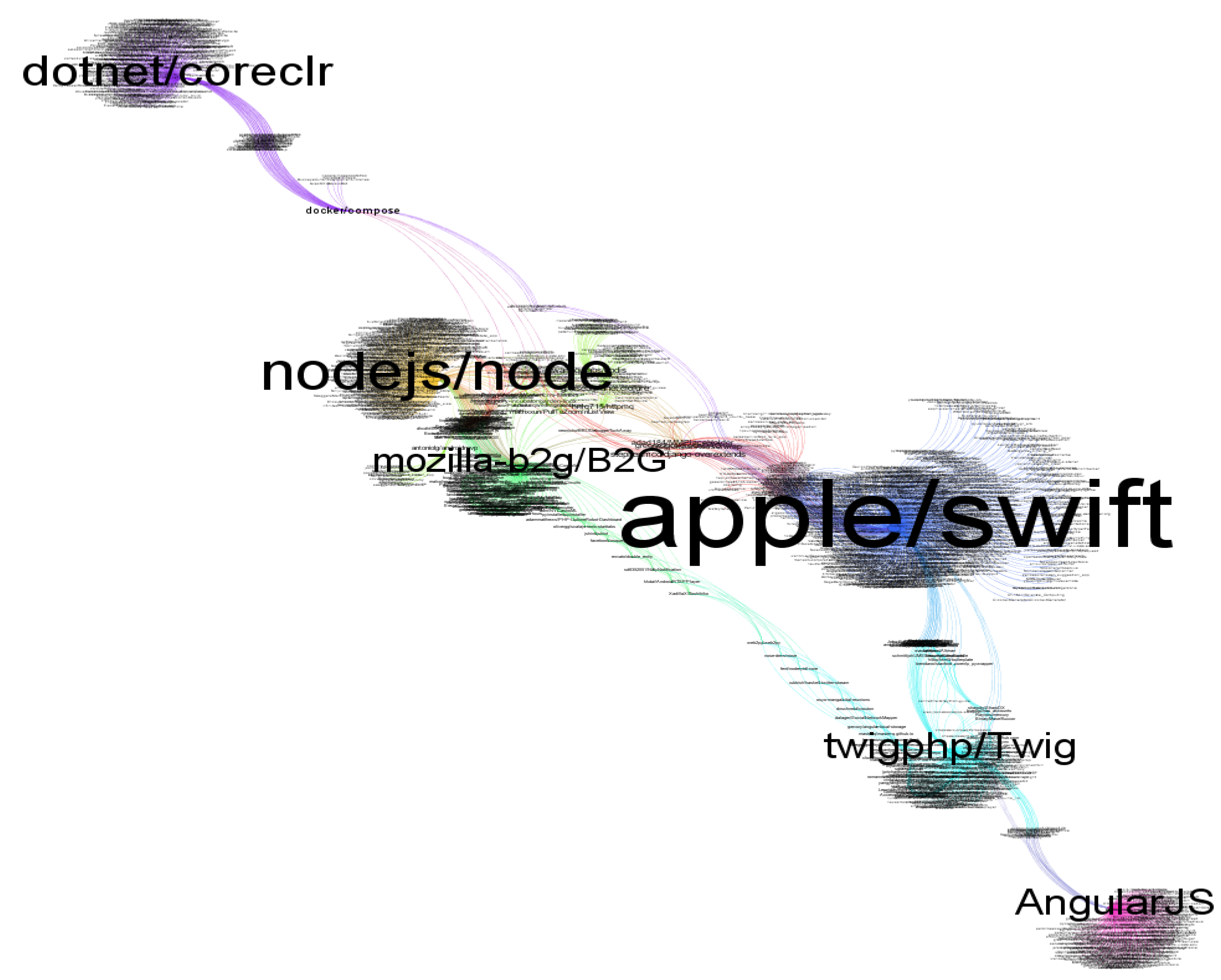
By parsing the project information and interactive information of 10,133 projects that we collected, we obtained a complicated software ecosystem of GitHub projects. To identify the properties of the ecosystem, we analyzed visualizations of the project-relevance network. We used CP–SC to divide the network. Finally, we used Gephi to create a visualization. Figure 4 shows the constructed software ecosystem of GitHub projects.
From Figure 4, we see several projects playing more prominent roles in the ecosystem, such as node, B2G, swift, and Twig. Table 1 shows the details of the top 10 prominent projects with the most dependencies in the GitHub ecosystem. These projects include the fields of open-source tools, programming languages, and development tools. Out of these, development tools account for the largest number.
3.4.2. Distribution of Degree and Conductance
We computed the degree of each project, i.e., the number of nodes that are directly connected to it, and calculated the conductance of each project.
From Figure 5, we find that the degree distribution in the project-relevance network follows the power law. There is a very small number of nodes with a high degree, and a large number of nodes with a low degree. That is to say, only a few projects have a larger number of connections. Combined with Figure 6, we find that the smaller the conductance is, the greater the degree of the node.
3.4.3. Performance of CP–SC
We chose the FastUnfolding, CNM, LPA, Infomap, and SC algorithms to compare with CP–SC that is proposed in this paper. We ran these algorithms five times and obtained the average. The evaluation metrics were modularity, normalized mutual information, and runtime. For the convenience of comparison, we added the Dolphin Social Network data provided by another paper [19], and the NCAA College Football Network data, provided by the paper in Reference [20].
From Table 2, we find that modularity Q of the division results obtained by CNM and FastUnfolding is higher because these two algorithms belong to the modularity-optimization algorithm. Modularity Q generated by the partition of the CP–SC algorithm was higher than that of the SC algorithm, but there was a minor difference with the modular optimization algorithm.
Figure 7 shows the NMI of the CP–SC algorithm and other algorithms, which measures the quality of the division results, on the three datasets of our project network, the football network, and the dolphin network. We found that CP–SC and SC had the best accuracy. Especially in our first dataset GitHub project, CP–SC performed better than the other algorithms.
As shown in Table 3, LPA runs faster than other algorithms. However, from LPA modularity, we can see that LPA is very unstable in terms of community division. The runtime of CP–SC was second only to LPA runtime, but CP–SC had the best accuracy, as can be seen in Figure 7. Thus, CP–SC is better in overall performance.
In general, compared with modularity-optimization algorithms, the CP–SC algorithm does not achieve large modularity Q, but its NMI is better than the other algorithms, and its runtime is second only to the runtime of LPA. Thus, its overall performance is better, and it is more consistent with the development direction of a community-detection algorithm.
4. Influence Of Project Information and Interactive Information
RQ3: Which from project information and interactive information has a larger impact on project relevance?
4.1. Research Method
In order to explore the influence of the two metrics of project information and interaction information on ecosystem identification, we separately constructed the similarity matrix of the two metrics based on their topic-project matrix.
represents the single-dimension project-information similarity matrix. represents the interactive-information similarity matrix. We give different correlation coefficients k, and l to merge similarity matrix, which is denoted by .
Project information and interactive information are the necessary information to construct the similarity matrix. After a lot of experiments, we set 0.8 and 0.2 as the most suitable correlation coefficients in order to make one kind of indicator information have greater impact on the weights between projects. At the same time, other indicator information has little impact on it. Known by the formula , , project information occupies a dominant position that has larger impact on project relevance. On the other side, , , interactive information occupies a dominant position, which has larger impact on project relevance. Finally, we used CP–SC to divide our new relevance network based on the merged similarity matrix and compare with the results of the Section 3.
4.2. Results
Table 4 shows the Pearson correlation between a project-/interactive-information network and project-relevance network. In general, a project-information network has weak association with a project-relevance network, but an interactive-information network has a very strong association with a project-relevance network.
Figure 8 shows the project-information network that is quite different from the project-relevance network. Communities do not have a central project and the network is very sparse. As shown in Figure 9, on the other hand, an interactive-information network is much more densely connected. There is little difference from the project-relevance network. The results indicate that interactive information has a larger impact on project relevance.
5. Discussion
We studied multisource information extraction from GitHub and used our proposed Topic-based Project Knowledge Metrics Framework to construct a topic-project matrix based on topic model LDA; the performance of TPKMF depends on the project history. If there is not enough project information and interactive-information text data, TPKMF has poor performance, especially when meeting a new project.
Our approach collected GitHub’s multisource data, including project information and interactive information, to identify interdependencies between projects. An important step in our TPKMF is to construct a topic-project matrix through topic model LDA. LDA can perform potential text semantic analysis for project text, which provides a bridge for us to analyze project relevance; thus, our TPKMF for analyzing project relevance is logical. Methods that identify interdependencies between projects through code or configuration-file analysis may not be best suited for identifying software ecosystems. For instance, when one project uses the source code of another project, it does not necessarily mean the two software projects evolve together in the same environment. Thus, identifying interdependencies between projects through code or configuration-file analysis may not beimportant for software-ecosystem identification.
In this paper, we introduced the concept of node conductance and proposed the CP–SC algorithm, as well as designed experiments and analyzed the results. CP–SC computes conductance and mines k cluster centers with relatively small conductance, while being relatively decentralized in the network. Finally, we clustered eigenvector of top-k small eigenvalue of Laplace matrix by using K-means, and community division is obtained. The final step of spectral clustering is to obtain community division by K-means. If the number of network communities is large, and the initial clustering center nodes are not well-selected, then the spectral-clustering algorithm often produces poor results. Thus, we improved the spectral-clustering algorithm and proposed a Sone based on the Core Project (CP–SC) to initialize the cluster center nodes by the measuremen methodt based on the core project.
Experiments show that the CP–SC algorithm does not achieve a larger modularity Q than the modularity-optimization algorithm. For instance, Blincoe et al. used the FastUnfolding algorithm in GitHub to divide the project-dependency network and identify 43 ecosystems. Compared with their results, we identified 35 ecosystems with our CP–SC, and about one-third of them are consistent with their results. However, considering NMI and runtime, CP–SC is better than FastUnfolding. Thus, the CP–SC algorithm has the best overall performance.
6. Related Work
6.1. Research on Software Ecosystems
In recent years, software-ecosystem research has been a rapidly developing new phenomenon in the field of software engineering. Early research on software ecosystems mainly concentrates on their definition and limitations [21,22]. In addition to these conceptual explorations related to software ecosystems, many scholars have also analyzed the characteristics of specific software ecosystems. German et al. [23] compared the core code packages and user development packages in the R ecosystem and found that the user development package is smaller, but package size remains stable. Matragkas et al. [24] used clustering algorithms to analyze the ’biodiversity’ features of an open-source-software ecosystem in GitHub, and found that there are three core roles: core developers, active users, and nonactive users. Thomas et al. [25] measured the security of many types of devices in the Android ecosystem and believe that Android’s security relies on system updates. Other research foci include the health measurement of software ecosystems [26], the software architecture of software ecosystems [27], and their organizational business [28]. Libing Deng et al. [29] constructing the Evaluation Indicators System to measure the overall state of the ecosystem. Dayu He et al. [30] analyzed the characteristics of issues in the GitHub open-source ecosystem through visualization technology.
However, these studies rarely involve ecosystem identification, which is the focus of this study.
6.2. Analysis Project Correlation
The main task of identifying software ecosystems is to mine out a subset of projects with similar attributes, i.e., analysis project correlation. In a software ecosystem, Ossher and Businge extracted project-technology dependency relationship from the source code to identify the ecosystem, but this method needs a lot of computation, memory, and time [5,6], which is not suitable for a large-scale project set. Santana and others obtained technical-dependency information by analyzing the configuration files in the project, but this information is not always obtainable [8], which has some limitations. Thung et al. [31] constructed a project-to-project network for GitHub-hosted projects. The edges between projects in the network represent a developer who contributes to both projects. The shared developers do not recognize project dependencies based on this method, so it cannot be used to detect correlation relationships between projects. Kelly Blincoe et al. [11] proposed a reference-coupling way to explore the correlation between the projects in GitHub, which is found in the comments among the projects specified by the user link, but the specified link is little or outdated. Decan et al. [32] studied and analyzed the distribution of R packages and the dependency of cross-library packages in an R language ecosystem in GitHub. Benhong Zhao et al. [33] proposed a prediction model of the project life-span to help developers reschedule the project in open-source-software ecosystems.
6.3. Social Networks in Software Ecosystems
Each ecosystem has a core project. At present, the latest community-detection method can also be applied to the identification of ecosystems. For example, Blincoe et al. use Louvain [34] algorithm in GitHub to divide the project dependency network, 43 ecosystems are identified, including the node ecosystem and the rail ecosystem. Yu et al. [35] used a community-detection algorithm to detect communities in GitHub projects to discover relations between developers. As for other community discovery methods, such as Cai and Li et al. [36] proposed a generalized stochastic block model to find all contact mode in the network, the generalized stochastic block model assumes that the nodes in the network have two forms, one is core node, another is outlier, identifying the generalized community in the network according to different manifestations of nodes. Newman et al. proposed an algorithm for finding the center-edge structure [37] based on the generalized random block model, and proposed a discovering generalized structure algorithms [38]. Chen et al. [39] studied the community-recovery problem in local graphs and proposed two algorithms that are compatible with ring, linear, and small-world graph structures. Barber [40] proposed a combination of the modularity label propagation algorithm (LPAM) to detect large communities by introducing jump attenuation and node preference.
7. Conclusions and Future Work
Software ecosystems have become an area of interest in recent research. Software-ecosystem identification introduces a new paradigm into software-ecosystem research. The projects in an ecosystem are of different importance in playing a vital role on the development of the ecosystem. The primary task of ecosystem identification is to analyze project relevance.
In this paper, we proposed a Topic-based Project Knowledge metrics framework to explore the correlation between projects. Then, we used our improved spectral-clustering algorithm CP-SC to divide the community and obtain a good outcome. Our method verifies that most ecosystems are centered around a core project, and every other ecosystem project is also closely linked to core projects, and the ecosystem is also inter-related. Finally, we can see that the influence of project correlation of the GitHub ecosystem is mainly determined by developer interaction. That is to say, their interaction largely determines the quality and efficiency of ecosystem development; a good interaction between developers makes the ecosystem have more sustainable development.
In future work, we plan to employ other methods to analyze project relevance in software ecosystems, such as deep learning, and explore which projects are most influential and popular. When we encounter new projects, we aim to recommend them to the proper developers, since software ecosystems are not invariable, and their internal structure and operation mode are constantly changing as the time goes by. Thus, our next step is to explore the evolution of these ecosystems after we identify them. In addition, the identification method proposed in this paper opens the door for future research in other open-source platforms.
Author Contributions
All authors discussed the required algorithm to complete the manuscript. Z.L. and S.L. conceived the paper. N.W. performed the experiments and wrote the paper. Q.Z. and Y.Z. checked for typographical errors.
Funding
The works that are described in this paper are supported by NSF 61876190, Ministry of Science and Technology: Key Research and Development Project (2018YFB003800, Hunan Provincial Key Laboratory of Finance and Economics Big Data Science and Technology (Hunan University of Finance and Economics), 2017TP1025 and HNNSF 2018JJ2535.
Acknowledgments
We would like to thank the referees for their valuable comments and suggestions.
Conflicts of Interest
The authors declare no conflict of interest.
References
- Jin, Z.; Zhou, M.; Zhang, Y. Open source software and its eco-systems: Today and tommorow. Sci. Technol. Rev. 2016, 34, 42–48. [Google Scholar]
- Lungu, M.F. Reverse Engineering Software Ecosystems. Ph.D. Thesis, Università della Svizzera italiana, Lugano, Switzerland, 2009. [Google Scholar]
- Cosentino, V.; Izquierdo, J.L.C.; Cabot, J. A Systematic Mapping Study of Software Development with GitHub. IEEE Access 2017, 5, 7173–7192. [Google Scholar] [CrossRef]
- Lungu, M.; Robbes, R.; Lanza, M. Recovering inter-project dependencies in software ecosystems. In Proceedings of the IEEE/ACM International Conference on Automated Software Engineering, Antwerp, Belgium, 20–24 September 2010; pp. 309–312. [Google Scholar]
- Ossher, J.; Bajracharya, S.; Lopes, C. Automated dependency resolution for open source software. In Proceedings of the 2010 7th IEEE Working Conference on Mining Software Repositories (MSR 2010), Cape Town, South Africa, 2–3 May 2010; pp. 130–140. [Google Scholar]
- Brand, M.V.D.; Serebrenik, A.; Businge, J. Survival of Eclipse third-party plug-ins. In Proceedings of the 2012 28th IEEE International Conference on Software Maintenance (ICSM), Trento, Italy, 23–28 September 2012; pp. 368–377. [Google Scholar]
- Mockus, A. Amassing and indexing a large sample of version control systems: Towards the census of public source code history. In Proceedings of the 2009 6th IEEE International Working Conference on Mining Software Repositories (2009), Vancouver, BC, Canada, 16–17 May 2009; pp. 11–20. [Google Scholar]
- Gonzalez-Barahona, J.M.; Robles, G.; Michlmayr, M.; Amor, J.J.; German, D.M. Macrolevel software evolution: A case study of a large software compilation. Empir. Softw. Eng. 2009, 14, 262–285. [Google Scholar] [CrossRef]
- Bavota, G.; Canfora, G.; Penta, M.D.; Oliveto, R.; Panichella, S. How the Apache community upgrades dependencies: An evolutionary study. Empir. Softw. Eng. 2015, 20, 1275–1317. [Google Scholar] [CrossRef]
- German, D.M.; Gonzlezbarahona, J.M.; Robles, G. A Model to Understand the Building and Running Inter-Dependencies of Software. In Proceedings of the 14th Working Conference on Reverse Engineering (WCRE 2007), Vancouver, BC, Canada, 28–31 Octorber 2007; pp. 140–149. [Google Scholar]
- Blincoe, K.; Harrison, F.; Damian, D. Ecosystems in GitHub and a Method for Ecosystem Identification Using Reference Coupling. In Proceedings of the 2015 IEEE/ACM 12th Working Conference on Mining Software Repositories, Florence, Italy, 16–17 May 2015. [Google Scholar]
- Blei, D.M.; Ng, A.Y.; Jordan, M.I. Latent dirichlet allocation. J. Mach. Learn. Res. Arch. 2003, 3, 993–1022. [Google Scholar]
- Rachman, Z.A.; Maharani, W. The analysis and implementation of degree centrality in weighted graph in Social Network Analysis. In Proceedings of the 2013 International Conference of Information and Communication Technology (ICoICT), Bandung, Indonesia, 20–22 March 2013. [Google Scholar]
- Taylor, I.W.; Rune, L.; David, W.F.; Yongmei, L.; Catia, P.; Daniel, F.; Shelley, B.; Tony, P.; Quaid, M.; Wrana, J.L. Dynamic modularity in protein interaction networks predicts breast cancer outcome. Nat. BioTechnol. 2009, 27, 199–204. [Google Scholar] [CrossRef] [PubMed]
- Mcdaid, A.F.; Greene, D.; Hurley, N. Normalized Mutual Information to evaluate overlapping community finding algorithms. arXiv, 2011; arXiv:1110.2515. [Google Scholar]
- Adler, J.; Parmryd, I. Quantifying colocalization by correlation: The Pearson correlation coefficient is superior to the Mander’s overlap coefficient. Cytometry Part A 2010, 77, 733–742. [Google Scholar] [CrossRef] [PubMed]
- Newman, M.E.J. Modularity and community structure in networks. Proc. Natl. Acad. Sci. USA 2006, 103, 8577–8582. [Google Scholar] [CrossRef] [PubMed] [Green Version]
- Kuncheva, L.I.; Hadjitodorov, S.T. Using diversity in cluster ensembles. In Proceedings of the 2004 IEEE International Conference on Systems, Man and Cybernetics, Hague, The Netherlands, 10–13 Octorber 2004; pp. 1214–1219. [Google Scholar]
- Lusseau, D. The emergent properties of a dolphin social network. Proc. Biol. Sci. 2003, 270 (Suppl. 2), S186. [Google Scholar] [CrossRef] [PubMed]
- Girvan, M.; Newman, M.E.J. Community structure in social and biological networks. Proc. Natl. Acad. Sci. USA 2002, 99, 7821–7826. [Google Scholar] [CrossRef] [PubMed] [Green Version]
- Jansen, S.; Finkelstein, A.; Brinkkemper, S. A sense of community: A research agenda for software ecosystems. In Proceedings of the 2009 31st International Conference on Software Engineering, Vancouver, BC, Canada, 16–24 May 2009; pp. 187–190. [Google Scholar]
- Bosch, J.; Bosch-Sijtsema, P.M. Softwares Product Lines, Global Development and Ecosystems: Collaboration in Software Engineering; Springer: Berlin/Heidelberg, Germany, 2010; pp. 360–368. [Google Scholar]
- German, D.M.; Adams, B.; Hassan, A.E. The Evolution of the R Software Ecosystem. In Proceedings of the 2013 17th European Conference on Software Maintenance and Reengineering, Genova, Italy, 5–8 March 2013; pp. 243–252. [Google Scholar]
- Matragkas, N.; Williams, J.R.; Kolovos, D.S.; Paige, R.F. Analysing the ’biodiversity’ of open source ecosystems: The GitHub case. In Proceedings of the 11th Working Conference on Mining Software Repositories, Hyderabad, India, 31 May–1 June 2014; pp. 356–359. [Google Scholar]
- Thomas, D.R.; Beresford, A.R.; Rice, A. Security Metrics for the Android Ecosystem. In Proceedings of the 5th Annual ACM CCS Workshop on Security and Privacy in Smartphones and Mobile Devices, Denver, CO, USA, 12–15 October 2015; pp. 87–98. [Google Scholar]
- Manikas, K.; Hansen, K.M. Reviewing the Health of Software Ecosystems—A Conceptual Framework Proposal. In Proceedings of the 5th International Workshop on Software Ecosystems, Potsdam, Germany, 11–14 June 2013. [Google Scholar]
- Viljainen, M.; Kauppinen, M. Software Ecosystems: A Set of Management Practices for Platform Integrators in the Telecom Industry; Springer: Berlin/Heidelberg, Germany, 2011; pp. 32–43. [Google Scholar]
- Scacchi, W.; Alspaugh, T.A. Understanding the role of licenses and evolution in open architecture software ecosystems. J. Syst. Softw. 2012, 85, 1479–1494. [Google Scholar] [CrossRef]
- Liao, Z.; Deng, L.; Fan, X.; Zhang, Y.; Liu, H.; Qi, X.; Zhou, Y. Empirical Research on the Evaluation Model and Method of Sustainability of the Open Source Ecosystem. Symmetry 2018, 10, 747. [Google Scholar] [CrossRef]
- Liao, Z.; He, D.; Chen, Z.; Fan, X.; Zhang, Y.; Liu, S. Exploring the Characteristics of Issue-related Behaviors in GitHub Using Visualization Techniques. IEEE Access 2018, 6, 24003–24015. [Google Scholar] [CrossRef]
- Thung, F.; Bissyande, T.F.; Lo, D.; Jiang, L. Network Structure of Social Coding in GitHub. In Proceedings of the 2013 17th European Conference on Software Maintenance and Reengineering, Genova, Italy, 5–8 March 2013; pp. 323–326. [Google Scholar]
- Decan, A.; Mens, T.; Claes, M.; Grosjean, P. When GitHub Meets CRAN: An Analysis of Inter-Repository Package Dependency Problems. In Proceedings of the 2016 IEEE 23rd International Conference on Software Analysis, Evolution, and Reengineering, Osaka, Japan, 14–18 March 2016; pp. 493–504. [Google Scholar]
- Liao, Z.; Zhao, B.; Liu, S.; Jin, H.; He, D.; Yang, L.; Zhang, Y.; Wu, J. A Prediction Model of the Project Life-Span in Open Source Software Ecosystem. Mob. Netw. Appl. 2017. [Google Scholar] [CrossRef]
- Blondel, V.D.; Guillaume, J.L.; Lambiotte, R.; Lefebvre, E. Fast unfolding of communities in large networks. J. Stat. Mech. 2008, 2008, 155–168. [Google Scholar] [CrossRef]
- Yu, Y.; Yin, G.; Wang, H.; Wang, T. Exploring the patterns of social behavior in GitHub. In Proceedings of the 1st International Workshop on Crowd-based Software Development Methods and Technologies, Hong Kong, China, 17–19 November 2014; pp. 31–36. [Google Scholar]
- Cai, T.T.; Li, X. Robust and computationally feasible community detection in the presence of arbitrary outlier nodes. Ann. Stat. 2015, 43, 5–24. [Google Scholar] [CrossRef]
- Xiao, Z.; Travis, M.; Newman, M.E.J. Identification of core-periphery structure in networks. Phys. Rev. E Stat. Nonlinear Soft Matter Phys. 2014, 91, 784321–784331. [Google Scholar]
- Newman, M.E.; Peixoto, T.P. Generalized Communities in Networks. Phys. Rev. Lett. 2015, 115, 088701. [Google Scholar] [CrossRef] [PubMed] [Green Version]
- Chen, Y.; Kamath, G.; Suh, C.; Tse, D. Community Recovery in Graphs with Locality. In Proceedings of the 33rd International Conference on Machine Learning, New York, NY, USA, 19–24 June 2016. [Google Scholar]
- Barber, M.J.; Clark, J.W. Detecting network communities by propagating labels under constraints. Phys. Rev. E Stat. Nonlinear Soft Matter Phys. 2009, 80, 026129. [Google Scholar] [CrossRef] [PubMed]
Figure 1.
Topic-based Project Knowledge Metrics Framework (TPKMF) buildsthe topic–project relation matrix by LDA.
Figure 1.
Topic-based Project Knowledge Metrics Framework (TPKMF) buildsthe topic–project relation matrix by LDA.

Figure 2.
Project-relevance networks with different degrees.

Figure 3.
Visualization of the proposed Core Project–Spectral Clustering (CP–SC) algorithm. CP–SC can mainly be summarized as two steps: First, according to the size of the conductance, nodes are sorted from large to small (the smaller the conductance, the larger the node). Then, selecting k nodes with minimum conductance and k-dimensional Euclidean distance between them that is larger than given distance threshold (nodes marked in red are selected k initial cluster centers). Finally, running the k-means algorithm on spectral-clustering division vector .

Figure 4.
Ecosystems in GitHub. Different colors represent different divided ecosystems. Project names follow the pattern user/repository, where user is the owner’s GitHub login, and repository is the name of the project repository.
Figure 4.
Ecosystems in GitHub. Different colors represent different divided ecosystems. Project names follow the pattern user/repository, where user is the owner’s GitHub login, and repository is the name of the project repository.

Figure 5.
Degree distribution in the project-relevance network.

Figure 6.
Degree distribution in the project-relevance network.

Figure 7.
Normalized Mutual Information (NMI) comparison between algorithms.

Figure 8.
Project-information network.

Figure 9.
Interactive-information network.


Table 1.
Core projects in the ecosystem.
| Project | Description | Language | Fork | Commits | Ecosystem Size | Total Weight |
|---|---|---|---|---|---|---|
| apple/swift | Open-Source Tool | Swift | 2776 | 6839 | 23.25% | 221 |
| nodejs/node | Development Tool | Java Script | 3418 | 2517 | 17.05% | 198 |
| mozilla-b2g/B2G | Open Source Tool | Python | 176 | 139 | 10.25% | 61 |
| twigphp/Twig | Programming Language | Php | 77 | 83 | 6.28% | 43 |
| angular/angular.js | Programming Language | Java Script | 46 | 59 | 5.48% | 31 |
| dotnet/coreclr | Development Tool | Java | 76 | 49 | 3.69% | 28 |
| collectd/collectd | Framework | Java | 98 | 43 | 1.80% | 18 |
| docker/compose | Development Tool | Python | 126 | 188 | 2.88% | 41 |
| dotnet/compose | Development Tool | Java | 46 | 89 | 0.75% | 11 |
| sharpdx/SharpDX | Framework | Java | 26 | 88 | 0.88% | 21 |
Table 2.
Modularity of community-division results.
| Algorithm | Projects | Dolphins | Football |
|---|---|---|---|
| LPA | 0.375 | 0.478 | 0.611 |
| CNM | 0.411 | 0.525 | 0.580 |
| FastUnfolding | 0.450 | 0.550 | 0.635 |
| Infomap | 0.432 | 0.558 | 0.630 |
| SC | 0.428 () | 0.528 () | 0.605 () |
| CP-SC | 0.430 ( = 0.09) | 0.533 ( = 0.07) | 0.618 ( = 0.05) |
Table 3.
Runtime comparison between algorithms.
| Algorithm (in Seconds) | Projects | Dolphins | Football |
|---|---|---|---|
| LPA | 0.343 | 0.256 | 0.782 |
| CNM | 0.672 | 0.532 | 1.470 |
| FastUnfolding | 1.242 | 1.180 | 2.248 |
| Infomap | 1.472 | 1.238 | 2.835 |
| SC | 1.788 (k = 10) | 1.436 (k = 2) | 2.495 (k = 12) |
| CP-SC | 0.398 ( = 0.09) | 0.303 ( = 0.07) | 0.647 ( = 0.05) |
Table 4.
Pearson correlation coefficient between two networks.
| Project Relevance Network | Coefficient | |
|---|---|---|
| Project Information Network | 0.228 | , |
| Interactive Information Network | 0.813 | , |
© 2019 by the authors. Licensee MDPI, Basel, Switzerland. This article is an open access article distributed under the terms and conditions of the Creative Commons Attribution (CC BY) license (http://creativecommons.org/licenses/by/4.0/).
Share and Cite
MDPI and ACS Style
Liao, Z.; Wang, N.; Liu, S.; Zhang, Y.; Liu, H.; Zhang, Q. Identification-Method Research for Open-Source Software Ecosystems. Symmetry 2019, 11, 182. https://doi.org/10.3390/sym11020182
AMA Style
Liao Z, Wang N, Liu S, Zhang Y, Liu H, Zhang Q. Identification-Method Research for Open-Source Software Ecosystems. Symmetry. 2019; 11(2):182. https://doi.org/10.3390/sym11020182
Chicago/Turabian StyleLiao, Zhifang, Ningwei Wang, Shengzong Liu, Yan Zhang, Hui Liu, and Qi Zhang. 2019. "Identification-Method Research for Open-Source Software Ecosystems" Symmetry 11, no. 2: 182. https://doi.org/10.3390/sym11020182
Note that from the first issue of 2016, this journal uses article numbers instead of page numbers. See further details here.