Estimation at Completion Simulation Using the Potential of Soft Computing Models: Case Study of Construction Engineering Projects

Abstract

“Estimation at completion” (EAC) is a manager’s projection of a project’s total cost at its completion. It is an important tool for monitoring a project’s performance and risk. Executives usually make high-level decisions on a project, but they may have gaps in the technical knowledge which may cause errors in their decisions. In this current study, the authors implemented new coupled intelligence models, namely global harmony search (GHS) and brute force (BF) integrated with extreme learning machine (ELM) for modeling the project construction estimation at completion. GHS and BF were used to abstract the substantial influential attributes toward the EAC dependent variable, whereas the effectiveness of ELM as a novel predictive model for the investigated application was demonstrated. As a benchmark model, a classical artificial neural network (ANN) was developed to validate the new ELM model in terms of the prediction accuracy. The predictive models were applied using historical information related to construction projects gathered from the United Arab Emirates (UAE). The study investigated the application of the proposed coupled model in determining the EAC and calculated the tendency of a change in the forecast model monitor. The main goal of the investigated model was to produce a reliable trend of EAC estimates which can aid project managers in improving the effectiveness of project costs control. The results demonstrated a noticeable implementation of the GHS-ELM and BF-ELM over the classical and hybridized ANN models.

1. Introduction

Poor performances have often been recorded in project management due to its risky nature. The constant environmental changes and other external constraints have made risk management a serious issue in the construction industry [1,2]. Project monitoring must be given adequate attention, (in terms of the close monitoring and detection of deviations and of taking appropriate measures to address any deviations) in order to make profit. Meanwhile, the initial stage of most construction activities focusses on budget planning, effectively neglecting the impact of changes in the engineering cost and the updating of information during construction [3], and this has prevented an effective detection of the problems associated with project cost control. Owing to the dynamic nature of project conditions upon the commencement of a project, there is a need for a regular revision of the project budget for an effective project execution.

One of the managerial and monitoring tools used by project managers is the Earned Value Management (EVM) [4,5]. The EVM can facilitate the management of the 3 critical elements of project management (scope, time, and cost) [6]. Most project managers depend on EVM to estimate the project completion time (EAC) and to make a quick evaluation of the costs of completing scheduled project activities [7]. The estimated EAC can help managers to determine the differences between the actual and planned projects costs to resolve any underlying problems. A brief description of the EAC process during the life of a project is displayed in Figure 1.

The practical computation of the EAC demands that managers must first collect data relating to project cost management before using formulas to execute the calculations [8]. The major disadvantage of using formulas for EAC calculation is the numerous available methods for EAC calculations. There are about eight EAC calculation methods in the literature [9]; hence, it is the duty of the managers to judiciously decide the best calculation method that will suit their demands. Project costs are influenced by several factors, and each project has its own unique characteristics. Therefore, there is a need to select the best formula that will suit each case. Various regression-based approaches have been developed as an alternative to the index-based approach as advantageous methodologies for performing cost estimation activities [10,11,12]. The determination of the estimation at completion using soft computing models where the regression problem is introduced and solved and the dependent attribute variables (typically the actual project cost) against an independent variable (a predictor, typically time) configured using nonlinear modeling solution where the respective relationship between the predictor and the response are established.

Due to the uncertain and context-dependent nature of construction projects, it is usually expensive to develop deterministic models for EAC prediction. In this case, an approximate inference which is cost effective and fast may be the viable alternative [13]. Inference models are used to formulate new facts from historical data, and its processes adaptively changes when the historical data are altered. The human brain is naturally endowed with the capacity of inferring new facts from information previously acquired. Therefore, models which can simulate the inference ability of the human brain can be developed using artificial intelligence (AI). The concept of the AI implies that computer systems can handle complex or ill-structured problems using specialized techniques like Artificial Neural Network (ANN), fuzzy logic, or Support Vector Machine (SVM). Since AI-aided computer systems can operate as humans, it may be viable to deploy AI inference models as a tool for handling EAC problems. While trying to construct AI models to handle EAC problems, EAC forecasting has itself been found to be characterized by several uncertainties, and one of these uncertainties is the huge variable data that characterize construction costs. Besides, there are other factors that influence project cost, such as site productivity, weather, and socioeconomic constraints. The individual prediction of these factors is either tedious or near impractical. Therefore, forecasting models must be able to cope with these influencing factors to achieve a desirable EAC prediction.

Cost overrun is a common problem frequently encountered during the construction phase of a project. Hence, there is a need for a proactive monitoring of project costs to identify foreseeable problems. EAC assists project managers in the identification of potential problems and helps them to plan for the appropriate measures to address them.

The earned value management (EVM) is the predominant method applied by the project managers for the construction industry to trail the project status and to measure the performance of the project [14]. The actual mechanism of this method is to configure the actual relationship between the planned resource and the targeted project goals. Even though the EVM method is widely implemented for project control, EVM is associated with several limitations. Numerous studies have been established to enhance the main concept of EVM.

An examination of the likeliness of organizing the data envelope analysis (DEA) approach is conducted for the evaluation of the project performances in a multi-project situation [15]. The investigated modeling approach is performed based on EVM and the multidimensional control system. An attempt on the refinement and improvement of the performance of the conventional EVM through the introduction of statistical control chart techniques has been made by Reference [16]. The authors established a control chart for the monitoring of the project performance through a timely detection system. Another study was performed to improve the ability of project managers to give an informative project decisions [17]. Plaza and Turetken (2009) suggested the influence of learning on the performance of a project team through an enhanced version of EVM [18]. Pajares and López-Paredes (2011) integrated risk management techniques with the EVM method to develop two new strategies to identify the project overruns [19]. Despite all these attempts to improve the EVM, there are still drawbacks that require more efforts in order to come up with a better solution. Based on the latest review research on the project cost and earned value management conducted by [20], the authors identified 455 articles on this subject and examined 187 papers in their study. The scholars classified the methodologies applied on the project cost monitoring into (i) observational analysis, (ii) extended EVM analysis, (iii) statistical analysis, (iv) artificial intelligence (AI), and (v) computerized analysis. AI models were recognized as the prevailing reliable implemented control system, yet investigations on the application of these models on project performance control are still in the early stages.

For a better visualization and analysis for the state-of-the-art AI models on cost project management,

Table 1. The surveyed literature of artificial intelligence models’ implementation on cost projects over the last decade.

References	Research Remark
[25]	The study was conducted on the usage of the Artificial Neural Network (ANN) model to simulate project cost with the aim to improve the earned value management (EVM) system. The finding evidenced the applicability of the intelligent model to minimize the project cost overruns.
[26]	An integration of support vector machine with fast messy genetic algorithm (SVM-FMGA) was performed for construction management monitoring. The validation of the model approved the estimation of the building cost over the conceptual cost estimation.
[27]	The study inspected a conceptual cost estimation using the evolutionary fuzzy hybrid neural network for industrial project construction. The research outcomes exhibited another optimistic finding for a precise cost estimation at the early stages.
[28]	An independent intelligent based on the weighted support vector machine model and fuzzy logic set was studied for EAC prediction. The fuzzy model was applied to solve the associated uncertainty in the tie series data.
[29]	A fuzzy neural network was used to determine the EAC. The modeling was piloted based on various factors (both qualitative and quantitative) that influence the EAC value. The results demonstrated good outcomes from the contractors and managers aspects.
[30]	The authors investigated a relatively new model based on the Bayesian theory integrated with the EVM framework aiming to compute the EAC. The proposed model evidenced its applicability and effectiveness on modeling the estimation at completion.
[10]	The scholars developed a new cost EAC methodology by integrating the Cost Estimate at Completion (CEAC) method and four growth models and concluded that the EAC formula based on the Gompertz model outperforms the other indexed formulas.
[31]	The support vector regression model was analyzed to perform the EVM. The authors concluded that their model outperformed the available best performing EVM methods through the training of the identical data set.
[32]	An automotive programming approach based on the ANN model was proposed for estimating the EAC element of a dam construction project. The results demonstrated a remarkable performance for the investigated case study.

tabulates all the conducted studies over the past decade, with a research remark for each. AI models are presented as a reliable alternative modeling strategy to overcome the problems associated with the indexed procedures to compute the EAC. AI models are distinguished by their capability of solving complex problems by imitating the analytical capability of the human brain. Over the past thirty years, there has been a massive successful utilization of AI models in several areas of science and engineering.

Although there have been several investigations since 2008 on cost project estimation using AI models, the topic is still associated with various limitations and requires more efforts from scholars to figure out new solutions with more robust/concrete modeling strategies. Based on the presented researches in Table 1, a few studies have been explored for EAC prediction. Also, these studies reported several limitations of the AI model, such as the black-box nature, the requirement of a significant amount of data, overfitting, models’ interaction, and time consumption [21]. Among several AI models, the artificial neural network, support vector machine, and adaptive neuro-fuzzy inference system have been majorly used.

A new version of ANN called extreme learning machine (ELM) model was proposed by Reference [22]. Over the past three years, the ELM model has been improved and applied to multiple engineering applications and with more applicability for solving complex problems characterized by non-linear and stochasticity behaviors [23,24]. The massive and solid implementation of the ELM model encouraged the main authors of this current research to develop this model for EAC simulation with the aim of achieving a robust expert system for construction project management sustainability.

Based on the identified limitations of the existing AI models, it is highly encouraging to explore more reliable, robust, and trustful methodologies to solve the project cost overruns during project execution. Historical data were collected from several construction projects and used to inspect the predictability of the proposed model. The projects’ information was used to set up the trend of a project cost flow and the relationship between the project EAC and monthly costs we mapped based on historical knowledge and experience. The research objectives are summarized in threefold:

• A new intelligence model called extreme learning machine was introduced to the model EAC.
• The predictability of the ELM model in computing EAC was validated against the traditional artificial neural network.
• The predictive ELM model was improved by input attribute optimization approaches called global harmony search and brute force for the identification of the factors that significantly affect project cost.
• Overall, the research explored a new modeling strategy based on the coupled intelligence model which can assist project managers in making decisions.

2. Materials and Methods

2.1. Extreme Learning Machine (ELM) Model

Owing to the issues of the conventional machine learning models (e.g., ANN), the ELM was proposed as a new technique to address these problems [24,26]. In this context, the term “extreme” depicts a high capability of the algorithm to mimic the behavior of the human brain within a short modeling time [33]. The ELM has a simple and unique learning process because the hidden neurons do not require any tuning process during the learning phase [22]. Contrarily, human intervention is required in the conventional learning methods like the ANN or SVM, especially in establishing the most appropriate model parameters. The ELM has an advantage over the conventional data-intelligent models framework due to its role in formulating data-intelligent expert systems for application in real-life situations (e.g., in References [27,28]). The ELM has, over the last five years, been used in solving several problems, such as clustering [34], feature learning, classification, and regression [35] with a significant level of performance and learning capacity [36,37,38,39,40,41,42,43,44].

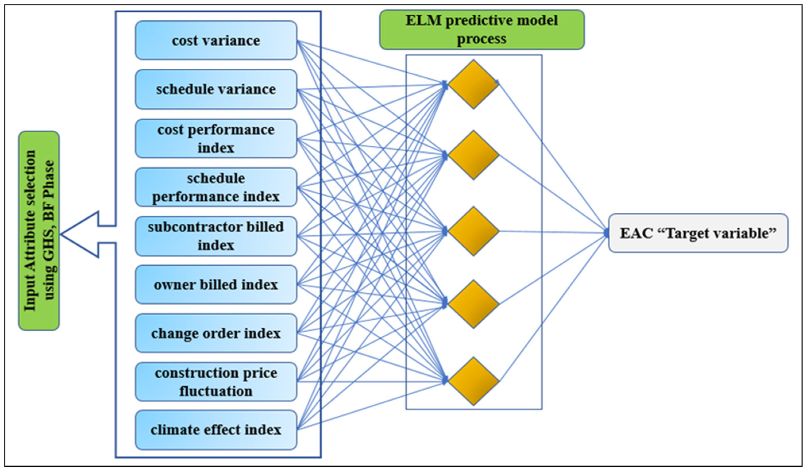
Up to date, studies on the predictive ability of the ELM in modeling project management applications are yet to be reported. Hence, in this work, the novelty of the ELM lies in its rapid rate of learning based on the single layer feedforward network (SLFN). It can also generalize data features with greater efficiency compared to other soft computing techniques [43]. Figure 2 displayed the graphical representation of the ELM general architecture for the applied application.

Based on this figure, the input parameters in this study are cost variance (CV), schedule variance (SV), cost performance index (CPI), schedule performance index (SPI), subcontractor billed index, owner billed index, change order index, construction price fluctuation (CCI), and climate effect index while the EAC is the response that will be evaluated. The input and output variables are connected by the hidden nodes in the phase space in a fashion that allows features determination by the randomly generated input and output weights. The trained model was used to model the input-target data set in this study. The modelling phase accounted for 80%, and the testing phase accounted for 20%. The ELM was used to process the input data through an $M$-dimensional mapping feature space which randomly determines the internal weights. The following mathematic procedures governed the output network [22]:

$$F_{\left(x\right)}={{\displaystyle \sum }}_{i=1}^M{\beta }_i{h}_i\left(x\right)$$

(1)

where ${\beta }_i$ represents the weight of the output matrix that connected the targeted phase to the hidden layer space, $h_i$ is the output of the hidden nodes for the input variables $\left(x\right)$, and $M$ is the dimension of the feature space of the ELM [45]. Thus, the ELM model can be used to solve the regression problem that featured the EAC and the various construction project variables. The learning process of the ELM model can be presented in the following form [22]:

$$H\beta =T$$

(2)

where $H$ is the feature space for the “hidden zone output matrix” $M,$ and $T$ defines the target matrix. The ELM learning operation mainly targets at obtaining the least error as per the terms $Minimize:\left|\right|H\beta -T\left|\right|$ and $\left|\right|\beta \left|\right|$ while the hidden output layer $H$ can be expressed as [46]

$$H=\left[\begin{array}{ccc}{h}_1{x}_1& \cdots & h_M{x}_1\\ ⋮& \ddots & ⋮\\ h_1{x}_N& \cdots & h_M{x}_N\end{array}\right]$$

(3)

2.2. Artificial Neural Network (ANN) Model

The ANN is developed as a statistical optimization method that mimics the behavior of the biological nervous system [47,48]. They can generate logical models composed of several neurons that are interconnected in a computing environment. ANNs are ideal in establishing the solutions to complicated modeling problems like classifying, pattern recognition, or estimating [49]. These three modeling procedures are predominately used in the development of any ANN. There are two main forms of ANN for classification or regression tasks; these are supervised and unsupervised ANNs. In the supervised ANNs, training is performed via a regulation of the values of the interneuronal weights so that it will be possible to predict the values of the output after incorporating several input data from the previously executed experiments. For the unsupervised ANNs, no set target values exist while introducing the input into the system. The multilayer perceptron (MLP) feedforward ANN is a common framework for training optimization algorithms and has one or more hidden layers, and the input parameters are selected based on the analysts’ experience and on the type of problem at hand [50]. For the feedforward backpropagation frameworks, the input traverses the network and later match with the output at the end to estimate the level of error [51,52]. In the backpropagation framework, the learning rule ensures that an input–output relationship exists. This relation is usually based on a random allocation of the initial weights to the input data prior to updating. Next, the outcome of the iteration process is compared to the desired output to update the weighted input data.

In most studies, neural computations are employed based on several transfer functions and the type of problem at hand. Recent engineering processes utilize the tangent sigmoid and the linear functions as transfer functions, respectively, for the hidden and output layers. The basis for the application of the tangent sigmoid transfer function to the hidden neurons is to ensure a significant improvement in the systems’ input–output behavior when varying the updated weights.

2.3. Global Harmony Search (GHS) Optimization Algorithm

The global harmony search framework was developed based on the pattern of a musical process when searching for the optimized solution. This algorithm was proposed by Reference [53] for optimizing problems with continuous and discrete variables. In the GHS algorithm, the best harmony is considered as a new harmony memory. One of the applications of the GHS is in searching for the influence of highly dimensional input parameters [54]. In this research and to the best knowledge of the authors, the GHR algorithm is applied as the input variables selection approach for the ELM and ANN predictive model.

2.4. Brute Force Input Optimization Method

Brute force (BF) is a systematic selecting approach for solving problems which requires the enumeration of all the possible features [55] with the aim of achieving a solution to specific problems and checking the suitability of each option towards satisfying the problem statement [56]. BF is usually performed to find the divisors of a number n that would list all the integers from 1 to n and check that each integer will perfectly divide n without any remainder. Although a BF search is easy to implement and will always establish a solution to the problem, its cost is directly related to the number of options considered, and this number tends to grow with the size of the problem in many practical situations. BF is, therefore, applicable in situations where the size of the problem is limited or in the absence of a specific heuristic method that can be used effectively to reduce the number of solutions to a considerable size. The BF approach can also be used as a yardstick for benchmarking the performance of other algorithms. It is considered as one of the simplest search approaches. The selection of this search approach for integration with the developed predictive model was inspired from its potential in feature selection problems.

2.5. Modeling Procedure Phase

The models were applied using historical information related to civil engineering construction projects located in the United Arabian Emirate. The type of the constructions is residential project, and the projects period was between eleven to twelve months. The associated project information was presented in the following forms: schedule variance (SV), cost variance (CV), schedule performance index (SPI), cost performance index (CPI), subcontractor billed index, construction price fluctuation, owner billed index, change order index, and climate effect index. On the other hand, the estimation at completion was organized to be the predict and variable in the learning process. The model was constructed using eleven construction projects with 132 periods; 75 percentage of the total data was for the learning processes of the predictive model whereas 25% (32 period) was used to initiate the testing phase for the modeling evaluation. A full detail of the studied projects is displayed in

Table 2. The details of the modeled construction project used in the current research.

Project Name	Total Area (m2)	Underground Floors	Ground Floors	Buildings	Start Date	Finish Date	Duration (Days)	Contract Amount ($)	Prediction Periods
A	11,254	1	1	3	2 March 2008	24 April 2009	418	7,445,825	13
B	9326	1	1	1	15 August 2008	28 July 2009	347	6,329,548	14
C	12,548	1	1	2	23 April 2003	28 February 2004	311	9,518,465	12
D	9482	0	1	1	10 October 2009	3 November 2010	389	7,458,124	11
E	10,554	2	1	2	5 June 2005	2 July 2006	392	8,452,847	12
F	8751	1	1	2	5 July 2011	30 April 2012	300	6,895,348	14
G	9458	0	1	1	13 August 2005	25 July 2006	346	7,518,452	13
H	13,758	1	1	3	20 September 2004	15 October 2005	390	9,548,249	16
I	11,249	1	1	3	20 April 2007	18 April 2008	364	8,628,945	13
J	7851	0	1	1	24 December 2011	19 January 2013	392	5,936,461	14
Total									132
Training									99
Testing									33

.

The predictive models were examined using several numerical indicators that present the absolute error evaluation (the closest to zero) and the best-goodness (the closest to one). In that way, more justification can be done on the optimal model for the best input combination. The numerical indicators were the root mean square error (RMSE) [57], mean absolute error (MAE), mean relative error (MRE), Nash–Sutcliffe coefficient (NSE) [58], scatter index (SI) [59], and correlation coefficient (R). The mathematical model can be described as follows:

$$RMSE=\sqrt{\frac{{{\displaystyle \sum }}_{i=1}^n{\left(EA{C}_a-EA{C}_p\right)}^2}{n}}$$

(4)

$$MAE=\frac{{{\displaystyle \sum }}_{i=1}^n\left|EA{C}_a-EA{C}_p\right|}{n}$$

(5)

$$MRE=\frac{1}{n}{\displaystyle \sum }_{i=1}^n\left(\frac{EA{C}_a-EA{C}_p}{EA{C}_a}\right)$$

(6)

$$NSE=1-\left[\frac{{{\displaystyle \sum }}_{i=1}^n{\left(EA{C}_a-EA{C}_p\right)}^2}{{{\displaystyle \sum }}_{i=1}^n{\left(EA{C}_a-\overline{EA{C}_a}\right)}^2}\right]$$

(7)

$$SI=\frac{\sqrt{\frac{{{\displaystyle \sum }}_{i=1}^n{\left(EA{C}_a-EA{C}_p\right)}^2}{n}}}{\overline{EA{C}_a}}$$

(8)

$$R=1-\left[\frac{{{\displaystyle \sum }}_{i=1}^n(EA{C}_a-\overline{EA{C}_a})\left(EA{C}_p-\overline{EA{C}_p}\right)}{\sqrt{{{\displaystyle \sum }}_{i=1}^n{(EA{C}_a-\overline{EA{C}_a})}^2}\sqrt{{{\displaystyle \sum }}_{i=1}^n{(EA{C}_p-\overline{EA{C}_p})}^2}}\right]$$

(9)

where $EA{C}_a$ is the actual observation, $EA{C}_p$ is the predicted value, and $\overline{EA{C}_a}$ and $\overline{EA{C}_p}$ are the mean values of the actual and predicted values.

3. Results and Discussions

This section presents the applicability of the hybrid predictive models (i.e., ELM, ANN, GHS-ELM, GHS-ANN, BF-ELM, and BF-ANN) for simulating the estimation at completion of construction projects. As a concluding stage of the prediction process, the data cost of the selected projects was determined by computing the differences between the planned and actual costs for each month. The applied intelligence models were used to compute the mathematical relationship between nine attributes (the abstracted input combinations) and the targeted variable (EAC). The applied hybrid models were used in this computation process to overcome the challenges of the classical indexed formulations. Worth to mention, the hybrid intelligence models have been proven to simulate the human intelligence in finding solutions to complex real-life problems.

Several statistical indicators are used to present the absolute error measures and the best fit goodness as tabulated in

Table 3. The numerical evaluation indicators for the ELM and ANN predictive models “Based-models versions” over the testing modeling phase.

Predictive Models	RMSE	MAE	MRE	NSE	SI	BIAS	R
ELM	0.1492	0.0766	−0.1219	0.5782	0.8750	0.0413	0.8167
ANN	0.2085	0.1036	0.4548	0.1764	1.2227	0.0359	0.5031

,

Table 4. The input combination attributes used to determine the value of the EAC using the GHS-ELM model.

The Number of Inputs	Models	The Type of Input Variables	Output
2 inputs	Model 1	Cost variance (CV), schedule performance index (SPI)	EAC
3 inputs	Model 2	CV, schedule variance (SV), SPI	EAC
4 inputs	Model 3	CV, SV, SPI, Change order index	EAC
5 inputs	Model 4	CV, SV, cost performance index (CPI), SPI, owner billed index	EAC
6 inputs	Model 5	CV, SV, CPI, SPI, owner billed index, change order index	EAC
7 inputs	Model 6	CV, SV, CPI, SPI, subcontractor billed index, change order index, climate effect index	EAC
8 inputs	Model 7	CV, SV, CPI, SPI, subcontractor billed index, owner billed index, change order index, climate effect index	EAC

,

Table 5. The numerical evaluation indicators for the GHS-ELM predictive model over the testing modeling phase (Bold is the best input combination).

Method	RMSE	MAE	MRE	NSE	SI	BIAS	R
Model 1	0.0904	0.0536	−0.0778	0.8453	0.5299	0.0159	0.9303
Model 2	0.0806	0.0467	−0.2834	0.8769	0.4727	0.0370	0.9607
Model 3	0.0973	0.0471	−0.1069	0.8207	0.5706	0.0254	0.9216
Model 4	0.1089	0.0530	−0.3081	0.7751	0.6389	0.0266	0.8880
Model 5	0.1293	0.0570	−0.0220	0.6831	0.7584	0.0157	0.8313
Model 6	0.1499	0.0770	0.1256	0.5741	0.8793	0.0006	0.7633
Model 7	0.1573	0.0828	0.1407	0.5308	0.9229	0.0075	0.7296

,

Table 6. The input combination attributes used to determine the value of the EAC using the BF-ELM model.

The Number of Inputs	Models	The Type of Input Variables	Output
2 inputs	Model 1	CV, SV	EAC
3 inputs	Model 2	CV, SV, CPI	EAC
4 inputs	Model 3	CV, SV, CPI, SPI	EAC
5 inputs	Model 4	CV, SV, CPI, SPI, subcontractor billed index	EAC
6 inputs	Model 5	CV, SV, CPI, SPI, subcontractor billed index, owner billed index	EAC
7 inputs	Model 6	CV, SV, CPI, SPI, subcontractor billed index, owner billed index, Change order index	EAC
8 inputs	Model 7	CV, SV, CPI, SPI, subcontractor billed index, owner billed index, change order index, construction price fluctuation (CCI)	EAC

,

Table 7. The numerical evaluation indicators for the BF-ELM predictive model over the testing modeling phase (Bold is the best input combination).

Models	RMSE	MAE	MRE	NSE	SI	BIAS	R
Model 1	0.0435	0.0305	−0.2475	0.9642	0.2551	0.0218	0.9887
Model 2	0.0874	0.0482	−0.2860	0.8554	0.5123	0.0378	0.9552
Model 3	0.0854	0.0448	−0.1389	0.8617	0.5010	0.0304	0.9482
Model 4	0.1037	0.0502	−0.0715	0.7963	0.6081	0.0163	0.9079
Model 5	0.1186	0.0683	0.0946	0.7333	0.6958	0.0103	0.8624
Model 6	0.1447	0.0776	0.2167	0.6034	0.8485	0.0075	0.7809
Model 7	0.1487	0.0714	0.4096	0.5812	0.8719	−0.0093	0.7733

,

Table 8. The input combination attributes used to determine the value of the EAC using the GHS-ANN model.

The Number of Inputs	Models	The Type of Input Variables	Output
2 inputs	Model 1	CPI, CCI	EAC
3 inputs	Model 2	CV, SPI, change order index	EAC
4 inputs	Model 3	CV, CPI, SPI, CCI	EAC
5 inputs	Model 4	CV, CPI, SPI, subcontractor billed index, CCI	EAC
6 inputs	Model 5	CV, SV, CPI, SPI, subcontractor billed index, climate effect index	EAC
7 inputs	Model 6	CV, SV, CPI, SPI, subcontractor billed index, owner billed index, climate effect index	EAC
8 inputs	Model 7	CV, SV, CPI, SPI, subcontractor billed index, owner billed index, change order index, CCI	EAC

,

Table 9. The numerical evaluation indicators for the GHS-ANN predictive model over the testing modeling phase (Bold is the best input combination).

Method	RMSE	MAE	MRE	NSE	SI	BIAS	R
Model 1	0.1219	0.0472	0.0030	0.7183	0.7151	0.0154	0.8521
Model 2	0.1180	0.0465	−0.0948	0.7361	0.6921	0.0270	0.8919
Model 3	0.1014	0.0359	−0.0153	0.8052	0.5946	0.0143	0.9052
Model 4	0.1380	0.0601	−0.3018	0.6392	0.8093	0.0462	0.8509
Model 5	0.1350	0.0711	0.3339	0.6548	0.7916	0.0030	0.8106
Model 6	0.1831	0.0843	0.3776	0.3645	1.0740	0.0293	0.6746
Model 7	0.1656	0.0994	0.6472	0.4803	0.9713	−0.0237	0.7140

,

Table 10. The input combination attributes used to determine the value of the EAC using the BF-ANN model.

The Number of Inputs	Models	The Type of Input Variables	Output
2 inputs	Model 1	SV, CV	EAC
3 inputs	Model 2	CV, SV, CPI	EAC
4 inputs	Model 3	CV, SV, CPI, SPI	EAC
5 inputs	Model 4	CV, SV, CPI, SPI	EAC
6 inputs	Model 5	CV, SV, CPI, SPI, subcontractor billed index, owner billed index	EAC
7 inputs	Model 6	CV, SV, CPI, SPI, subcontractor billed index, owner billed index, change order index	EAC
8 inputs	Model 7	CV, SV, CPI, SPI, subcontractor billed index, owner billed index, change order index, CCI	EAC

and

Table 11. The numerical evaluation indicators for the BF-ANN predictive model over the testing modeling phase (Bold is the best input combination).

Method	RMSE	MAE	MRE	NSE	SI	BIAS	R
Model 1	0.1114	0.0353	−0.0967	0.7646	0.6537	0.0291	0.9024
Model 2	0.0983	0.0318	−0.0125	0.8171	0.5763	0.0206	0.9277
Model 3	0.1045	0.0468	0.0462	0.7931	0.6129	−0.0042	0.8910
Model 4	0.1198	0.0610	0.0418	0.7279	0.7028	−0.0029	0.8585
Model 5	0.1343	0.0711	0.3784	0.6583	0.7876	−0.0201	0.8215
Model 6	0.1526	0.0888	0.7292	0.5589	0.8948	−0.0265	0.7634
Model 7	0.1656	0.0994	0.6472	0.4803	0.9713	−0.0237	0.7140

. The indicators of the prediction performances of the classical ELM and ANN based model using all the input variables are presented in Table 3.

From the table, the ELM was observed to achieve a better prediction performance compared to the ANN model. Quantitatively, the ELM achieved RMSE-MAE and NSE-R values of 0.149–0.076 and 0.578–0.816, while the ANN model achieved RMSE-MAE and NSE-R values of 0.208–0.103 and 0.176–0.503. The ELM model presented a notable improvement in the performance compared to the classical data-intelligence ANN model. This has satisfied the first aim of this research where the new model was introduced to the construction engineering field as a reliable solution for calculating EAC.

The input selection approach was mainly incorporated into the predictive model to explore the predominant combination of inputs that correlate to the EAC magnitude. This is mainly important in the recognition of the main influencing factors which can bring about differences in the EAC results as the project progresses. The ELM and ANN model were hybridized with a modern input variable selection approach called global harmony search to search for the suitable input combination. In this article, the BF algorithm input selection was used as a benchmark to the performance of the GHS algorithm.

Table 4 and Table 5 respectively presents the input combinations and the outcome of the prediction task using the hybrid GHS-ELM model.

A review of the results in Table 5 showed that Model 2 achieved an excellent EAC prediction using a combination of CV, SV, and SPI variables as the inputs for the prediction process. The model achieved the least RMSE-MAE values of 0.080–0.046 and the best-fit-goodness NSE-R values of 0.876–0.96.

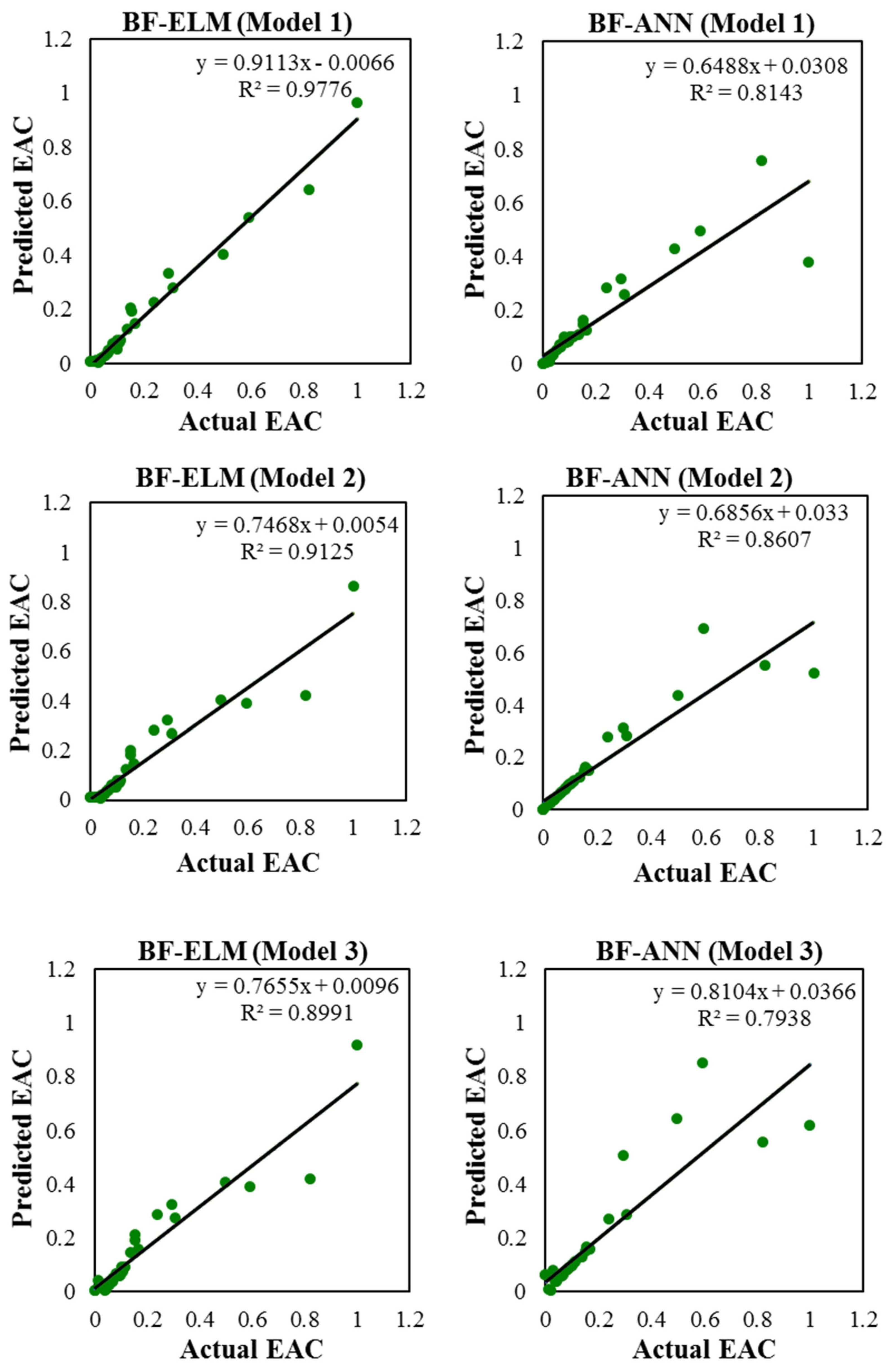
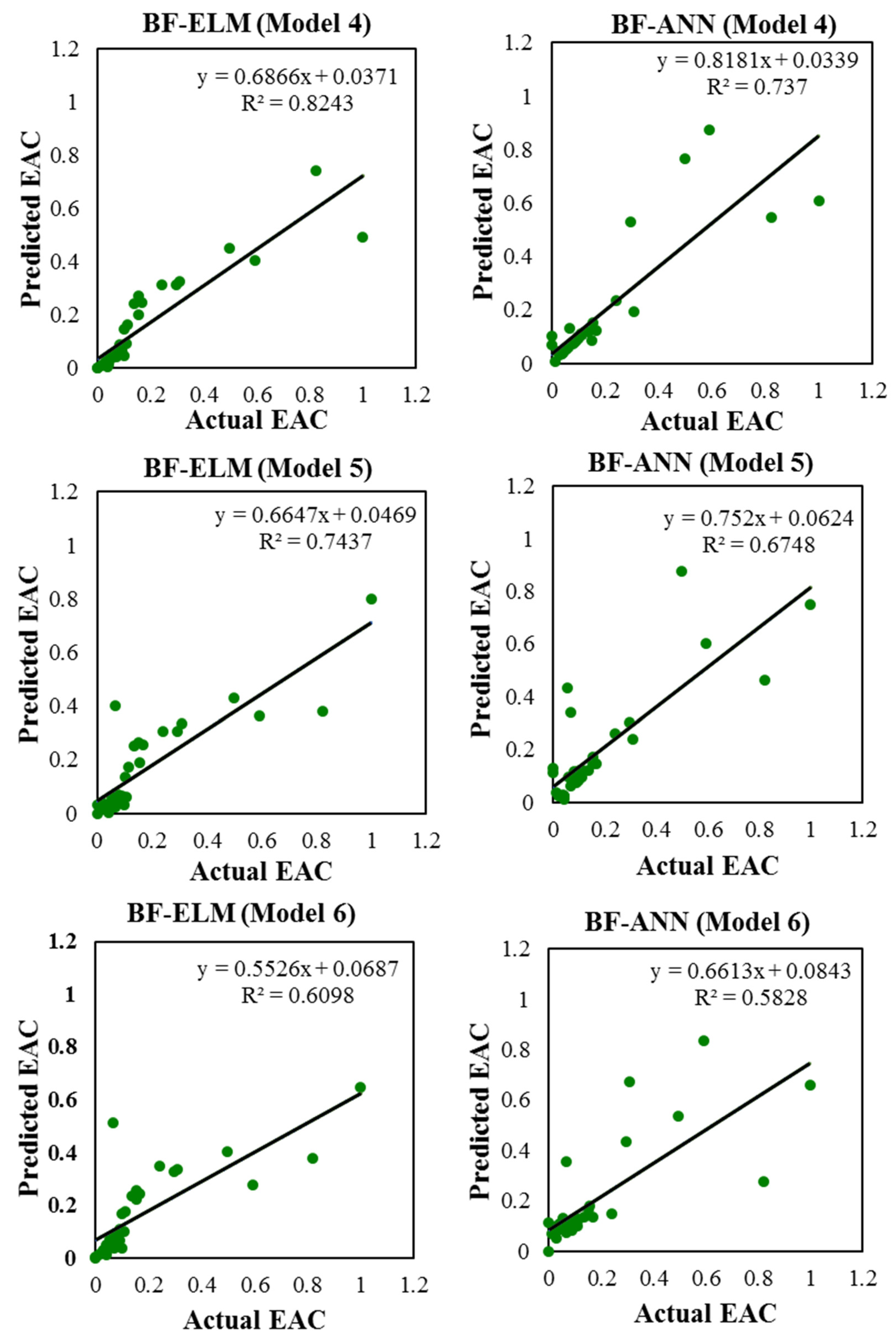
The hybridized BF-ELM model showed a different prediction performance (Table 6 and Table 7) in terms of the 7 input variables (CV, SV, CPI, SPI, Subcontractor billed index, Change order index, and CCI). At its optimal performance, it presented a minimum RMSE value of approximately 0.043 and R approximately 0.98 using only the CV and SV parameters.

The performance of the BF-ELM model was better than that of GHS-ELM model, but it should be noted that the BF-ELM model required more execution time to abstract the internal relationship between the predictors and the predicted. The results of the input combinations variables and the prediction performances of the GHS-ANN are displayed in Table 8 and Table 9, respectively.

The optimum input combination of the GHS-ANN model was performed using the 3rd combination by including the CV, CPI, SPI, and CCI variables. On the other hand, BF-ANN allocates its best predictability using the 2nd input combination by incorporating the CV, SV, and CPI variables. For more convenience, a comparative analysis was performed between the GHS-ELM and GHS-ANN models and the BF-ELM and BF-ANN models. The comparison of the GHS-ELM and GHS-ANN models showed that the GHS-ELM model was superior in terms of significant improvements based on the quantitative measurables. There was a reduction in the RMSE-MAE values by 25.8–23.1%, while the NSE-R values were enhanced by 8–6.2%. This demonstrated the suitability of the GHS-ELM model in establishing the relationship between the project elements and the EAC phenomena.

Another way of evaluation usually used to visualize the predictive models’ capability is scatter plot. The scatter plot or the variation from the best fit line is a graphical way of representing the relationship between actual and predicted values. Figure 3, Figure 4 and Figure 5 showed the deviation from the ideal 45° line for the ELM and ANN, for the GHS-ELM and GHS-ANN, and for the BF-ELM and BF-ANN models, respectively.

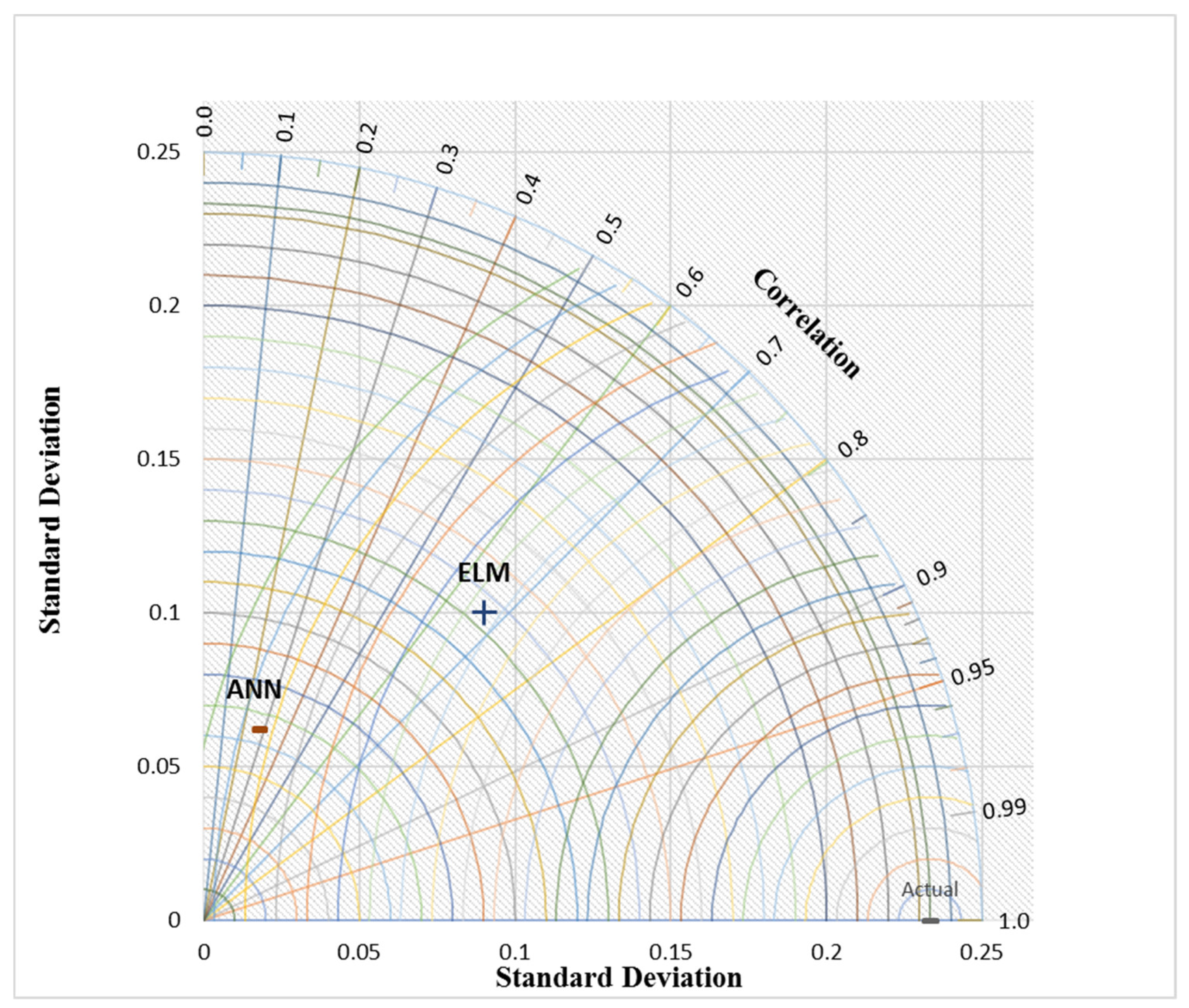
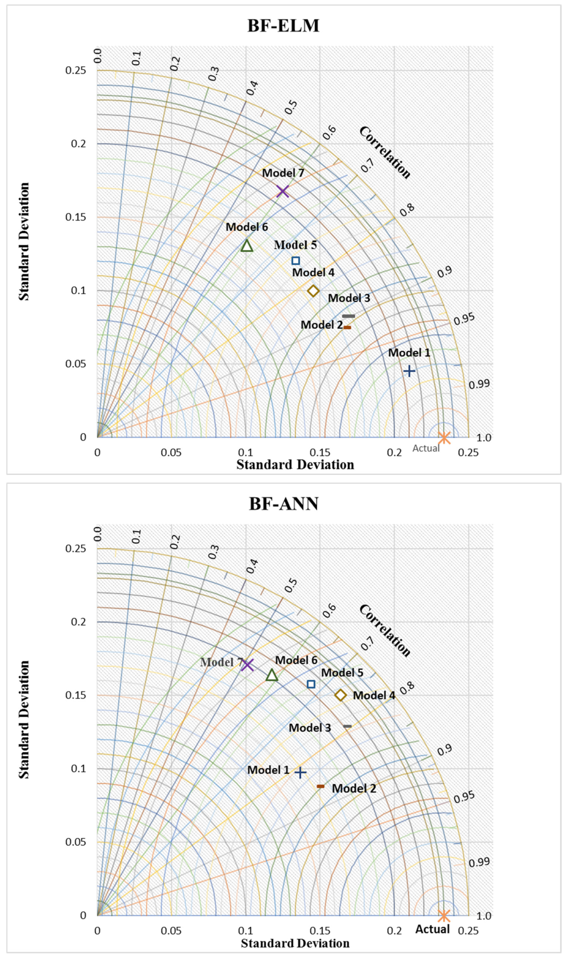
This is evidence of a perfect agreement between the performance of the hybrid intelligent model over the classical one. A graphical representation of the three metrics (standard deviation, correlation, and root mean square error) was presented in Figure 6 (this figure is referred to as the Taylor Diagram).

With this diagram, it is easier to determine the optimal combination of model inputs based on the distance from the observed EAC benchmarking data. As shown in Figure 6, ELM was more accurate compared to ANN in terms of the level of correlation and the standard deviation whereas the hybrid GHS-ELM model showed that Model 2 achieved a closer prediction value to the actual EAC. On the other hand, the GHS-ANN model achieved the best input variables with Model 3. The modeling in general does not show a consistence in the input variability due to the nature of the studied problem. In conclusion, the main contribution of this study is that it highlighted the effectiveness of the hybrid GHS-ELM model which is comprised of the input selection optimizer and ELM as the predictive model. The proposed GHS-ELM is a robust framework which can contribute to the monitoring of engineering project costs by assisting the project managers in monitoring the completion cost of an ongoing project.

4. Conclusions

This research explored a new hybrid data-intelligence predictive model called global harmony search integrated with extreme learning machine which can assist construction managers to reliably control project cost and make accurate EAC predictions. There are two phases performed in this intelligence system; first is the attribute-based variable selection phase where the GHS algorithm was used to determine the related variables that can influence the prediction task, and second is the implementation of the predictive ELM model for the EAC. For reliability purposes, the proposed ELM model was validated against the classical ANN model by performing the same hybridization process for the input selection. Another input selection approach was used to analyze the GHS algorithm in the form of the variable assortment called brute force. In this research, civil construction projects’ information was used to construct the predictive models. Based on the ELM and ANN-based model results, the ELM model achieved better results compared to the classical ANN. However, the incorporation of the input selection algorithm remarkably enhanced the predictability of the ELM model. Furthermore, the predictability of the hybridized intelligent model exhibited more reliable and accurate results. Worth to report, this research can be extended with the possibility of investigating the uncertainty of error that exists in construction project costs.

References

- Zeng, J.; An, M.; Smith, N.J. Application of a fuzzy based decision making methodology to construction project risk assessment. Int. J. Proj. Manag. 2007, 25, 589–600. [Google Scholar] [CrossRef]
- Dvir, D. Transferring projects to their final users: The effect of planning and preparations for commissioning on project success. Int. J. Proj. Manag. 2005, 23, 257–265. [Google Scholar] [CrossRef]
- Cheng, M.Y.; Peng, H.S.; Wu, Y.W.; Chen, T.L. Estimate at completion for construction projects using evolutionary support vector machine inference model. Autom. Constr. 2010, 19, 619–629. [Google Scholar] [CrossRef]
- Anbari, F.T. Earned Value Project Management Method and Extensions. Proj. Manag. J. 2003, 34, 12–23. [Google Scholar] [CrossRef]
- Narbaev, T.; De Marco, A. Combination of Growth Model and Earned Schedule to Forecast Project Cost at Completion. J. Constr. Eng. Manag. 2014, 140, 04013038. [Google Scholar] [CrossRef]
- Vandevoorde, S.; Vanhoucke, M. A comparison of different project duration forecasting methods using earned value metrics. Int. J. Proj. Manag. 2006, 24, 289–302. [Google Scholar] [CrossRef]
- Larson, E.W.; Gray, C.F. A Guide to the Project Management Body of Knowledge—PMBOK Guide; Project Management Institute: Newtown Square, PA, USA, 2004; Volume 3, ISBN 9781935589679. [Google Scholar]
- Christensen, D.S. Determining an accurate estimate at completion. Natl. Contract Manag. J. 1993, 25, 17–25. [Google Scholar]
- Christensen, D.S.; Antolini, R.C.; McKinney, J.W. A Review of Estimate at Completion Research. J. Cost Anal. 1995, 12, 41–62. [Google Scholar] [CrossRef]
- Abu Hammad, A.A.; Ali, S.M.; Sweis, G.J.; Sweis, R.J. Statistical Analysis on the Cost and Duration of Public Building Projects. J. Manag. Eng. 2010. [Google Scholar] [CrossRef]
- Khosrowshahi, F.; Kaka, A.P. Estimation of project total cost and duration for housing projects in the U.K. Build. Environ. 1996. [Google Scholar] [CrossRef]
- Narbaev, T.; De Marco, A. An Earned Schedule-based regression model to improve cost estimate at completion. Int. J. Proj. Manag. 2014, 32, 1007–1018. [Google Scholar] [CrossRef]
- Cheng, M.Y.; Tsai, H.C.; Liu, C.L. Artificial intelligence approaches to achieve strategic control over project cash flows. Autom. Constr. 2009, 18, 386–393. [Google Scholar] [CrossRef]
- Abba, W. Earned value management—Reconciling government and commercial practices. Program Manag. 1997, 26, 58–63. [Google Scholar]
- Vitner, G.; Rozenes, S.; Spraggett, S. Using data envelope analysis to compare project efficiency in a multi-project environment. Int. J. Proj. Manag. 2006, 24, 323–329. [Google Scholar] [CrossRef]
- Leu, S.-S.; Lin, Y.-C. Project Performance Evaluation Based on Statistical Process Control Techniques. J. Constr. Eng. Manag. 2008, 134, 813–819. [Google Scholar] [CrossRef]
- Lipke, W.; Zwikael, O.; Henderson, K.; Anbari, F. Prediction of project outcome. The application of statistical methods to earned value management and earned schedule performance indexes. Int. J. Proj. Manag. 2009, 27, 400–407. [Google Scholar] [CrossRef]
- Plaza, M.; Turetken, O. A model-based DSS for integrating the impact of learning in project control. Decis. Support Syst. 2009, 47, 488–499. [Google Scholar] [CrossRef]
- Pajares, J.; López-Paredes, A. An extension of the EVM analysis for project monitoring: The Cost Control Index and the Schedule Control Index. Int. J. Proj. Manag. 2011. [Google Scholar] [CrossRef]
- Willems, L.L.; Vanhoucke, M. Classification of articles and journals on project control and earned value management. Int. J. Proj. Manag. 2015. [Google Scholar] [CrossRef]
- Abellan-Nebot, J.V.; Subrión, F.R. A review of machining monitoring systems based on artificial intelligence process models. Int. J. Adv. Manuf. Technol. 2009. [Google Scholar] [CrossRef]
- Iranmanesh, S.H.; Zarezadeh, M. Application of artificial neural network to forecast actual cost of a project to improve earned value management system. In Proceedings of the World Congress on Science, Engineering and Technology, Kuala Lumpur, Malaysia, 25–26 March 2008; pp. 240–243. [Google Scholar]
- Cheng, M.Y.; Roy, A.F.V. Evolutionary fuzzy decision model for construction management using support vector machine. Expert Syst. Appl. 2010, 37, 6061–6069. [Google Scholar] [CrossRef]
- Cheng, M.-Y.; Tsai, H.-C.; Sudjono, E. Conceptual cost estimates using evolutionary fuzzy hybrid neural network for projects in construction industry. Expert Syst. Appl. 2010, 37, 4224–4231. [Google Scholar] [CrossRef]
- Cheng, M.Y.; Hoang, N.D.; Roy, A.F.V.; Wu, Y.W. A novel time-depended evolutionary fuzzy SVM inference model for estimating construction project at completion. Eng. Appl. Artif. Intell. 2012, 25, 744–752. [Google Scholar] [CrossRef]
- Feylizadeh, M.R.; Hendalianpour, A.; Bagherpour, M. A fuzzy neural network to estimate at completion costs of construction projects. Int. J. Ind. Eng. Comput. 2012, 3, 477–484. [Google Scholar] [CrossRef]
- Caron, F.; Ruggeri, F.; Merli, A. A bayesian approach to improve estimate at completion in earned value management. Proj. Manag. J. 2013, 44, 3–16. [Google Scholar] [CrossRef]
- Wauters, M.; Vanhoucke, M. Support Vector Machine Regression for project control forecasting. Autom. Constr. 2014, 47, 92–106. [Google Scholar] [CrossRef]
- Golizadeh, H.; Banihashemi, S.; Sadeghifam, A.N.; Preece, C. Automated estimation of completion time for dam projects. Int. J. Constr. Manag. 2017, 17, 197–209. [Google Scholar] [CrossRef]
- Huang, G.-B.; Zhu, Q.-Y.; Siew, C.-K. Extreme learning machine: Theory and applications. Neurocomputing 2006, 70, 489–501. [Google Scholar] [CrossRef]
- Huang, G.; Huang, G.B.; Song, S.; You, K. Trends in extreme learning machines: A review. Neural Netw. 2015, 61, 32–48. [Google Scholar] [CrossRef]
- Yaseen, Z.M.; Sulaiman, S.O.; Deo, R.C.; Chau, K.-W. An enhanced extreme learning machine model for river flow forecasting: State-of-the-art, practical applications in water resource engineering area and future research direction. J. Hydrol. 2018, 569, 387–408. [Google Scholar] [CrossRef]
- Huang, G.-B.; Chen, L. Convex incremental extreme learning machine. Neurocomputing 2007, 70, 3056–3062. [Google Scholar] [CrossRef]
- Avci, E. A new method for expert target recognition system: Genetic wavelet extreme learning machine (GAWELM). Expert Syst. Appl. 2013, 40, 3984–3993. [Google Scholar] [CrossRef]
- Sahin, M.; Kaya, Y.; Uyar, M.; Yildrm, S. Application of extreme learning machine for estimating solar radiation from satellite data. Int. J. Energy Res. 2014, 38, 205–212. [Google Scholar] [CrossRef]
- Shamshirband, S.; Mohammadi, K.; Tong, C.W.; Petkovi, D.; Porcu, E.; Mostafaeipour, A.; Ch, S.; Sedaghat, A. Application of extreme learning machine for estimation of wind speed distribution. Clim. Dyn. 2016, 46, 1893–1907. [Google Scholar] [CrossRef]
- Samat, A.; Du, P.; Member, S.; Liu, S.; Li, J.; Cheng, L. Ensemble Extreme Learning Machines for Hyperspectral Image Classification. IEEE Sel. Top. Appl. Earth Obs. Remote Sens. J. 2014, 7, 1060–1069. [Google Scholar] [CrossRef]
- Soria-Olivas, E.; Gómez-Sanchis, J.; Martín, J.D.; Vila-Francés, J.; Martínez, M.; Magdalena, J.R.; Serrano, A.J. BELM: Bayesian extreme learning machine. IEEE Trans. Neural Netw. 2011, 22, 505–509. [Google Scholar] [CrossRef] [PubMed]
- Bhat, A.U.; Merchant, S.S.; Bhagwat, S.S. Prediction of Melting Points of Organic Compounds Using Extreme Learning Machines. Ind. Eng. Chem. Res. 2008, 47, 920–925. [Google Scholar] [CrossRef]
- Lian, C.; Zeng, Z.; Yao, W.; Tang, H. Displacement prediction model of landslide based on ensemble of extreme learning machine. In Lecture Notes in Computer Science, Proceedings of the International Conference on Neural Information Processing, Doha, Qatar, 12–15 November 2012; Springer: Berlin, Germany, 2012; Volume 7666, pp. 240–247. [Google Scholar] [CrossRef]
- Yaseen, Z.M.; Deo, R.C.; Hilal, A.; Abd, A.M.; Bueno, L.C.; Salcedo-Sanz, S.; Nehdi, M.L. Predicting compressive strength of lightweight foamed concrete using extreme learning machine model. Adv. Eng. Softw. 2018, 115, 112–125. [Google Scholar] [CrossRef]
- Sanikhani, H.; Deo, R.C.; Yaseen, Z.M.; Eray, O.; Kisi, O. Non-tuned data intelligent model for soil temperature estimation: A new approach. Geoderma 2018, 330, 52–64. [Google Scholar] [CrossRef]
- Yaseen, Z.M.; Allawi, M.F.; Yousif, A.A.; Jaafar, O.; Hamzah, F.M.; El-Shafie, A. Non-tuned machine learning approach for hydrological time series forecasting. Neural Comput. Appl. 2016, 30, 1–3. [Google Scholar] [CrossRef]
- Li, J.; Salim, R.D.; Aldlemy, M.S.; Abdullah, J.M.; Yaseen, Z.M. Fiberglass-Reinforced Polyester Composites Fatigue Prediction Using Novel Data-Intelligence Model. Arab. J. Sci. Eng. 2018. [Google Scholar] [CrossRef]
- Hou, M.; Zhang, T.; Weng, F.; Ali, M.; Al-Ansari, N.; Yaseen, Z. Global Solar Radiation Prediction Using Hybrid Online Sequential Extreme Learning Machine Model. Energies 2018, 11, 3415. [Google Scholar] [CrossRef]
- Sanikhani, H.; Deo, R.C.; Samui, P.; Kisi, O.; Mert, C.; Mirabbasi, R.; Gavili, S.; Yaseen, Z.M. Survey of different data-intelligent modeling strategies for forecasting air temperature using geographic information as model predictors. Comput. Electron. Agric. 2018, 152, 242–260. [Google Scholar] [CrossRef]
- Shanmuganathan, S. Artificial Neural Network Modelling. Stud. Comput. Intell. 2016, 628, 1–14. [Google Scholar] [CrossRef]
- Wang, S.-C. Artificial Neural Network; McGraw-Hill: New York, NY, USA, 2003; ISBN 978-1-118-88906-0. [Google Scholar]
- Tino, P.; Benuskova, L.; Sperduti, A. Artificial Neural Network Models; Springer Handbook of Computational Intelligence; Springer: Berlin/Heidelberg, Germany, 2015; ISBN 9783662435052. [Google Scholar]
- Yaseen, Z.M.; El-Shafie, A.; Afan, H.A.; Hameed, M.; Mohtar, W.H.M.W.; Hussain, A. RBFNN versus FFNN for daily river flow forecasting at Johor River, Malaysia. Neural Comput. Appl. 2015. [Google Scholar] [CrossRef]
- Kurt, H.; Kayfeci, M. Prediction of thermal conductivity of ethylene glycol-water solutions by using artificial neural networks. Appl. Energy 2009, 86, 2244–2248. [Google Scholar] [CrossRef]
- Hemmat Esfe, M.; Afrand, M.; Yan, W.-M.; Akbari, M. Applicability of artificial neural network and nonlinear regression to predict thermal conductivity modeling of Al2O3–water nanofluids using experimental data. Int. Commun. Heat Mass Transf. 2015, 66, 246–249. [Google Scholar] [CrossRef]
- Omran, M.G.H.; Mahdavi, M. Global-best harmony search. Appl. Math. Comput. 2008, 198, 643–656. [Google Scholar] [CrossRef]
- Ouyang, H.B.; Gao, L.Q.; Kong, X.Y.; Li, S.; Zou, D.X. Hybrid harmony search particle swarm optimization with global dimension selection. Inf. Sci. 2016, 346–347, 318–337. [Google Scholar] [CrossRef]
- Osborne, A.R. Simple, Brute-force computation of theta functions and beyond. Int. Geophys. 2010, 97, 489–499. [Google Scholar]
- Heule, M.J.H.; Kullmann, O. The Science of Brute Force. Commun. ACM 2017, 60, 70–79. [Google Scholar] [CrossRef]
- Chai, T.; Draxler, R.R. Root mean square error (RMSE) or mean absolute error (MAE)?—Arguments against avoiding RMSE in the literature. Geosci. Model Dev. 2014, 7, 1247–1250. [Google Scholar] [CrossRef]
- Nash, J.E.; Sutcliffe, J.V. River flow forecasting through conceptual models part I—A discussion of principles. J. Hydrol. 1970, 10, 282–290. [Google Scholar] [CrossRef]
- Tao, H.; Diop, L.; Bodian, A.; Djaman, K.; Ndiaye, P.M.; Yaseen, Z.M. Reference evapotranspiration prediction using hybridized fuzzy model with firefly algorithm: Regional case study in Burkina Faso. Agric. Water Manag. 2018, 208, 140–151. [Google Scholar] [CrossRef]
Figure 1.
The proposed global harmony search-extreme learning machine GHS -ELM model for the prediction of the estimation at completion (EAC).
Figure 2.
The input–output systematic structure of the hybrid ELM predictive model.
Figure 3.
The correlation variance between the classical ELM and ANN predictive models over the testing phase.
Figure 4.
The correlation variance between the hybrid GHS-ELM and GHS-ANN predictive models over the testing phase for all the investigated input combinations.
Figure 5.
The correlation variance between the hybrid BF-ELM and BF-ANN predictive models over the testing phase for all the investigated input combinations.
Figure 6.
The Taylor diagram presentations of the proposed hybrid predictive models and the comparable ones.