Abstract
Multiple Input Multiple Output Orthogonal Frequency Division Multiplexing (MIMO-OFDM) proves to be a better choice for high speed underwater acoustic (UWA) communication as it increases the data rate and solves the bandwidth limitation issue; however, at the same time, it increases the design challenges and complexity of the receivers. Inter-Symbol Interference (ISI) and Inter-Carrier Interference (ICI) are introduced in the received signal by the extended multipath and Doppler shifts along with different types of noises due to the noisy acoustic channel. Here we propose two iterative receivers: one is ICI unaware iterative MIMO-OFDM receiver, which uses a novel cost function threshold based soft information decision feedback method. The second one is ICI aware progressive iterative MIMO-OFDM receiver, which adapts and increases the progressions according to the level of ICI present in the received signal, while fully utilizing the soft information from the previous iterations, therefore reducing the complexity. Orthogonal Matching pursuit (OMP) channel estimation, low density parity check (LDPC) decoding and minimum mean square error (MMSE) equalization schemes are exploited by both the receivers. The proposed receivers are analyzed and compared with the standard Alamouti MIMO receiver as a reference and also compared with the non-iterative, basic turbo iterative and non-progressive iterative MIMO receivers. Simulations and experimental results prove the efficiency and effectiveness of the proposed receivers.
1. Introduction
Underwater acoustics (UWA) communication has attracted huge attention during the last two decades because of the extension of its applications to different domains. UWA sensor networks are introduced, which increased the design challenges to meet the higher demands [1]. The challenges like high data rate, low bit error rate (BER), and utilization of maximum channel capacity still have a lot of room for improvement. Underwater communication is no match with the terrestrial wireless communication as the sound speed in water is at least five orders of magnitude less than the speed of wireless radio channels. Therefore, alternate ways need to be found in order to improve the efficiency of UWA communication, as the speed of sound is constant inside water and cannot be increased. Moreover, the acoustic wave propagation speed differs from ocean to ocean depending on numerous factors [2,3].
Channel modeling is the basic step of any communication model, where the effects of the varying channel on the acoustic signal are found out and signal attenuation due to ambient noises, multipath, and Doppler Effect are analyzed. Multipath introduces inter-symbol interference (ISI) and Doppler shift introduces Inter-carrier Interference (ICI) [4,5]. Modulation scheme plays an important role in designing an underwater communication model. No matter how proficient the channel is modeled, without a competent modulation scheme, a reliable and efficient model cannot be designed. Orthogonal Frequency Division Multiplexing (OFDM) is considered to be a low-complexity and highly efficient modulation scheme, which overcomes the problem of ISI to a large extent. OFDM uses multiple carriers, sending some bits on each channel; hence all the sub-channels are dedicated to data source. The carriers are orthogonally spaced in the frequency domain, which helps the demodulator in rejecting frequencies other than its own. The increased symbol duration in OFDM helps in combating ISI. OFDM also has higher data rate and spectral sufficiency, therefore, it becomes the most suitable option for multipath environment [6].
MIMO was introduced recently in UWA communication to efficiently use the acoustic bandwidth and increase the system capacity by exploiting the spatial diversity. The parallel transmission of independent data streams in MIMO improves the data rate performance [7]. The combination of MIMO and OFDM is a tempting low-complexity solution for bandwidth-efficient communications over frequency selective and bandwidth limited UWA channels [8,9,10,11,12].
Channel estimation, equalization, and de-coding are the key steps in designing any receiver, which get the signal back into the proper shape as it was when transmitted. Channel estimation estimates the channel parameters. The channel estimation of MIMO systems is an intricate job, as each received signal consists of independent information from every transmitter and all the channels need to be estimated at the same time [13,14,15]. Equalization removes the effects of the channel on the received signal and removes the ISI, Inter carrier interference (ICI), and other distortions from the signal. Channel coding adds some redundancy in the useful bits in order to protect the data in a noisy channel.
The complexity of the UWA receiver has always been pointed out as the main problem in designing any UWA communication system [16]. Different receivers were designed focusing on the performance and complexity of the receiving system [17,18]. In this paper we propose a low-complexity, novel progressive iterative MIMO-OFDM receiver for the UWA communication system, which outperforms all the previous designs in terms of complexity and performance. The proposed design is compared with another non-iterative receiver, basic Turbo iterative receiver, and also with a Turbo iterative receiver with channel estimation inside the loop.
The rest of the paper is organized as: Section 2 gives a UWA MIMO OFDM system model, Section 3 explains ICI unaware iterative receiver in detail, and Section 4 describes ICI aware progressive iterative receiver. Section 5 gives the simulation and experimental results for both the receivers and Section 6 concludes our work.
2. UWA MIMO-OFDM System Model
Consider a UWA MIMO-OFDM system with transmitters and receivers. The duration of the overall OFDM block is given by , where denotes the OFDM symbol duration and denotes the guard interval. The subcarrier spacing can be given by and for total number of subcarriers, the bandwidth can be given by . For transmit-receive pair in a MIMO system, assume that the acoustic multipath channel consists of discrete paths and the channel impulse response can be calculated as:
where , and show the amplitude of the path of transmit-receive pair, delay at the start of the OFDM block and the Doppler factor corresponding to the path. The fast Fourier transform (FFT) output of the subcarrier of the receiver can be obtained as follows, where shows all the transmitted symbols:
When the system does not have the influence of ICI, (the subscript is omitted here for convenience) is a diagonal matrix; whereas when ICI exists, is a regular matrix and can be written as:
where the element in the vector is the ICI factor, which represents the subcarrier interference with the subcarrier. Generally, is a large matrix and in most channel estimation algorithms, it needs to be inverted, which involves a higher amount of computation. Therefore, in order to decrease the complexity, we reduce to a strip matrix by assuming that each symbol is only interfered by the adjacent symbols, i.e.,
Figure 1 shows a visual illustration of with different values of .
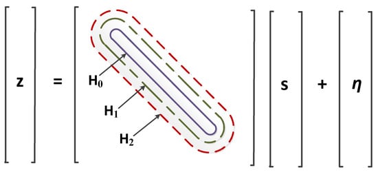
Figure 1.
Channel model with different degrees of Inter-Carrier Interference (ICI).
When D = 0, it indicates that the system has no influence of ICI, that is, all subcarriers of OFDM are orthogonal. Therefore, Equation (2) can be re-written as:
Denote with , Equation (5) can be rewritten in matrix form as:
3. ICI Unaware Cost Function Based Soft Feedback Iterative Receiver
Threshold controlled and uncontrolled soft and hard decision feedback methods are already in practice in iterative receiver systems [19]. The soft symbol estimates are claimed to be better than the hard symbol estimates, especially for iterative channel estimation as they provide more statistical information about the transmitted data [20]. First, we design an iterative receiver which is unaware of ICI and treats ICI as an additive noise as shown in Figure 2. The receiver uses a novel cost based soft decision feedback method which will be explained in detail later.
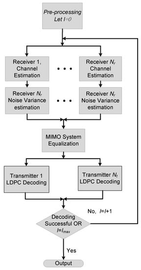
Figure 2.
ICI unaware Multiple Input Multiple Output Orthogonal Frequency Division Multiplexing (MIMO-OFDM) Iterative Receiver block diagram.
The initial processing of MIMO-OFDM iterative receiver is the same as that of a non-iterative receiver processing, i.e., the channel estimation is performed first, then equalization, and finally decoding. OMP sparse estimation, MMSE equalization, and LDPC decoding algorithms are adopted here. The initial channel estimate is obtained from a training sequence contained within the transmitted signal. After the first equalization and decoding of a block of data, the output is fed back to the channel estimator, which then produces a better channel estimate which is passed on to the equalizer and subsequently to the decoder. In the decoding process, if the parity condition is satisfied or the number of iterations reaches the preset maximum value , the algorithm stops and gives us the output.
3.1. OMP Channel Estimation
The OMP algorithm is a kind of greedy algorithm, which first searches the dictionary for elements that match the received signal, orthogonalizes the selected element, removes the effect of the element from the signal and the dictionary, and obtains the signal residual. Then in the remaining dictionary, it continues to search for the element that has the best match with the signal residual, and the above process is repeated until the residual satisfies the set threshold [21]. The following linear model is usually used to analyze the sparse channel estimation problem:
During the channel estimation, shows the received pilot information, is the noise vector, shows the channel information to be estimated and is the constructed dictionary vector as given by:
where shows the elements in the dictionary and represents the amplitudes corresponding to different paths in the channel. Let be the residual after iterations with initial value , search for the elements in the dictionary that have the largest inner product of residuals and get the index of the matching element in the dictionary:
where is the index of the previous iterations. Schmidt orthogonalization of the selected elements is given by:
where is the value of the orthogonalized element chosen for the first time and the estimated values of elements in signal is given by:
and the residual signal is calculated as:
Stop the iterations when (where is the residual threshold). Finally the delay estimation value can be obtained from Equation (7), with being the corresponding path gain, the resulting channel frequency estimate is given by:
where is a diagonal matrix with the diagonal elements satisfying the following equation;
3.2. Cost Function Controlled Soft Information Feedback
Threshold controlled or uncontrolled hard and soft decision feedback methods are normally used in iterative receivers. We propose a new feedback method that uses cost function as a decision condition threshold. Based on the cost function threshold, it decides whether to select the current iterative channel estimation result or to use the pilot-aided initial channel estimation value. This design is based on the idea given in reference [22], where a cost function was used for the decision feedback in a SISO coded OFDM wireless communication system. However, the cost function of the channel estimation for the current iteration was always compared with the initial channel cost function , whereas we compared the cost function of the current iteration with the cost function of the previous iteration of channel estimation . The advantage of this change is that the cost function keeps updating in comparison to the previous iteration, therefore, the performance of the channel estimation improves. Furthermore, in reference [22], pilot-assisted channel estimation was performed based on the hard feedback method. We used soft feedback and OMP channel estimation, which obviously improves the channel estimation performance [23]. This improved decision feedback method based on the cost function is given by:
where indicates the number of iterations, and represent the signal detection cost function and channel estimation cost function for subcarrier, respectively. To derive the cost function , the iterative receiver input is taken from the demodulated received symbols that serves as auxiliary pilots. The modified signal model at the iterative receiver is given by:
where is given by:
The decision feedback induces this additional noise component, that can be approximated as additive white Gaussian noise (AWGN) with a zero mean and its variance is given by:
where is the variance of the AWGN signal and can be generated from the LLR of the decoder output [22].
4. ICI Aware Progressive MIMO-OFDM Iterative Receiver
Studies have shown that there is usually more severe ICI in real time underwater acoustic OFDM systems. Specialized ICI equalization methods can be used to significantly improve system performance instead of considering ICI as an additive noise. The canonical ICI aware iterative receivers assume a constant ICI depth D and the preprocessing procedure is kept unchanged throughout the iterations. When the ICI depth is kept large, it covers the scenarios with large channel variations, however when the channel variation is not that large, the large ICI depth results in over calculations, more power consumption and increased complexity. On the other hand, if ICI depth is assumed small, the performance gets worse for UWA communication with large channel variations.
Since the computationally efficient receiving algorithm is critical to the UWA communication networks, a progressive iterative receiver is designed here which adapts the ICI model according to the unknown channel conditions during iterations. The proposed receiver, as shown in Figure 3, is an iterative receiver which follows the Turbo principle, however, unlike the canonical iterative receivers, the system model used for channel identification and data demodulation changes during each iteration. It starts with a simple channel model i.e., ICI ignorant processing and then proceeds to ICI-aware processing where the severity of the assumed ICI increases as iteration goes on. The soft information obtained from the previous iteration contributes to the channel estimation, equalization, and data demodulation for the current iteration. Moreover, if the decoding of the current iteration is unsuccessful, the system increases the value of in the next iteration, assuming a greater Doppler factor value and therefore more ICI. The increment in value of enhances the equalization effect of the ICI and the value of is gradually increased from 0 with each iteration. Therefore, the receiver can self-adapt to the unknown degree of channel variation progressively. The progressive iterative receiver has a very low complexity under better channel conditions and can even maintain good performance under poor channel conditions as proved in the simulations section.
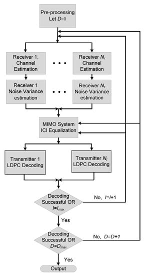
Figure 3.
Progressive MIMO-OFDM iterative receiver block diagram.
ICI Equalization of MIMO System
Based on Equation (5), the FFT outputs of the receivers associated with the transmitted symbols on the subcarrier of all data streams can be written as:
where
The channel matrix of dimensions (2D+1) × (4D+1) can be expressed as:
If the value of is zero, it means there is no ICI in the system and the channel matrix will be a strip matrix having non-zero values only at the diagonals. With the increase in value of , the channel matrix gets complex and the number of non-zero entries increase. The purpose of the MIMO system ICI equalization is to estimate the transmitted information symbol while mitigating the effects of ICI in the system. This paper uses the ICI equalization method based on a priori information (mean and variance) and MMSE criteria [24]. The specific steps are described as follows:
Let the expectation of the transmitter subcarriers be , the variance be , and be the (D+1)th column of the matrix , then
The number of its constituent elements is 2D+1. It is assumed that the matrix removes to obtain the matrix , and the vector removes the element to obtain the vector . To obtain the estimated value of , rewrite equation (19) as:
which can be simplified as:
To estimate , we need to use the information of the adjacent subcarriers of the current data stream and the data symbols that will interfere with the estimated symbols from other data streams . The mean and variance of are:
During the initial iteration of equalization, the mean and variance of are unknown and can be set to 0 and , respectively, i.e., and .
In addition, the equivalent noise is assumed to be Gaussian white noise with a covariance matrix of , where .
Based on Equation (24), the MMSE estimate for is:
where
where is a diagonal matrix with the first elements equal to , followed by next elements equal to and so on.
5. Results
The results section is comprised of two parts: First we discuss and compare the results of ICI unaware iterative receiver and then we discuss the results of the ICI aware progressive iterative receiver for MIMO OFDM communication.
5.1. ICI Unaware Iterative Receiver
5.1.1. Simulation Results
The simulation is based on a MIMO-OFDM system and Bellhop is used to generate the impulse responses of the four-channels. The simulation parameters used are given in Table 1.

Table 1.
MIMO-OFDM simulation parameters.
The proposed iterative receiver is simulated and compared with the non-iterative receiver as well as with the basic turbo iterative receiver with soft information feedback, where the channel estimation is kept outside the iteration loop. Channel estimation is performed after the preprocessing of the data and then the information is iterated between the equalizer and decoder while the channel estimation does not participate in the iterative process. Furthermore, the proposed receiver is also compared with the standard Alamouti MIMO receiver as a reference, using the same data rate and same channel. Figure 4 shows the comparison of BER curves of the standard Alamouti scheme, non-iterative, basic turbo iterative, and the proposed iterative receivers. Figure 4a shows that even the non-iterative MIMO system performance is better than the Alamouti MIMO system performance using the same channel and data rate. The reason is that in the Alamouti design, the transmitted signals from both the transducers are not entirely different, rather one is the complex conjugate of the other, while in the MIMO system, the transmitted signals from both the transmitters are entirely different and independent. Figure 4a further shows that the proposed turbo iterative receiver with channel estimation included in the loop performs better than the basic turbo iterative receiver without the channel estimation in the loop and there is an obvious difference in the performance of the non-iterative receiver. Figure 4b shows that the performance of the proposed iterative receiver improves with each iteration and it gets stable after four iterations.
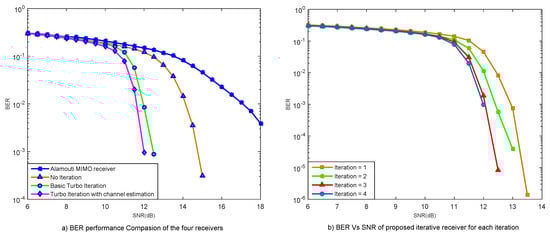
Figure 4.
Bit error rate (BER) simulation performance comparison of the proposed iterative receiver.
5.1.2. Experimental Results
The performance of the iterative reception algorithm in the underwater acoustic MIMO-OFDM communication system is verified by a pool experiment. The experiment was conducted in the pool of Harbin Engineering University, China. The pool is about 45m long, 6m wide, and 5m deep. The transmitting array has 2 transducers. The first transducer is placed around 2m below the water surface and the second one is placed around 3.3m below the water surface. The distance between the two transducers is kept around 1.3m. Due to the high transmission response of the transmitters and the high sensitivity of the receiving hydrophones in the experiment, the signal generator is used to directly send the signal to the transmitters without the use of an amplifier and also the received signal is collected directly. There are two vertical arrays, A and B, at the receiving side, each having 14 hydrophones. The acquisition channel sequence is such that the receiving vertical array A receives 114 channels, while vertical array B receives 15-28 channels.
Each data frame contains 8 OFDM symbols, QPSK mapping is adopted and the coding method is 1/2 code rate LDPC code. Combining the received data of different hydrophones of the vertical arrays A and B, the greater the number of combined channels, the greater the signal to noise ratio, thereby improving the processing performance. Select the 2nd, 4th, 6th, 11th, 16th, 18th, 19th, 20th, and 25th receive hydrophones orderly to receive signals in 10 frames per sequence. We compared the performance of the basic turbo iterative receiver with the channel estimation outside the loop and the proposed iterative receiver with channel estimation inside the loop by combining a different number of hydrophones, as shown in Figure 5. It can be seen that in the basic turbo receiver, the iterative processing does not improve the performance of the system and the BER increases when 6 and 7 hydrophones are combined. The BER is even worse than the case where the non-iterative receiver was used. The reason behind this is that the initial channel estimation may have large errors in this experiment, resulting in poor performance for the iterative receivers that do not include channel estimation. Part (b) of the Figure 5 shows the BER performance of the proposed iterative receiver with the increase in the number of hydrophones for each iteration, and it can be seen that as the number of iterations increases, the system performance is significantly improved, and the performance tends to get stable after three iterations. Furthermore, if we increase the number of merged hydrophones for data collection, the effect of the iterative reception algorithm gets more obvious.
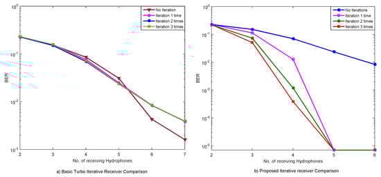
Figure 5.
Experimental results comparison of the two receivers.
5.2. ICI Aware Progressive Iterative Receiver
5.2.1. Simulation Results
Adding the effect of the non-uniform Doppler to the four channels of a 2 X 2 MIMO-OFDM system, while using the same simulation parameters as used above. The system was tested in good channel conditions as well as poor channel conditions and it was assumed that the Doppler factor of each path obeyed the uniform distribution with zero mean value and the standard deviations of the relative motion speeds of sending and receiving ends were set to and and the corresponding maximum Doppler shift factors are , respectively. The Doppler factor step length is set to .
First, we analyze the influence of the value of D on the ICI equalization effect of non-progressive MIMO-OFDM iterative receiver shown in Figure 6. Figure 6a shows that for , when D is set to 0, the system performance is poor. When D is set to 1, the system performance is significantly improved. The value of D is continuously increased; however, the trend of further improvement in the system performance is not obvious. This shows that even when there is a slight ICI in the MIMO-OFDM system, it cannot be ignored as it will also have a significant impact on BER performance. Therefore in such cases, we can just take value of D = 1 for the ICI equalization.
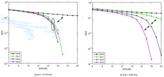
Figure 6.
BER performance of non-progressive iterative MIMO receiver with different values of D and σv.
For , similarly if the ICI is not equalized (D = 0), the system performance is poor. With each increase in the value of D, an obvious improvement can be observed as highlighted by the arrows in the Figure 6b, indicating that when there is a more serious ICI in the system, the value of D can be increased accordingly to equalize the ICI.
Figure 6 also shows that if we assume the value of D = 2 in the case, the non-progressive system will stop the iterations while the system will still have a lot of ICI left to be equalized. Similarly if the D is taken as 3 in case, the non-progressive receiver will keep iterating unnecessarily and will increase the complexity.
Next, the progressive iterative reception algorithm for MIMO-OFDM systems considering ICI is simulated. Assuming , the number of Doppler factors corresponding to D = 1, 2, and 3 in the iteration process is taken as 6, 10, and 14, respectively. D = 1 iterates 2 times, thus it actually runs 5 times in total. The BER performance at various values of the iterative MIMO-OFDM progressive iterative receiver is shown in Figure 7. It can be seen from Figure 7 that the progressive iterative receiving algorithm can significantly improve the system performance for a MIMO-OFDM system with ICI. As the iteration progresses, the value of D gradually increases and the BER of the system gradually decreases, which verifies the effectiveness of the progressive MIMO-OFDM iterative receiver.
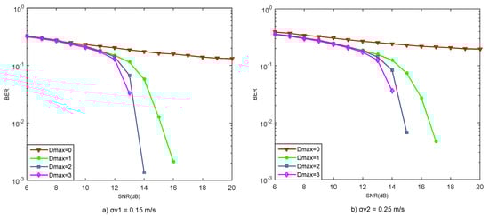
Figure 7.
BER performance of progressive MIMO-OFDM iterative receivers with different values of D and σv.
Figure 8 compares the performance of the non-progressive iterative receiver and progressive iterative receiver for σv = 0.25. Initially when the D and Dmax both are 0, i.e., there is no ICI equalization, both the curves are the same. Later on, the performance of the progressive receiver after the fourth progression is compared with the performance of the non-progressive receiver with D = 3; and it can be observed that the performance of the progressive iterative receiver is better than that of non-progressive iterative receiver.
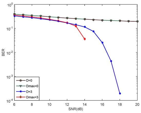
Figure 8.
Comparison of the MIMO progressive and non-progressive iterative receivers.
Now we further compare the complexity of the two iterative receivers, which we claim to be the main advantage of the proposed model. Based on the time spent in computer simulation, the complexity is compared in Figure 9. The simulation is performed using the computer, with Intel(R) Core(TM) i7-7700 CPU@3.60GHz 3.60GHz processor and the MATLAB version 2015a used. Corresponding to each signal-to-noise ratio, the average running time of multiple cycles of an OFDM symbol is plotted for the fourth iterations of both receivers, i.e., D = 3 and Dmax = 3. It can be seen that progressive iterative receiver has significantly less runtime, which leads to the conclusion that progressive iterative receiver has lower complexity as compared to non-progressive iterative receiver.

Figure 9.
Comparison of complexity of MIMO progressive and non-progressive receivers.
5.2.2. Experimental Results
In order to verify the effectiveness of the proposed MIMO-OFDM ICI-aware progressive iterative receiver, this section tests the system experimentally by adding Doppler to the experimental setup discussed in Section 5.1.2. The Doppler is added manually to the system by moving the transmitters, while keeping all other conditions unchanged. The 10 received signals of the 2nd, 3rd, 5th, 10th and 8th receiving hydrophones are sequentially combined to test the proposed MIMO-OFDM progressive iterative receiving algorithm. In the iterative process, the values of the Doppler factor corresponding to are taken as 6 and 10 respectively, where is iterated twice, therefore it is actually iterated three times in total. The BER values for different number of combined receiving hydrophones and different value of are given in Table 2. The table also compares the BER performance with the BER values of the ICI-unaware receiver BER for .
Table 2.
BER comparison of iterative MIMO-OFDM receiver for different number of combined hydrophones in pool experiment.
Table 2 shows that as the iterative process progresses, the value of increases gradually and the performance of the system is significantly improved, which proves the effectiveness of the progressive iterative receiver. At the same time, it can be seen that the BER values of the ICI-unaware receiver when iterated three times is very close to the BER values of the ICI-aware receiver after third progression. The reason behind this may be the smaller Doppler shift, which results in less ICI and therefore can be ignored in the actual processing.
Furthermore, using the CP-based UWA Doppler scaling factor estimation method [25], the Doppler scaling factor is sequentially estimated for eight OFDM symbols in one frame of different receiving hydrophones, as shown in Figure 10. It can be seen that the Doppler scaling factor is in the order of 10−5, which confirms that the Doppler shift is really small. This may be due to the slow speed of the movement of the array by hand, as the transmitting array is relatively heavy and might not be disturbed properly, therefore, causing a smaller Doppler scaling factor. In this case, it is recommended to use the ICI-unaware iterative receiving algorithm, because of its closer performance to the ICI-aware progressive receiving algorithm with fewer processing and calculations.
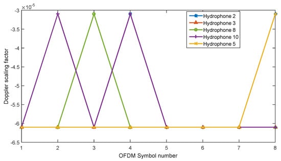
Figure 10.
Doppler scaling factor estimation values for different hydrophones for eight OFDM symbols in one frame.
6. Conclusions
This paper proposes two types of iterative receivers for MIMO-OFDM UWA communication systems. The first one is an ICI unaware iterative receiver, which uses soft information decision feedback based on a novel cost function threshold method. The receiver exploits the OMP channel estimation and LDPC coding scheme for MIMO-OFDM communication. The receiver is tested and compared with the non-iterative receiver as well as basic Turbo Iterative receiver with soft information feedback, where the channel estimation is kept outside the iteration loop. Simulations and experimental results prove the effectiveness of the proposed receiver.
Secondly, we propose an ICI aware progressive iterative MIMO-OFDM receiver, which equalizes the ICI and adapts the ICI model according to the unknown channel conditions during the iterations. The value of D is progressively increased according to the level of the ICI present in the signal. The proposed receiver is compared with the non-progressive iterative receiver and its effectiveness is proved through simulations and pool experiment. Furthermore, both the receivers were compared in terms of complexity and an obvious reduction in complexity is noticed by the proposed progressive iterative receiver while equalizing the same level of ICI.
Author Contributions
Conceptualization, G.Q. and Z.B.; methodology, L.M. and F.Z.; software, X.L.; validation, L.M. and Z.B.; formal analysis, X.L.; investigation, L.M.; resources, G.Q. and F.Z.; data curation, Z.B. and X.L.; writing—original draft preparation, Z.B.; writing—review and editing, L.M.; visualization, X.L.; supervision, G.Q.; project administration, G.Q.; funding acquisition, G.Q.
Funding
This research was supported by the National Natural Science Foundation of China under Grants 61431004, 61601136, 61601137, and 61771152, and the Fundamental Research Funds for the Central Universities of China under Grants HEUCF180501.
Conflicts of Interest
The authors declare no conflict of interest.
References
- Ullah, U.; Khan, A.; Altowaijri, M.S.; Ali, I.; Rahman, U.A.; Kumar, V.; Ali, M.; Mahmood, H. Cooperative and Delay Minimization Routing Schemes for Dense Underwater Wireless Sensor Networks. Symmetry 2019, 11, 195. [Google Scholar] [CrossRef]
- Palou, G.; Stojanovic, M. Underwater acoustic MIMO OFDM: An experimental analysis. In Proceedings of the OCEANS 2009, Biloxi, MS, USA, 26–29 October 2009. [Google Scholar]
- Xu, Y.; Xue, W.; Li, Y.; Guo, L.; Shang, W. Multiple Signal Classification Algorithm Based Electric Dipole Source Localization Method in an Underwater Environment. Symmetry 2017, 9, 231. [Google Scholar] [CrossRef]
- Mason, S.; Berger, C.; Zhou, S.; Ball, K.; Freitag, L.; Willett, P. An OFDM Design for Underwater Acoustic Channels with Doppler Spread. In Proceedings of the Digital Signal Processing Workshop and 5th IEEE Signal Processing Education Workshop (DSP/SPE 2009), Marco Island, FL, USA, 4–7 January 2009. [Google Scholar]
- Beheshti, M.; Omidi, M.J.; Doost-Hoseini, A.M. Joint ICI and IBI cancelation for underwater acoustic MIMO-OFDM systems. In Proceedings of the 2011 19th Iranian Conference on Electrical Engineering, Tehran, Iran, 17–19 May 2011. [Google Scholar]
- Li, B.; Huang, J.; Zhou, S.; Ball, K.; Stojanovic, M.; Freitag, L.; Willett, P. MIMO-OFDM for High-Rate Underwater Acoustic Communications. IEEE J. Ocean. Eng. 2009, 34, 634–644. [Google Scholar]
- Yu, H.; Yang, G.; Meng, F.; Li, Y. Performance Analysis of MIMO System with Single RF Link Based on Switched Parasitic Antenna. Symmetry 2017, 9, 304. [Google Scholar] [CrossRef]
- Stojanovic, M. Low Complexity OFDM Detector for Underwater Acoustic Channels. In Proceedings of the OCEANS 2006, Boston, MA, USA, 18–21 September 2006. [Google Scholar]
- Ormondroyd, R.F. A Robust Underwater Acoustic Communication System using OFDM-MIMO. In Proceedings of the OCEANS 2007—Europe, Aberdeen, UK, 18–21 June 2007. [Google Scholar]
- Carrascosa, P.C.; Stojanovic, M. Adaptive Channel Estimation and Data Detection for Underwater Acoustic MIMO—OFDM Systems. IEEE J. Ocean. Eng. 2010, 35, 635–646. [Google Scholar] [CrossRef]
- Bouvet, P.J.; Loussert, A. Capacity analysis of underwater acoustic MIMO communications. In Proceedings of the 2010 IEEE OCEANS, Sydney, Australia, 24–27 May 2010. [Google Scholar]
- Yu, H.; Yang, G.; Li, Y.; Meng, F. Design and Analysis of Multiple-Input Multiple-Output Radar System Based on RF Single-Link Technology. Symmetry 2018, 10, 130. [Google Scholar] [CrossRef]
- Yang, G.; Yin, J.; Huang, D.; Jin, L.; Zhou, H. A Kalman Filter-Based Blind Adaptive Multi-User Detection Algorithm for Underwater Acoustic Networks. IEEE Sens. J. 2016, 16, 4023–4033. [Google Scholar] [CrossRef]
- Shahjehan, W.; Shah, W.S.; Lloret, J.; Leon, A. A Low Rank Channel Estimation Scheme in Massive Multiple-Input Multiple-Output. Symmetry 2018, 10, 507. [Google Scholar] [CrossRef]
- Jung, Y.-A.; You, Y.-H. Efficient Joint Estimation of Carrier Frequency and Sampling Frequency Offsets for MIMO-OFDM ATSC Systems. Symmetry 2018, 10, 554. [Google Scholar] [CrossRef]
- Huang, J.; Zhou, S.; Wang, Z. Performance Results of Two Iterative Receivers for Distributed MIMO OFDM With Large Doppler Deviations. IEEE J. Ocean. Eng. 2013, 38, 347–357. [Google Scholar] [CrossRef]
- Xuandi, S.; Zhe, J.; Xiaohong, S.; Xin, W. A computational-efficient turbo receiver for mobile underwater acoustic channels. In Proceedings of the 2017 IEEE International Conference on Signal Processing, Communications and Computing (ICSPCC), Xiamen, China, 22–25 October 2017. [Google Scholar]
- Banerjee, S.; Agrawal, M.; Fauziya, F. A Generalized Gaussian noise receiver for improved underwater communication in leptokurtic noise. In Proceedings of the OCEANS 2017, Aberdeen, UK, 19–22 June 2017. [Google Scholar]
- Niu, H.; Ritcey, J.A. Iterative channel estimation and decoding of pilot symbol assisted LDPC coded QAM over flat fading channels. In Proceedings of the Thrity-Seventh Asilomar Conference on Signals, Systems & Computers, Pacific Grove, CA, USA, 9–12 November 2003. [Google Scholar]
- Laot, C.; Glavieux, A.; Labat, J. Turbo equalization: Adaptive equalization and channel decoding jointly optimized. IEEE J. Sel. Areas Commun. 2001, 19, 1744–1752. [Google Scholar] [CrossRef]
- Berger, C.R.; Zhou, S.; Preisig, J.C.; Willett, P. Sparse Channel Estimation for Multicarrier Underwater Acoustic Communication: From Subspace Methods to Compressed Sensing. IEEE Trans. Signal Process. 2010, 58, 1708–1721. [Google Scholar] [CrossRef]
- Auer, G.; Bonnet, J. Threshold Controlled Iterative Channel Estimation for Coded OFDM. In Proceedings of the 2007 IEEE 65th Vehicular Technology Conference—VTC2007-Spring, Dublin, Ireland, 22–25 April 2007. [Google Scholar]
- Qiao, G.; Babar, Z.; Ma, L.; Liu, S.; Wu, J. MIMO-OFDM underwater acoustic communication systems—A review. Phys. Commun. 2017, 23, 56–64. [Google Scholar] [CrossRef]
- Tuchler, M.; Singer, A.C.; Koetter, R. Minimum mean squared error equalization using a priori information. IEEE Trans. Signal Process. 2002, 50, 673–683. [Google Scholar] [CrossRef]
- Ma, L.; Qiao, G.; Liu, S. A Combined Doppler Scale Estimation Scheme for Underwater Acoustic OFDM System. J. Comput. Acoust. 2015, 23, 1540004. [Google Scholar] [CrossRef]
© 2019 by the authors. Licensee MDPI, Basel, Switzerland. This article is an open access article distributed under the terms and conditions of the Creative Commons Attribution (CC BY) license (http://creativecommons.org/licenses/by/4.0/).