The Logic of Pseudo-Uninorms and Their Residua

Abstract

Our method for density elimination is generalized to the non-commutative substructural logic ${\mathbf{GpsUL}}^{*}$. Then, the standard completeness of ${\mathbf{HpsUL}}^{*}$ follows as a lemma by virtue of previous work by Metcalfe and Montagna. This result shows that ${\mathbf{HpsUL}}^{*}$ is the logic of pseudo-uninorms and their residua and answered the question posed by Prof. Metcalfe, Olivetti, Gabbay and Tsinakis.

1. Introduction

Prof. Metcalfe, Olivetti and Gabbay conjectured that the Hilbert system $\mathbf{HpsUL}$ is the logic of pseudo-uninorms and their residua in 2009 in [1]. It is not the case, as shown by Prof. Wang and Zhao in [2], although $\mathbf{HpsUL}$ is the logic of bounded representable residuated lattices. We constructed the system ${\mathbf{HpsUL}}^{*}$ by adding the weakly commutativity rule

$$(WCM)⊢(A⇝t)\to (A\to t)$$

to $\mathbf{HpsUL}$ and conjectured that it is the logic of residuated pseudo-uninorms and their residua in 2013 in [3].

In this paper, we prove the conjecture by showing that the density elimination holds for the hypersequent system ${\mathbf{GpsUL}}^{*}$ corresponding to ${\mathbf{HpsUL}}^{*}$. Then, the standard completeness of ${\mathbf{HpsUL}}^{*}$ follows as a lemma by virtue of previous work by Metcalfe and Montagna [4]. That is, ${\mathbf{HpsUL}}^{*}$ is complete with respect to algebras whose lattice reduct is the real unit interval $[0,1]$. Thus, ${\mathbf{HpsUL}}^{*}$ is a kind of substructural fuzzy logic [4], and potentially has certain applications to fuzzy inferences and expert Systems [5,6,7,8]. Our result also shows that that ${\mathbf{HpsUL}}^{*}$ is an axiomatization for the variety of residuated lattices generated by all dense residuated chains. Thus, we have also answered the question posed by Prof. Metcalfe and Tsinakis in [9] in 2017.

In proving the density elimination for ${\mathbf{GpsUL}}^{*}$, we have to overcome several difficulties as follows. Firstly, cut-elimination doesn’t holds for ${\mathbf{GpsUL}}^{*}$. Note that $(WCM)$ and the density rule $(D)$ are formulated as

$$\frac{G|\Gamma ,\Delta \Rightarrow t}{G|\Delta ,\Gamma \Rightarrow t},\frac{G|\Pi \Rightarrow p|\Gamma ,p,\Delta \Rightarrow B}{G|\Gamma ,\Pi ,\Delta \Rightarrow B}$$

in ${\mathbf{GpsUL}}^{*}$, respectively. Consider the following derivation fragment.

By the induction hypothesis of the proof of cut-elimination, we get that $G_1|G_2|{\Gamma }_1,{\Gamma }_2,{\Delta }_2,{\Delta }_1\Rightarrow A$ from $G_2|{\Gamma }_2,{\Delta }_2\Rightarrow t$ and $G_1|{\Gamma }_1,t,{\Delta }_1\Rightarrow A$ by $(CUT)$. However, we can’t deduce $G_1|G_2|{\Gamma }_1,{\Delta }_2,{\Gamma }_2,{\Delta }_1\Rightarrow A$ from $G_1|G_2|{\Gamma }_1,{\Gamma }_2,{\Delta }_2,{\Delta }_1\Rightarrow A$ by $(WCM)$. We overcome this difficulty by introducing the following weakly cut rule into ${\mathbf{GpsUL}}^{*}$

$$\frac{G_1|\Gamma ,t,\Delta \Rightarrow A{G}_2|\Pi \Rightarrow t}{G_1|G_2|\Gamma ,\Pi ,\Delta \Rightarrow A}(WCT).$$

Secondly, the proof of the density elimination for ${\mathbf{GpsUL}}^{*}$ becomes troublesome even for some simple cases in $\mathbf{GUL}$ [4]. Consider the following derivation fragment

Here, the major problem is how to extend $(D)$ such that it is applicable to $G_2|{\Gamma }_2,{\Pi }_2^{\prime },p,{\Pi }_2^{″},{\Sigma }_2\Rightarrow p$. By replacing p with t, we get $G_2|{\Gamma }_2,{\Pi }_2^{\prime },t,{\Pi }_2^{″},{\Sigma }_2\Rightarrow t$. However, there exists no derivation of $G_1|G_2|{\Gamma }_1,{\Pi }_2^{\prime },{\Gamma }_2,{\Pi }_1,{\Sigma }_2,{\Pi }_2^{″},{\Sigma }_1\Rightarrow A_1$ from $G_2|{\Gamma }_2,{\Pi }_2^{\prime },{\Pi }_2^{″},{\Sigma }_2\Rightarrow t$ and $G_1|{\Gamma }_1,{\Pi }_1,{\Sigma }_1\Rightarrow A_1$. Notice that ${\Gamma }_2,{\Pi }_2^{\prime }$ and ${\Pi }_2^{″},{\Sigma }_2$ in $G_2|{\Gamma }_2,{\Pi }_2^{\prime },p,{\Pi }_2^{″},{\Sigma }_2\Rightarrow p$ are commutated simultaneously in $G_1|G_2|{\Gamma }_1,{\Pi }_2^{\prime },{\Gamma }_2,{\Pi }_1,{\Sigma }_2,{\Pi }_2^{″},{\Sigma }_1\Rightarrow A_1$, which we can’t obtain by $(WCM)$. It seems that $(WCM)$ can’t be strengthened further in order to solve this difficulty. We overcome this difficulty by introducing a restricted subsystem ${\mathbf{GpsUL}}_{\Omega }$ of ${\mathbf{GpsUL}}^{*}$. ${\mathbf{GpsUL}}_{\Omega }$ is a generalization of ${\mathbf{GIUL}}_{\Omega }$, which we introduced in [10] in order to solve a longstanding open problem, i.e., the standard completeness of $\mathbf{IUL}$. Two new manipulations, which we call the derivation-splitting operation and derivation-splicing operation, are introduced in ${\mathbf{GpsUL}}_{\Omega }$.

The third difficulty we encounter is that the conditions of applying the restricted external contraction rule $(E{C}_{\Omega })$ become more complex in ${\mathbf{GpsUL}}_{\Omega }$ because new derivation-splitting operations make the conclusion of the generalized density rule to be a set of hypersequents rather than one hypersequent. We continue to apply derivation-grafting operations in the separation algorithm of the multiple branches of ${\mathbf{GIUL}}_{\Omega }$ in [10], but we have to introduce a new construction method for ${\mathbf{GpsUL}}_{\Omega }$ by induction on the height of the complete set of maximal $(pEC)$-nodes rather than on the number of branches.

The structure of this paper is as follows. In Section 2, we present two hypersequent calculi ${\mathbf{GpsUL}}^{*}$ and ${\mathbf{GpsUL}}_{\Omega }$, and prove that Cut-elimination does not hold for ${\mathbf{GpsUL}}^{*}$. Because of the absence of the commutativity rule, we have to introduce two novel operations, i.e., the derivation-splitting operation and derivation-splicing operation, in ${\mathbf{GpsUL}}_{\Omega }$ in Section 3, and then we present a suitable definition of the generalized density rule $(\mathcal{D})$ for ${\mathbf{GpsUL}}_{\mathbf{\Omega }}$. In Section 4, we adapt the old main algorithm in the system ${\mathbf{GIUL}}_{\mathbf{\Omega }}$ to the new system ${\mathbf{GpsUL}}_{\mathbf{\Omega }}$. In Section 5, we propose two directions for future research.

2. $\mathbf{GpsUL}$, ${\mathbf{GpsUL}}^{*}$ and ${\mathbf{GpsUL}}_{\Omega }$

Definition 1. 

([1]) $\mathbf{GpsUL}$ consists of the following initial sequents and rules:

Initial sequents

$$\frac{}{A\Rightarrow A}(ID)\frac{}{\Rightarrow t}(t_r)\frac{}{\Gamma ,\perp ,\Delta \Rightarrow A}({\perp }_l)\frac{}{\Gamma \Rightarrow \top }({\top }_r),$$

Structural Rules

$$\frac{G|\Gamma \Rightarrow A|\Gamma \Rightarrow A}{G|\Gamma \Rightarrow A}(EC)\frac{G}{G|\Gamma \Rightarrow A}(EW),$$

$$\frac{G_1|{\Gamma }_1,{\Pi }_1,{\Delta }_1\Rightarrow A_1{G}_2|{\Gamma }_2,{\Pi }_2,{\Delta }_2\Rightarrow A_2}{G_1|G_2|{\Gamma }_1,{\Pi }_2,{\Delta }_1\Rightarrow A_1|{\Gamma }_2,{\Pi }_1,{\Delta }_2\Rightarrow A_2}(COM),$$

Logical Rules

$$\begin{array}{cc}\begin{array}{c}\hfill \frac{G_1|\Gamma \Rightarrow A{G}_2|\Delta \Rightarrow B}{G_1|G_2|\Gamma ,\Delta \Rightarrow A\odot B}({\odot }_r)\\ \hfill \frac{G_1|\Gamma ,B,\Delta \Rightarrow C{G}_2|\Pi \Rightarrow A}{G_1|G_2|\Gamma ,\Pi ,A\to B,\Delta \Rightarrow C}({\to }_l)\\ \hfill \frac{G_1|\Pi \Rightarrow A{G}_2|\Gamma ,B,\Delta \Rightarrow C}{G_1|G_2|\Gamma ,A⇝B,\Pi ,\Delta \Rightarrow C}({⇝}_l)\\ \hfill \frac{G_1|\Gamma ,A,\Delta \Rightarrow C{G}_2|\Gamma ,B,\Delta \Rightarrow C}{G_1|G_2|\Gamma ,A\vee B,\Delta \Rightarrow C}({\vee }_l)\\ \hfill \frac{G_1|\Gamma \Rightarrow A{G}_2|\Gamma \Rightarrow B}{G_1|G_2|\Gamma \Rightarrow A\wedge B}({\wedge }_l)\\ \hfill \frac{G|\Gamma ,A,\Delta \Rightarrow C}{G|\Gamma ,A\wedge B,\Delta \Rightarrow C}({\wedge }_{rr})\\ \hfill \frac{G|\Gamma ,\Delta \Rightarrow A}{G|\Gamma ,t,\Delta \Rightarrow A}(t_l)\end{array}& \begin{array}{c}\hfill \frac{G|\Gamma ,A,B,\Delta \Rightarrow C}{G|\Gamma ,A\odot B,\Delta \Rightarrow C}({\odot }_l)\\ \hfill \frac{G|A,\Gamma \Rightarrow B}{G|\Gamma \Rightarrow A\to B}({\to }_r)\\ \hfill \frac{G|\Gamma ,A\Rightarrow B}{G|\Gamma \Rightarrow A⇝B}({⇝}_r)\\ \hfill \frac{G|\Gamma \Rightarrow A}{G|\Gamma \Rightarrow A\vee B}({\vee }_{rr})\\ \hfill \frac{G|\Gamma \Rightarrow B}{G|\Gamma \Rightarrow A\vee B}({\vee }_{rl})\\ \hfill \frac{G|\Gamma ,B,\Delta \Rightarrow C}{G|\Gamma ,A\wedge B,\Delta \Rightarrow C}({\wedge }_{rl}).\end{array}\end{array}$$

Cut Rule

$$\frac{G_1|\Gamma ,A,\Delta \Rightarrow B{G}_2|\Pi \Rightarrow A}{G_1|G_2|\Gamma ,\Pi ,\Delta \Rightarrow B}(CUT).$$

Definition 2. 

([3]) ${\mathbf{GpsUL}}^{*}$ is $\mathbf{GpsUL}$ plus the weakly commutativity rule

$$\frac{G|\Gamma ,\Delta \Rightarrow t}{G|\Delta ,\Gamma \Rightarrow t}(WCM).$$

Definition 3.

${\mathbf{GpsUL}}^{*D}$ is ${\mathbf{GpsUL}}^{*}$ plus the density rule $\frac{G|\Pi \Rightarrow p|\Gamma ,p,\Delta \Rightarrow B}{G|\Gamma ,\Pi ,\Delta \Rightarrow B}(D)$.

Lemma 1.

$G\equiv B\vee ((D\to B)\odot C\odot (C\to D)\odot A\to A)$ is not a theorem in $\mathbf{HpsUL}$.

Proof. 

Let $\mathcal{A}={(\{0,1,2,3\},\wedge ,\vee ,\odot ,\to ,⇝,2,0,3)}_{}$ be an algebra, where $x\wedge y=min(x,y)$, $x\vee y=max(x,y)$ for all $x,y\in \{0,1,2,3\}$, and the binary operations ⊙, → and ⇝ are defined by the following tables (see [2]).

By easy calculation, we get that $\mathcal{A}$ is a linearly ordered $\mathbf{HpsUL}$-algebra, where 0 and 3 are the least and the greatest element of $\mathcal{A}$, respectively, and 2 is its unit. Let $v(A)=v(B)=v(C)=v(D)=1$. Then, $v(G)=1\vee (3\odot 1\odot 3\odot 1\to 1)=1<2$. Hence, G is not a tautology in $\mathbf{HpsUL}$. Therefore, it is not a theorem in $\mathbf{HpsUL}$ by Theorem 9.27 in [1]. □

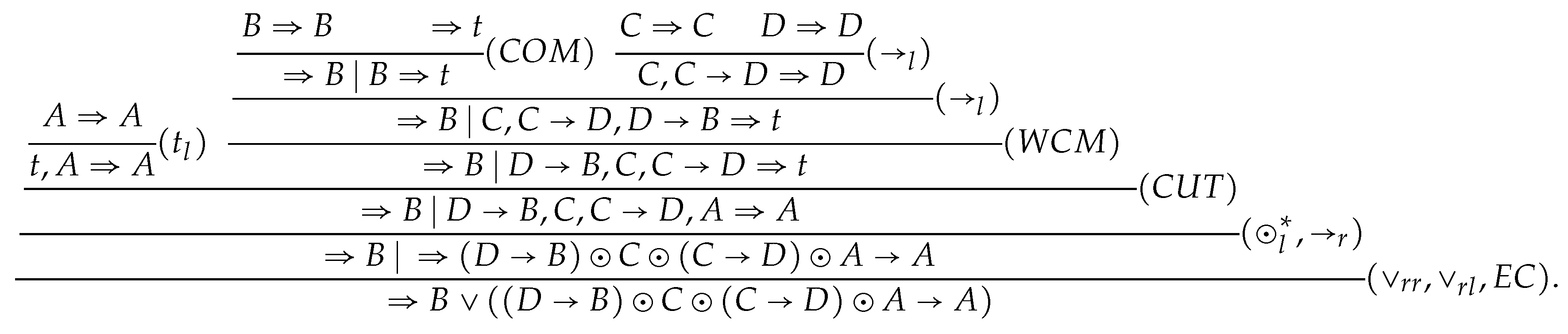
Theorem 1.

Cut-elimination doesn’t hold for ${\mathbf{GpsUL}}^{*}$.

Proof. 

$G\equiv \Rightarrow B\vee ((D\to B)\odot C\odot (C\to D)\odot A\to A)$ is provable in ${\mathbf{GpsUL}}^{*}$, as shown in Figure 1.

Suppose that G has a cut-free proof $\rho$. Then, there exists no occurrence of t in $\rho$ by its subformula property. Thus, there exists no application of $(WCM)$ in $\rho$. Hence, G is a theorem of $\mathbf{GpsUL}$, which contradicts Lemma 1. □

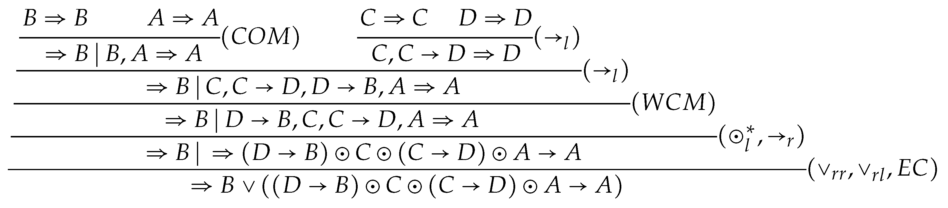
Remark 1.

Following the construction given in the proof of Theorem 53 in [4], $(CUT)$ in Figure 1 is eliminated by the following derivation, as shown in Figure 2. However, the application of $(WCM)$ in ρ is invalid, which illustrates the reason why the cut-elimination theorem doesn’t hold in ${\mathbf{GpsUL}}^{*}$.

Definition 4.

${\mathbf{GpsUL}}^{**}$ is constructed by replacing $(CUT)$ in ${\mathbf{GpsUL}}^{*}$ with

$$\frac{G_1|\Gamma ,t,\Delta \Rightarrow A{G}_2|\Pi \Rightarrow t}{G_1|G_2|\Gamma ,\Pi ,\Delta \Rightarrow A}(WCT).$$

We call it the weakly cut rule and denote it by $(WCT)$.

Theorem 2.

If ${⊢}_{{\mathbf{GpsUL}}^{*}}G$, then ${⊢}_{{\mathbf{GpsUL}}^{**}}G$.

Proof. 

It is proved by a procedure similar to that of Theorem 53 in [4] and omitted. □

Definition 5. 

( [10]) ${\mathbf{GpsUL}}_{\Omega }$ is a restricted subsystem of ${\mathbf{GpsUL}}^{*}$ such that

(i) p is designated as the unique eigenvariable by which we mean that it is not used to build up any formula containing logical connectives and is only used as a sequent-formula.

(ii) Each occurrence of p in a hypersequent is assigned one unique identification number i in ${\mathbf{GpsUL}}_{\Omega }$ and written as $p_i$. Initial sequent $p\Rightarrow p$ of ${\mathbf{GpsUL}}^{*}$ has the form $p_i\Rightarrow p_i$ in ${\mathbf{GpsUL}}_{\Omega }$. p doesn’t occur in $A,\Gamma$ or Δ for each initial sequent $\Gamma ,\perp ,\Delta \Rightarrow A$ or $\Gamma \Rightarrow \top$ in ${\mathbf{GpsUL}}_{\Omega }$.

(iii) Each sequent S of the form ${\Gamma }_0,p,{\Gamma }_1,\cdots ,{\Gamma }_{\lambda -1},p,{\Gamma }_{\lambda }\Rightarrow A$ in ${\mathbf{GpsUL}}^{*}$ has the form ${\Gamma }_0,p_{i_1},{\Gamma }_1,\cdots ,{\Gamma }_{\lambda -1},p_{i_{\lambda }},{\Gamma }_{\lambda }\Rightarrow A$ in ${\mathbf{GpsUL}}_{\Omega }$, where p does not occur in ${\Gamma }_k$ for all $0⩽k⩽\lambda$ and, $i_k\ne i_l$ for all $1⩽k<l⩽\lambda$. Define $v_l(S)=\{i_1,\cdots ,i_{\lambda }\}$, $v_r(S)=\{j_1\}$ if A is an eigenvariable with the identification number $j_1$ and, $v_r(S)=\varnothing$ if A isn’t an eigenvariable.

Let G be a hypersequent of ${\mathbf{GpsUL}}_{\Omega }$ in the form $S_1|\cdots |S_n$ then $v_l(S_k)\bigcap v_l(S_l)=\varnothing$ and $v_r(S_k)\bigcap v_r(S_l)=\varnothing$ for all $1⩽k<l⩽n$. Define $v_l(G)={\bigcup }_{k=1}^n{v}_l(S_k)$, $v_r(G)={\bigcup }_{k=1}^n{v}_r(S_k)$.

(iv) A hypersequent G of ${\mathbf{GpsUL}}_{\Omega }$ is called closed if $v_l(G)=v_r(G)$. Two hypersequents $G^{\prime }$ and $G^{″}$ of ${\mathbf{GpsUL}}_{\Omega }$ are called disjoint if $v_l(G^{\prime })\bigcap v_l(G^{″})=\varnothing$, $v_l(G^{\prime })\bigcap v_r(G^{″})=\varnothing$, $v_r(G^{\prime })\bigcap v_l(G^{″})=\varnothing$ and $v_r(G^{\prime })\bigcap v_r(G^{″})=\varnothing$. $G^{″}$ is a copy of $G^{\prime }$ if they are disjoint and there exist two bijections ${\sigma }_l:v_l(G^{\prime })\to v_l(G^{″})$ and ${\sigma }_r:v_r(G^{\prime })\to v_r(G^{″})$ such that $G^{″}$ can be obtained by applying ${\sigma }_l$ to antecedents of sequents in $G^{\prime }$ and ${\sigma }_r$ to succedents of sequents in $G^{\prime }$.

(v) A hypersequent $G|G_1|G_2$ can be contracted as $G|G_1$ in ${\mathbf{GpsUL}}_{\Omega }$ under certain conditions given in Construction 3, which we called the constraint external contraction rule and denote by $\frac{G^{\prime }|G_1|G_2}{G^{\prime }|G_1}(E{C}_{\Omega })$.

(vi) $(EW)$ is forbidden in ${\mathbf{GpsUL}}_{\Omega }$ and $(EC)$ and $(CUT)$ are replaced with $(E{C}_{\Omega })$ and $(WCT)$, respectively.

(vii) Two rules $({\wedge }_r)$ and $({\vee }_l)$ of $\mathbf{GL}$ are replaced with $\frac{G_1|{\Gamma }_1\Rightarrow A{G}_2|{\Gamma }_2\Rightarrow B}{G_1|G_2|{\Gamma }_1\Rightarrow A\wedge B|{\Gamma }_2\Rightarrow A\wedge B}({\wedge }_{rw})$ and $\frac{G_1|{\Gamma }_1,A,{\Delta }_1\Rightarrow C_1{G}_2|{\Gamma }_2,B,{\Delta }_2\Rightarrow C_2}{G_1|G_2|{\Gamma }_1,A\vee B,{\Delta }_1\Rightarrow C_1|{\Gamma }_2,A\vee B,{\Delta }_2\Rightarrow C_2}({\vee }_{lw})$ in ${\mathbf{GpsUL}}_{\Omega }$, respectively.

(viii) $G_1|S_1$ and $G_2|S_2$ are closed and disjoint for each two-premise inference rule $\frac{G_1|S_1{G}_2|S_2}{G_1|G_2|H^{\prime }}(II)$ of ${\mathbf{GpsUL}}_{\Omega }$ and, $G^{\prime }|S^{\prime }$ is closed for each one-premise inference rule $\frac{G^{\prime }|S^{\prime }}{G^{\prime }|S^{″}}(I)$.

Proposition 1.

Let $\frac{G^{\prime }|S^{\prime }}{G^{\prime }|S^{″}}(I)$ and $\frac{G_1|S_1{G}_2|S_2}{G_1|G_2|H^{\prime }}(II)$ be inference rules of ${\mathbf{GpsUL}}_{\Omega }.$ Then, $v_l(G^{\prime }|S^{″})=v_r(G^{\prime }|S^{″})=v_r(G^{\prime }|S^{\prime })=v_l(G^{\prime }|S^{\prime })$ and $v_l(G_1|G_2|H^{\prime })=v_l(G_1|S_1)\bigcup v_l(G_2|S_2)=$ $v_r(G_1|G_2|H^{\prime })=v_r(G_1|S_1)\bigcup v_r(G_2|S_2)$.

Proof. 

Although $(WCT)$ makes t’s in its premises disappear in its conclusion; it has no effect on identification numbers of the eigenvariable p in a hypersequent because t is a constant in ${\mathbf{GpsUL}}_{\Omega }$ and is distinguished from propositional variables. □

Definition 6.

Let G be a closed hypersequent of ${\mathbf{GpsUL}}_{\Omega }$ and $S\in G$. ${[S]}_G:=\bigcap \{H:S\in H\subseteq G,v_l(H)=v_r(H)\}$ is called a minimal closed unit of G.

3. The Generalized Density Rule $(\mathcal{D})$ for ${\mathbf{GpsUL}}_{\mathbf{\Omega }}$

In this section, ${\mathbf{GL}}_{\mathbf{\Omega }}^{\mathbf{cf}}$ is ${\mathbf{G}}_{\mathbf{ps}}{\mathbf{UL}}_{\Omega }$ without $(E{C}_{\Omega })$. Generally, $A,B,C,\cdots$, denote a formula other than an eigenvariable $p_i$.

Construction 1.Given a proof ${\tau }^{*}$ of $H\equiv G|\Gamma ,p_j,\Delta \Rightarrow p_j$ in ${\mathbf{GL}}_{\mathbf{\Omega }}^{\mathbf{cf}}$, let $T{h}_{{\tau }^{*}}(p_j\Rightarrow p_j)=\left(H_0,\cdots ,H_n\right)$, where $H_0\equiv p_j\Rightarrow p_j$, $H_n\equiv H$. By ${\Gamma }_k,p_j,{\Delta }_k\Rightarrow p_j$, we denote the sequent containing $p_j$ in $H_k$. Then, ${\Gamma }_0=\varnothing$, ${\Delta }_0=\varnothing$, ${\Gamma }_n=\Gamma$ and ${\Delta }_n=\Delta$. Hypersequents ${〈H_k〉}_j^{-}$, ${〈H_k〉}_j^{+}$ and their proofs ${\langle {\tau }^{*}\rangle }_j^{-}\left({〈H_k〉}_j^{-}\right)$, ${\langle {\tau }^{*}\rangle }_j^{+}\left({〈H_k〉}_j^{+}\right)$ are constructed inductively for all $0⩽k⩽n$ in the following such that ${\Gamma }_k\Rightarrow t\in {〈H_k〉}_j^{-}$, ${\Delta }_k\Rightarrow t\in {〈H_k〉}_j^{+}$, and ${〈H_k〉}_j^{+}\setminus \{{\Delta }_k\Rightarrow t\}|{〈H_k〉}_j^{-}\setminus \{{\Gamma }_k\Rightarrow t\}=H_k\setminus \{{\Gamma }_k,p_j,{\Delta }_k\Rightarrow p_j\}$.

(i) ${〈H_0〉}_j^{-}:={〈H_0〉}_j^{+}:=\Rightarrow t$, ${\langle {\tau }^{*}\rangle }_j^{-}\left({〈H_0〉}_j^{-}\right)$ and ${\langle {\tau }^{*}\rangle }_j^{+}\left({〈H_0〉}_j^{+}\right)$ are built up with $\Rightarrow t$.

(ii) Let $\frac{G^{\prime }|S^{\prime }{G}^{″}|S^{″}}{G^{\prime }|G^{″}|H^{\prime }}(II)$ (or $\frac{G^{\prime }|S^{\prime }}{G^{\prime }|S^{″}}(I))$ be in ${\tau }^{*}$, $H_k=G^{\prime }|S^{\prime }$ and $H_{k+1}=G^{\prime }|G^{″}|H^{\prime }$ (accordingly $H_{k+1}=G^{\prime }|S^{″}$ for $(I))$ for some $0⩽k⩽n-1$. There are three cases to be considered.

Case 1. 

$S^{\prime }={\Gamma }_k,p_j,{\Delta }_k\Rightarrow p_j$. If all focus formula(s) of $S^{\prime }$ is (are) contained in ${\Gamma }_k$,

$${〈H_{k+1}〉}_j^{-}:=\left({〈H_k〉}_j^{-}\setminus \{{\Gamma }_k\Rightarrow t\}\right)|G^{″}|H^{\prime }\setminus \{{\Gamma }_{k+1},p_j,{\Delta }_{k+1}\Rightarrow p_j\}|{\Gamma }_{k+1}\Rightarrow t$$

$${〈H_{k+1}〉}_j^{+}:={〈H_k〉}_j^{+}$$

(accordingly ${〈H_{k+1}〉}_j^{-}={〈H_k〉}_j^{-}\setminus \{{\Gamma }_k\Rightarrow t\}|{\Gamma }_{k+1}\Rightarrow t$ for $(I)$) and, ${\langle {\tau }^{*}\rangle }_j^{-}\left({〈H_{k+1}〉}_j^{-}\right)$ is constructed by combining the derivation ${\langle {\tau }^{*}\rangle }_j^{-}\left({〈H_k〉}_j^{-}\right)$ and $\frac{{〈H_k〉}_j^{-}{G}^{″}|S^{″}}{{〈H_{k+1}〉}_j^{-}}(II)$ (accordingly $\frac{{〈H_k〉}_j^{-}}{{〈H_{k+1}〉}_j^{-}}(I)$ for $(I))$ and, ${\langle {\tau }^{*}\rangle }_j^{+}\left({〈H_{k+1}〉}_j^{+}\right)$ is constructed by combining ${\langle {\tau }^{*}\rangle }_j^{+}\left({〈H_k〉}_j^{+}\right)$ and $\frac{{〈H_k〉}_j^{+}}{{〈H_{k+1}〉}_j^{+}}(I{D}_{\Omega })$. The case of all focus formula(s) of $S^{\prime }$ contained in ${\Delta }_k$ is dealt with by a procedure dual to above and omitted.

Case 2. 

$S^{\prime }\in {〈H_k〉}_j^{-}$. ${〈H_{k+1}〉}_j^{-}:=\left({〈H_k〉}_j^{-}\setminus \{S^{\prime }\}\right)|G^{″}|H^{\prime }$ (accordingly ${〈H_{k+1}〉}_j^{-}={〈H_k〉}_j^{-}\setminus \{S^{\prime }\}|S^{″}$ for $(I))$, ${〈H_{k+1}〉}_j^{+}:={〈H_k〉}_j^{+}$ and ${\langle {\tau }^{*}\rangle }_j^{-}\left({〈H_{k+1}〉}_j^{-}\right)$ is constructed by combining the derivation ${\langle {\tau }^{*}\rangle }_j^{-}\left({〈H_k〉}_j^{-}\right)$ and $\frac{{〈H_k〉}_j^{-}{G}^{″}|S^{″}}{{〈H_{k+1}〉}_j^{-}}(II)$ (accordingly $\frac{{〈H_k〉}_j^{-}}{{〈H_{k+1}〉}_j^{-}}(I)$ for $(I))$ and, ${\langle {\tau }^{*}\rangle }_j^{+}\left({〈H_{k+1}〉}_j^{+}\right)$ is constructed by combining ${\langle {\tau }^{*}\rangle }_j^{+}\left({〈H_k〉}_j^{+}\right)$ and $\frac{{〈H_k〉}_j^{+}}{{〈H_{k+1}〉}_j^{+}}(I{D}_{\Omega })$.

Case 3. 

$S^{\prime }\in {〈H_k〉}_j^{+}$. It is dealt with by a procedure dual to Case 2 and omitted.

Definition 7.

The manipulation described in Construction 1 is called the derivation-splitting operation when it is applied to a derivation and the splitting operation when applied to a hypersequent.

Corollary 1.

Let ${⊢}_{{\mathbf{GL}}_{\mathbf{\Omega }}^{\mathbf{cf}}}G|\Gamma ,p_1,\Delta \Rightarrow p_1$. Then, there exist two hypersequents $G_1$ and $G_2$ such that $G=G_1\bigcup G_2$, $G_1\bigcap G_2=\varnothing$, ${⊢}_{{\mathbf{GL}}_{\mathbf{\Omega }}^{\mathbf{cf}}}{G}_1|\Gamma \Rightarrow t$ and ${⊢}_{{\mathbf{GL}}_{\mathbf{\Omega }}^{\mathbf{cf}}}{G}_2|\Delta \Rightarrow t$.

Construction 2. 

Given a proof ${\tau }^{*}$ of $H\equiv G|\Pi \Rightarrow p_j|\Gamma ,p_j,\Delta \Rightarrow A$ in ${\mathbf{GL}}_{\mathbf{\Omega }}^{\mathbf{cf}}$, let $T{h}_{{\tau }^{*}}(p_j\Rightarrow p_j)=(H_0,\cdots ,H_n)$, where $H_0\equiv p_j\Rightarrow p_j$ and $H_n\equiv H$. Then, there exists $1⩽m⩽n$ such that $H_m$ is in the form $G^{\prime }|{\Pi }^{\prime }\Rightarrow p_j|{\Gamma }^{\prime },p_j,{\Delta }^{\prime }\Rightarrow A^{\prime }$ and $H_{m-1}$ is in the form $G^{″}|{\Gamma }^{″},p_j,{\Delta }^{″}\Rightarrow p_j$. A proof of $G|\Gamma ,\Pi ,\Delta \Rightarrow A$ in ${\mathbf{GL}}_{\mathbf{\Omega }}^{\mathbf{cf}}$ is constructed by induction on $n-m$ as follows:

• For the base step, let $n-m=0$. Then, $\frac{H_{n-1}\equiv G^{\prime }|{\Pi }^{\prime },{\Gamma }^{\prime },p_j,{\Delta }^{\prime },{\Pi }^{‴}\Rightarrow p_j{G}^{″}|{\Gamma }^{″},{\Pi }^{″},{\Delta }^{″}\Rightarrow A}{H_n\equiv G^{\prime }|G^{″}|{\Pi }^{\prime },{\Pi }^{″},{\Pi }^{‴}\Rightarrow p_j|{\Gamma }^{″},{\Gamma }^{\prime },p_j,{\Delta }^{\prime },{\Delta }^{″}\Rightarrow A}(COM)\in {\tau }^{*}$, where $G^{\prime }|G^{″}=G$ and ${\Pi }^{\prime },{\Pi }^{″},{\Pi }^{‴}=\Pi$ and ${\Gamma }^{″},{\Gamma }^{\prime }=\Gamma$ and ${\Delta }^{\prime },{\Delta }^{″}=\Delta$. It follows from Corollary 1 that there exist $G_1^{\prime }$ and $G_2^{\prime }$ such that $G^{\prime }=G_1^{\prime }\bigcup G_2^{\prime }$, $G_1^{\prime }\bigcap G_2^{\prime }=\varnothing$, ${⊢}_{{\mathbf{GL}}_{\mathbf{\Omega }}^{\mathbf{cf}}}{G}_1^{\prime }|{\Pi }^{\prime },{\Gamma }^{\prime }\Rightarrow t$ and ${⊢}_{{\mathbf{GL}}_{\mathbf{\Omega }}^{\mathbf{cf}}}{G}_2^{\prime }|{\Delta }^{\prime },{\Pi }^{‴}\Rightarrow t$. Then, $G|\Gamma ,\Pi ,\Delta \Rightarrow A$ is proved as follows:

  $$\begin{array}{|c|}\hline \frac{\frac{\frac{\frac{G^{″}|{\Gamma }^{″},{\Pi }^{″},{\Delta }^{″}\Rightarrow A}{G^{″}|{\Gamma }^{″},t,{\Pi }^{″},{\Delta }^{″}\Rightarrow A}(t_l)\frac{G_1^{\prime }|{\Pi }^{\prime },{\Gamma }^{\prime }\Rightarrow t}{G_1^{\prime }|{\Gamma }^{\prime },{\Pi }^{\prime }\Rightarrow t}(WCM)}{G^{″}|G_1^{\prime }|{\Gamma }^{″},{\Gamma }^{\prime },{\Pi }^{\prime },{\Pi }^{″},{\Delta }^{″}\Rightarrow A}(WCT)}{G^{″}|G_1^{\prime }|{\Gamma }^{″},{\Gamma }^{\prime },{\Pi }^{\prime },{\Pi }^{″},t,{\Delta }^{″}\Rightarrow A}(t_l)\frac{G_2^{\prime }|{\Delta }^{\prime },{\Pi }^{‴}\Rightarrow t}{G_2^{\prime }|{\Pi }^{‴},{\Delta }^{\prime }\Rightarrow t}(WCM)}{G^{″}|G_1^{\prime }|G_2^{\prime }|{\Gamma }^{″},{\Gamma }^{\prime },{\Pi }^{\prime },{\Pi }^{″},{\Pi }^{‴},{\Delta }^{\prime },{\Delta }^{″}\Rightarrow A}(WCT)\\ \hline\end{array}.$$
• For the induction step, let $n-m>0$. Then, it is treated using applications of the induction hypothesis to the premise followed by an application of the relevant rule. For example, let $\frac{H_{n-1}=G^{\prime }|\Pi \Rightarrow p_j|{\Sigma }^{\prime },{\Gamma }^{″},p_j,{\Delta }^{″},{\Sigma }^{‴}\Rightarrow A^{\prime }{G}^{″}|{\Gamma }^{\prime },{\Sigma }^{″},{\Delta }^{\prime }\Rightarrow A}{H_n=G^{\prime }|\Pi \Rightarrow p_j|{\Sigma }^{\prime },{\Sigma }^{″},{\Sigma }^{‴}\Rightarrow A^{\prime }|G^{″}|{\Gamma }^{\prime },{\Gamma }^{″},p_j,{\Delta }^{″},{\Delta }^{\prime }\Rightarrow A}(COM)\in {\tau }^{*}$, where $G^{\prime }|G^{″}|{\Sigma }^{\prime },{\Sigma }^{″},{\Sigma }^{‴}\Rightarrow A^{\prime }=G$ and ${\Gamma }^{\prime },{\Gamma }^{″}=\Gamma$ and ${\Delta }^{″},{\Delta }^{\prime }=\Delta$. By the induction hypothesis, we obtain a derivation of $G|\Gamma ,\Pi ,\Delta \Rightarrow A$:

  $$\frac{G^{\prime }|{\Sigma }^{\prime },{\Gamma }^{″},\Pi ,{\Delta }^{″},{\Sigma }^{‴}\Rightarrow A^{\prime }{G}^{″}|{\Gamma }^{\prime },{\Sigma }^{″},{\Delta }^{\prime }\Rightarrow A}{G^{\prime }|{\Sigma }^{\prime },{\Sigma }^{″},{\Sigma }^{‴}\Rightarrow A^{\prime }|G^{″}|{\Gamma }^{\prime },{\Gamma }^{″},\Pi ,{\Delta }^{″},{\Delta }^{\prime }\Rightarrow A}(COM).$$

Definition 8.

The manipulation described in Construction 2 is called the derivation-splicing operation when it is applied to a derivation and the splicing operation when applied to a hypersequent.

Corollary 2.

If ${⊢}_{{\mathbf{GL}}_{\mathbf{\Omega }}^{\mathbf{cf}}}G|\Pi \Rightarrow p_j|\Gamma ,p_j,\Delta \Rightarrow A$, then ${⊢}_{{\mathbf{GL}}_{\mathbf{\Omega }}^{\mathbf{cf}}}G|\Gamma ,\Pi ,\Delta \Rightarrow A$.

Definition 9. 

(i) Let ${⊢}_{{\mathbf{GL}}_{\mathbf{\Omega }}^{\mathbf{cf}}}H\equiv G|\Gamma ,p_j,\Delta \Rightarrow p_j$. Define ${〈H〉}_j^{-}=G_1|\Gamma \Rightarrow t$, ${〈H〉}_j^{+}=G_2|\Delta \Rightarrow t$ and $D_j(H)=\{G_1|\Gamma \Rightarrow t,G_2|\Delta \Rightarrow t\}$, where $G_1$ and $G_2$ are determined by Corollary 1.

(ii) Let ${⊢}_{{\mathbf{GL}}_{\mathbf{\Omega }}^{\mathbf{cf}}}H\equiv G|\Pi \Rightarrow p_j|\Gamma ,p_j,\Delta \Rightarrow A$. Define $D_j(H)=\{G|\Gamma ,\Pi ,\Delta \Rightarrow A\}={〈H〉}_j$.

(iii) Let ${⊢}_{{\mathbf{GL}}_{\mathbf{\Omega }}^{\mathbf{cf}}}G$. $D_j(G)=\{G\}$ if $p_j$ does not occur in G.

(iv) Let ${⊢}_{{\mathbf{GL}}_{\mathbf{\Omega }}^{\mathbf{cf}}}{G}_i$ for all $1⩽i⩽n$. Define $D_j(\{G_1,\cdots ,G_n\})=D_j(G_1)\bigcup \cdots \bigcup D_j(G_n)$.

(v) Let ${⊢}_{{\mathbf{GL}}_{\mathbf{\Omega }}^{\mathbf{cf}}}G$ and $K=\{1,\cdots ,n\}\subseteq v(G)$. Define $D_K(G)=D_n(\cdots D_2(D_1(G))\cdots )$. Especially, define $\mathcal{D}(G)=D_{v_l(G)}(G)$.

Theorem 3.

Let ${⊢}_{{\mathbf{GL}}_{\mathbf{\Omega }}^{\mathbf{cf}}}G$. Then, ${⊢}_{{\mathbf{GL}}_{\mathbf{\Omega }}^{\mathbf{cf}}}H$ for all $H\in \mathcal{D}(G)$.

Proof. 

Immediately from Corollaries 1, 2 and Definition 9. □

Lemma 2.

Let $G^{\prime }$ be a minimal closed unit of $G|G^{\prime }$. Then, $G^{\prime }$ has the form $\Gamma \Rightarrow A|{\Gamma }_{i_2}\Rightarrow p_{i_2}|\cdots |{\Gamma }_{i_n}\Rightarrow p_{i_n}$ if there exists one sequent $\Gamma \Rightarrow A\in G^{\prime }$ such that A is not an eigenvariable otherwise $G^{\prime }$ has the form ${\Gamma }_{i_1}\Rightarrow p_{i_1}|\cdots |{\Gamma }_{i_n}\Rightarrow p_{i_n}$.

Proof. 

Define $G_1=\Gamma \Rightarrow A$ in Construction 5.2 in [10]. Then, $\varnothing =v_r(G_1)\subseteq v_l(G_1)$. Suppose that $G_k$ is constructed such that $v_r(G_k)\subseteq v_l(G_k)$. If $v_l(G_k)=v_r(G_k)$, the procedure terminates and $n:=k$; otherwise, $v_l(G_k)\setminus v_r(G_k)\ne \varnothing$ and define $i_{k+1}$ to be an identification number in $v_l(G_k)\setminus v_r(G_k)$. Then, there exists ${\Gamma }_{i_{k+1}}\Rightarrow p_{i_{k+1}}\in G\setminus G_k$ by $v_l(G)=v_r(G)$ and define $G_{k+1}=G_k|{\Gamma }_{i_{k+1}}\Rightarrow p_{i_{k+1}}.$ Thus, $v_r(G_{k+1})=v_r(G_k)\bigcup \{i_{k+1}\}\subseteq v_l(G_k)\subseteq v_l(G_{k+1})$. Hence, there exists a sequence $i_2,\cdots ,i_n$ of identification numberssuch that $v_r(G_k)\subseteq v_l(G_k)$ for all $1⩽k⩽n$, where $G_1=\Gamma \Rightarrow A$, $G_k=\Gamma \Rightarrow A|{\Gamma }_{i_2}\Rightarrow p_{i_2}|\cdots |{\Gamma }_{i_k}\Rightarrow p_{i_k}$ for all $2⩽k⩽n$. Therefore, $G^{\prime }$ has the form $\Gamma \Rightarrow A|{\Gamma }_{i_2}\Rightarrow p_{i_2}|\cdots |{\Gamma }_{i_n}\Rightarrow p_{i_n}$. □

Definition 10.

Let $G^{\prime }$ be a minimal closed unit of $G|G^{\prime }$. $G^{\prime }$ is a splicing unit if it has the form $\Gamma \Rightarrow A|{\Gamma }_{i_2}\Rightarrow p_{i_2}|\cdots |{\Gamma }_{i_n}\Rightarrow p_{i_n}$. $G^{\prime }$ is a splitting unit if it has the form ${\Gamma }_{i_1}\Rightarrow p_{i_1}|\cdots |{\Gamma }_{i_n}\Rightarrow p_{i_n}$.

Lemma 3.

Let $G^{\prime }$ be a splicing unit of $G|G^{\prime }$ in the form $\Gamma \Rightarrow A|{\Gamma }_{i_2}\Rightarrow p_{i_2}|\cdots |{\Gamma }_{i_n}\Rightarrow p_{i_n}$ and $K=\{i_2,\cdots ,i_n\}$. Then, $\left|D_K(G|G^{\prime })\right|=1$.

Proof. 

By the construction in the proof of Lemma 2, $i_k\in v_l(G_{k-1})$ for all $2⩽k⩽n$. Then, $p_{i_2}\in \Gamma$ and $D_{i_2}(G|G^{\prime })=G|\Gamma [{\Gamma }_{i_2}]\Rightarrow A|{\Gamma }_{i_3}\Rightarrow p_{i_3}|\cdots |{\Gamma }_{i_n}\Rightarrow p_{i_n}$, where $\Gamma [{\Gamma }_{i_2}]$ is obtained by replacing $p_{i_2}$ in $\Gamma$ with ${\Gamma }_{i_2}$. Then, $p_{i_3}\in \Gamma [{\Gamma }_{i_2}]$. Repeatedly, we get $D_{i_2\cdots i_n}(G|G^{\prime })=D_K(G|G^{\prime })=G|\Gamma [{\Gamma }_{i_2}]\cdots [{\Gamma }_{i_n}]\Rightarrow A$. □

This shows that $D_K(G|G^{\prime })$ is constructed by repeatedly applying splicing operations.

Definition 11.

Let $G^{\prime }$ be a minimal closed unit of $G|G^{\prime }$. Define $V_{G^{\prime }}=v(G^{\prime })$, $E_{G^{\prime }}=\{(i,j)|\Gamma ,p_i,\Delta \Rightarrow p_j\in G^{\prime }\}$ and, j is called the child node of i for all $(i,j)\in E_{G^{\prime }}$. We call ${\Omega }_{G^{\prime }}=(V_{G^{\prime }},E_{G^{\prime }})$ the Ω-graph of $G^{\prime }$.

Let $G^{\prime }$ be a splitting unit of $G|G^{\prime }$ in the form ${\Gamma }_1\Rightarrow p_1|\cdots |{\Gamma }_n\Rightarrow p_n$. Then, each node of ${\Omega }_{G^{\prime }}$ has one and only one child node. Thus, there exists one cycle in ${\Omega }_{G^{\prime }}$ by $\left|V_{G^{\prime }}\right|=n<\infty$. Assume that, without loss of generality, $(1,2),(2,3),\cdots ,(i,1)$ is the cycle of ${\Omega }_{G^{\prime }}$. Then, $p_1\in {\Gamma }_2$, $p_2\in {\Gamma }_3$, $\cdots ,p_{i-1}\in {\Gamma }_i$ and $p_i\in {\Gamma }_1$. Thus, $D_{i\cdots 2}(G|G^{\prime })=G|{\Gamma }_1[{\Gamma }_i][{\Gamma }_{i-1}]\cdots [{\Gamma }_2]\Rightarrow p_1$ is in the form $G|{\Gamma }^{\prime },p_1,{\Delta }^{\prime }\Rightarrow p_1$. By a suitable permutation $\sigma$ of $i+1,\cdots ,n$, we get $D_{i\cdots 2\sigma (i+1\cdots n)}(G|G^{\prime })=G|{\Gamma }_1[{\Gamma }_i][{\Gamma }_{i-1}]\cdots [{\Gamma }_2][{\Gamma }_{\sigma (i+1)}]\cdots [{\Gamma }_{\sigma (n)}]\Rightarrow p_1=G|\Gamma ,p_1,$ $\Delta \Rightarrow p_1$. This process also shows that there exists only one cycle in ${\Omega }_{G^{\prime }}$. Then, we introduce the following definition.

Definition 12. 

(i) ${\Gamma }_j\Rightarrow p_j$ is called a splitting sequent of $G^{\prime }$ and $p_j$ its corresponding splitting variable for all $1⩽j⩽i$.

(ii) Let $K=\{1,2,\cdots ,n\}$ and $D_1(G|\Gamma ,p_1,\Delta \Rightarrow p_1)=\{G_1|\Gamma \Rightarrow t,G_2|\Delta \Rightarrow t\}$. Define ${〈G|G^{\prime }〉}_K^{-}=G_1|\Gamma \Rightarrow t$, ${〈G|G^{\prime }〉}_K^{+}=G_2|\Delta \Rightarrow t$ and $D_K(G|G^{\prime })=\{{〈G|G^{\prime }〉}_K^{+},{〈G|G^{\prime }〉}_K^{-}\}$.

Lemma 4.

If $G^{\prime }$ be a splitting unit of $G|G^{\prime }$, $K=v(G^{\prime })$ and k be a splitting variable of $G^{\prime }$. Then, $D_{K\setminus \{k\}}(G|G^{\prime })$ is constructed by repeatedly applying splicing operations and only the last operation $D_k$ is a splitting operation.

Construction 3 

(The constrained external contraction rule).Let $H\equiv G^{\prime }|{\left\{{\left[S\right]}_H\right\}}_1|{\left\{{\left[S\right]}_H\right\}}_2$, ${\left\{{\left[S\right]}_H\right\}}_1$ and ${\left\{{\left[S\right]}_H\right\}}_2$ be two copies of a minimal closed unit ${\left[S\right]}_H$, where we put two copies into ${\{\}}_1$ and ${\{\}}_2$ in order to distinguish them. For any splitting unit ${\left[S^{\prime }\right]}_H\subseteq G^{\prime }$, ${\left\{{\left[S\right]}_H\right\}}_1|{\left\{{\left[S\right]}_H\right\}}_2\subseteq {〈H〉}_K^{-}$ or ${\left\{{\left[S\right]}_H\right\}}_1|{\left\{{\left[S\right]}_H\right\}}_2\subseteq {〈H〉}_K^{+}$, where $K=v({\left[S^{\prime }\right]}_H)$. Then, $G^{″}|{\left\{{\left[S\right]}_H\right\}}_1$ is constructed by cutting off ${\left\{{\left[S\right]}_H\right\}}_2$ and some sequents in $G^{\prime }$ as follows.

(i) If ${\left\{{\left[S\right]}_H\right\}}_1$ and ${\left\{{\left[S\right]}_H\right\}}_2$ are two splicing units, then $G^{″}:=G^{\prime }$;

(ii) If ${\left\{{\left[S\right]}_H\right\}}_1$ and ${\left\{{\left[S\right]}_H\right\}}_2$ are two splitting units and, k, $k^{\prime }$ their splitting variables, respectively, $K=v({\left\{{\left[S\right]}_H\right\}}_1)$, $K^{\prime }=v({\left\{{\left[S\right]}_H\right\}}_2)$, $D_{K\setminus \{k\}}({\left\{{\left[S\right]}_H\right\}}_1)=\Gamma ,p_k,\Delta \Rightarrow p_k$, $D_{K^{\prime }\setminus \{k^{\prime }\}}({\left\{{\left[S\right]}_H\right\}}_2)=\Gamma ,p_{k^{\prime }},\Delta \Rightarrow p_{k^{\prime }}$, $D_{K\bigcup K^{\prime }}(H)=\{G_1^{\prime }|\Gamma \Rightarrow t|\Gamma \Rightarrow t,G_2^{\prime }|\Delta \Rightarrow t,G_2^{″}|\Delta \Rightarrow t\}$ or $D_{K\bigcup K^{\prime }}(H)=\{G_1^{\prime }|\Delta \Rightarrow t|\Delta \Rightarrow t,G_2^{\prime }|\Gamma \Rightarrow t,G_2^{″}|\Gamma \Rightarrow t\}$, where $G_1^{\prime }\bigcup G_2^{\prime }\bigcup G_2^{″}=G^{\prime }$ and $G_2^{″}$ is a copy of $G_2^{\prime }$. Then, $G^{″}:=G^{\prime }\setminus G_2^{″}$.

The above operation is called the constrained external contraction rule, denoted by $\langle E{C}_{\Omega }^{*}\rangle$ and written as $\frac{G^{\prime }|{\left\{{\left[S\right]}_H\right\}}_1|{\left\{{\left[S\right]}_H\right\}}_2}{G^{″}|{\left\{{\left[S\right]}_H\right\}}_1}\langle E{C}_{\Omega }^{*}\rangle$.

Lemma 5.

If ${⊢}_{{\mathbf{GL}}_{\mathbf{\Omega }}^{\mathbf{cf}}}H$ as above, then ${⊢}_{{\mathbf{GpsUL}}_{\mathbf{\Omega }}}{H}^{\prime }$ for all $H^{\prime }\in \mathcal{D}(G^{″}|{\left\{{\left[S\right]}_H\right\}}_1)$.

4. Density Elimination for ${\mathbf{GpsUL}}^{*}$

In this section, we adapt the separation algorithm of branches in [10] to ${\mathbf{GpsUL}}^{*}$ and prove the following theorem.

Theorem 4.

Density elimination holds for ${\mathbf{GpsUL}}^{*}$.

The proof of Theorem 4 runs as follows. It is sufficient to prove that the following strong density rule

$$\frac{G_0\equiv G^{\prime }|{\left\{{\Gamma }_i,p,{\Delta }_i\Rightarrow A_i\right\}}_{i=1\cdots n}|{\left\{{\Pi }_j\Rightarrow p\right\}}_{j=1\cdots m}}{{\mathcal{D}}_0\left(G_0\right)\equiv G^{\prime }|\{{\Gamma }_i,{\Pi }_j,{\Delta }_i\Rightarrow A_i\}{}_{i=1\cdots n;j=1\cdots m}}\left({\mathcal{D}}_0\right)$$

is admissible in ${\mathbf{GpsUL}}^{*}$, where $n,m⩾1$, p does not occur in $G^{\prime },{\Gamma }_i,{\Delta }_i,A_i,{\Pi }_j$ for all $1⩽i⩽n$, $1⩽j⩽m$.

Let $\tau$ be a proof of $G_0$ in ${\mathbf{GpsUL}}^{**}$ by Theorem 2. Starting with $\tau$, we construct a proof ${\tau }^{*}$ of $G|G^{*}$ in ${\mathbf{GL}}_{\mathbf{\Omega }}^{\mathbf{cf}}$ by a preprocessing of $\tau$ described in Section 4 in [10].

In Step 1 of preprocessing of $\tau$, a proof ${\tau }^{\prime }$ is constructed by replacing inductively all applications of $({\wedge }_r)$ and $({\vee }_l)$ in $\tau$ with $({\wedge }_{rw})$ and $({\vee }_{lw})$ followed by an application of $(EC)$, respectively. In Step 2, a proof ${\tau }^{″}$ is constructed by converting all $\frac{G_i^{‴}|{\{S_i^c\}}^{m_i^{\prime }}}{G_i^{‴}|S_i^c}(E{C}^{*})\in {\tau }^{\prime }$ into $\frac{G_i^{″}|{\{S_i^c\}}^{m_i^{\prime }}}{G_i^{″}|{\{S_i^c\}}^{m_i^{\prime }}}(I{D}_{\Omega })$, where $G_i^{‴}\subseteq G_i^{″}$. In Step 3, a proof ${\tau }^{‴}$ is constructed by converting $\frac{G^{\prime }}{G^{\prime }|S^{\prime }}(EW)\in {\tau }^{″}$ into $\frac{G^{″}}{G^{″}}(I{D}_{\Omega })$, where $G^{″}\subseteq G^{\prime }$. In Step 4, a proof ${\tau }^{″″}$ is constructed by replacing some $G^{\prime }|{\Gamma }^{\prime },p,{\Delta }^{\prime }\Rightarrow A^{\prime }\in {\tau }^{‴}$ (or $G^{\prime }|{\Gamma }^{\prime }\Rightarrow p\in {\tau }^{‴}$) with $G^{\prime }|{\Gamma }^{\prime },\top ,{\Delta }^{\prime }\Rightarrow A^{\prime }$ (or $G^{\prime }|{\Gamma }^{\prime }\Rightarrow \perp )$. In Step 5, a proof ${\tau }^{*}$ is constructed by assigning the unique identification number to each occurrence of p in ${\tau }^{″″}$. Let $H_i^c=G_i^{\prime }|{\{S_i^c\}}^{m_i}$ denote the unique node of ${\tau }^{*}$ such that $H_i^c⩽G_i^{″}|{\{S_i^c\}}^{m_i}$ and $S_i^c$ is the focus sequent of $H_i^c$ in ${\tau }^{*}$. We call $H_i^c$, $S_i^c$ the i-th $(pEC)$-node of ${\tau }^{*}$ and $(pEC)$-sequent, respectively. If we ignore the replacements from Step 4, each sequent of G is a copy of some sequent of $G_0$ and each sequent of $G^{*}$ is a copy of some contraction sequent in ${\tau }^{\prime }$.

Now, starting with $G|G^{*}$ and its proof ${\tau }^{*}$, we construct a proof ${\tau }^{☆}$ of $G^{☆}$ in ${\mathbf{GpsUL}}_{\Omega }$ such that each sequent of $G^{☆}$ is a copy of some sequent of G. Then, ${⊢}_{{\mathbf{GpsUL}}_{\Omega }}\mathcal{D}(G^{☆})$ by Theorem 3 and Lemma 5. Then, ${⊢}_{{\mathbf{GpsUL}}^{*}}{\mathcal{D}}_0(G_0)$ by Lemma 9.1 in [10].

In [10], $G^{☆}$ is constructed by eliminating $(pEC)$-sequents in $G|G^{*}$ one by one. In order to control the process, we introduce the set $I=\{H_{i_1}^c,\cdots ,H_{i_m}^c\}$ of maximal $(pEC)$-nodes of ${\tau }^{*}$ (see Definition 13) and the set $\mathbf{I}$ of the branches relative to I and construct $G_{\mathbf{I}}^{☆}$ such that $G_{\mathbf{I}}^{☆}$ doesn’t contain the contraction sequents lower than any node in I, i.e., $S_j^c\in G_{\mathbf{I}}^{☆}$ implies $H_j^c||H_i^c$ for all $H_i^c\in I$. The procedure is called the separation algorithm of branches in [10].

The problem we encounter in ${\mathbf{GpsUL}}_{\Omega }$ is that Lemma 7.11 of [10] doesn’t hold because new derivation-splitting operations make the conclusion of $(\mathcal{D})$-rule to be a set of hypersequents rather than one hypersequent. Then, $G_{‡}^{m_{q^{\prime }}}$ generally can’t be contracted to $G_{‡}$ in Step 2 of Stage 1 in the main algorithm in [10] and ${\{G_{{\mathbf{I}}_{l\setminus r}}^{☆}\}}^{m_{q^{\prime }}}$ can’t be contracted to $G_{{\mathbf{I}}_{l\setminus r}}^{☆}$ in Step 2 of Stage 2. Furthermore, we sometimes can’t construct some branches to I in ${\mathbf{GpsUL}}_{\Omega }$ before we construct ${\tau }_{\mathbf{I}}^{☆}$. Therefore, we have to introduce a new induction strategy for ${\mathbf{GpsUL}}_{\Omega }$ and don’t perform the induction on the number of branches. First, we give some primary definitions and lemmas.

Definition 13.

A $(pEC)$-node $H_i^c$ is maximal if no other $(pEC)$-node is higher than $H_i^c$. Define $I_0$ to be the set of maximal $(pEC)$-nodes in ${\tau }^{*}$. A nonempty subset I of $I_0$ is complete if I contains all maximal $(pEC)$-nodes higher than or equal to the intersection node $H_I^V$ of I. Define $H_I^V=H_i^c$ if $I=\{H_i^c\}$, i.e., the intersection node of a single node is itself.

Proposition 2. 

(i) $H_i^c\parallel H_j^c$ for all $i\ne j$, $H_i^c,H_j^c\in I_0$.

(ii) Let I be complete and $H_j^c⩾H_I^V$. Then, $H_j^c⩽H_i^c$ for some $H_i^c\in I$.

(iii) $I_0$ is complete and $\{H_i^c\}$ is complete for all $H_i^c\in I_0$.

(iv) If $I\subseteq I_0$ is complete and $\left|I\right|>1$, then $I_l$ and $I_r$ are complete, where $I_l$ and $I_r$ denote the sets of all maximal $(pEC)$-nodes in the left subtree and right subtree of ${\tau }^{*}(H_I^V)$, respectively.

(v) If $I_1,I_2\subseteq I_0$ are complete, then $I_1\subseteq I_2$, $I_2\subseteq I_1$ or $I_1\bigcap I_2=\varnothing$.

Proof. 

Only (v) is proved as follows. $I_1\subseteq I_2$, $I_2\subseteq I_1$ or $I_1\bigcap I_2=\varnothing$ holds by $H_{I_2}^V⩽H_{I_1}^V$, $H_{I_1}^V⩽H_{I_2}^V$ or $H_{I_2}^V\parallel H_{I_1}^V$, respectively. □

Definition 14.

A labeled binary tree ρ is constructed inductively by the following operations:

(i) The root of ρ is labeled by $I_0$ and leaves labeled $\{H_i^c\}\subseteq I_0$.

(ii) If an inner node is labeled by I, then its parent nodes are labeled by $I_l$ and $I_r$, where $I_l$ and $I_r$ are defined in Proposition 2(iv).

Definition 15.

We define the height $o(I)$ of $I\in \rho$ by letting $o(I)=1$ for each leave $I\in \rho$ and, $o(I)=max\{o(I_l),o(I_r)\}+1$ for any non-leaf node.

Note that in Lemma 7.11 in [10] only uniqueness of $G_{H_1:G_2}^{☆(J)}|\widehat{S_2}$ in $G_{H_{i_k}^c}^{☆}$ doesn’t hold in ${\mathbf{GpsUL}}_{\Omega }$ and the following lemma holds in ${\mathbf{GpsUL}}_{\Omega }$.

Lemma 6.

Let $\frac{G_1|S_1{G}_2|S_2}{H_1\equiv G_1|G_2|H^{″}}(II)\in {\tau }^{*}$, ${\tau }_{G_b|S_j^c}^{*}\in {\tau }_{H_i^c}^{☆}$, $\frac{G_b|{〈G_1|S_1〉}_{S_j^c}{G}_2|S_2}{H_2\equiv G_b|{〈G_1〉}_{S_j^c}|G_2|H^{″}}(II)\in {\tau }_{G_b|S_j^c}^{*}$. Then, $H^{″}$ is separable in ${\tau }_{H_i^c}^{☆(J)}$ and there are some copies of $G_{H_1:G_2}^{☆(J)}|\widehat{S_2}$ in $G_{H_i^c}^{☆}$.

Lemma 7. 

(New main algorithm for GpsUL_Ω)Let I be a complete subset of $I_0$ and $\overline{I}=\{H_i^c:H_i^c⩽H_j^{c}forsome{H}_j^c\in I\}$. Then, there exists one close hypersequent $G_I^{☆}{\subseteq }_{c}G|G^{*}$ and its derivation ${\tau }_I^{☆}$ in ${\mathbf{GpsUL}}_{\Omega }$ such that

(i) ${\tau }_I^{☆}$ is constructed by initial hypersequent $\frac{\underline{}}{G|G^{*}}〈{\tau }^{*}〉$, the fully constraint contraction rules of the form $\frac{\underline{G_2}}{G_1}〈E{C}_{\Omega }^{*}〉$ and elimination rule of the form

$$\frac{\underline{G_{b_1}|S_{j_1}^c{G}_{b_2}|S_{j_2}^c\cdots G_{b_w}|S_{j_w}^c}}{G_{{\mathbf{I}}_{\mathbf{j}}}^{*}={\left\{G_{b_k}\right\}}_{k=1}^w|G_{{\mathcal{I}}_{\mathbf{j}}}^{*}}〈{\tau }_{{\mathbf{I}}_{\mathbf{j}}}^{*}〉,$$

where $1⩽w⩽|I|,H_{j_k}^c\leftrightsquigarrow H_{j_l}^c$ for all $1⩽k<l⩽w$, $I_{\mathbf{j}}=\left\{H_{j_1}^c,\cdots ,H_{j_w}^c\right\}\subseteq \overline{I}$, ${\mathcal{I}}_{\mathbf{j}}=\{S_{j_1}^c,S_{j_2}^c,\cdots ,S_{j_w}^c\}$, ${\mathbf{I}}_{\mathbf{j}}=\{G_{b_1}|S_{j_1}^c,G_{b_2}|S_{j_2}^c,\cdots ,G_{b_w}|S_{j_w}^c\}$, $G_{b_k}|S_{j_k}^c$ is closed for all $1⩽k⩽w$. Then, $H_i^c\neg ⩽H_j^c$ for each $S_j^c\in G_{{\mathcal{I}}_{\mathbf{j}}}^{*}$ and $H_i^c\in I$.

(ii) For all $H\in {\overline{\tau }}_I^{☆}$, let

$${\partial }_{{\tau }_I^{☆}}(H):=\left\{\begin{array}{c}G|G^{*}Histherootof{\tau }_I^{☆}or{G}_{2}in\frac{\underline{G_2}}{G_1}〈E{C}_{\Omega }^{*}orI{D}_{\Omega }〉\in {\overline{\tau }}_I^{☆},\hfill \\ H_{j_k}^c{G}_{b_k}|S_{j_k}^{c}in{\tau }_{{\mathbf{I}}_{\mathbf{j}}}^{*}\in {\overline{\tau }}_I^{☆}forsome1⩽k⩽w,\hfill \end{array}\right.$$

where ${\overline{\tau }}_I^{☆}$ is the skeleton of ${\tau }_I^{☆}$, which is defined by Definition 7.13 [10]. Then, ${\partial }_{{\tau }_I^{☆}}\left(G_{{\mathbf{I}}_{\mathbf{j}}}^{*}\right)⩽{\partial }_{{\tau }_I^{☆}}\left(G_{b_k}|S_{j_k}^c\right)$ for some $1⩽k⩽w$ in ${\tau }_{{\mathbf{I}}_{\mathbf{j}}}^{*}$;

(iii) Letting $H\in {\overline{\tau }}_I^{☆}$ and $G|G^{*}<{\partial }_{{\tau }_I^{☆}}\left(H\right)⩽H_I^V$, then $G_{H_I^V:H}^{☆(J)}\in {\tau }_I^{☆}$ and it is built up by applying the separation algorithm along $H_I^V$ to H, and is an upper hypersequent of either $〈E{C}_{\Omega }^{*}〉$ if it is applicable, or $〈I{D}_{\Omega }〉$, otherwise.

(iv) $S_j^c\in G_I^{☆}$ implies $H_j^c\parallel H_i^c$ for all $H_i^c\in I$ and, $S_j^c\in G_{{\mathcal{I}}_{\mathbf{j}}}^{*}$ for some ${\tau }_{{\mathbf{I}}_{\mathbf{j}}}^{*}\in {\tau }_I^{☆}$.

Proof. 

${\tau }_I^{☆}$ is constructed by induction on $o(I)$. For the base case, let $o(I)=1$; then, ${\tau }_I^{☆}$ is built up by Construction 7.3 and 7.7 in [10]. For the induction case, suppose that $o(I)⩾2$, ${\tau }_{I_l}^{☆}$ and ${\tau }_{I_r}^{☆}$ are constructed such that Claims from (i) to (iv) hold.

Let $\frac{G^{\prime }|S^{\prime }{G}^{″}|S^{″}}{G^{\prime }|G^{″}|H^{\prime }}(II)\in {\tau }^{*}$, where $G^{\prime }|G^{″}|H^{\prime }=H_I^V$. Then, $I_l$ and $I_r$ occur in the left subtree ${\tau }^{*}(G^{\prime }|S^{\prime })$ and right subtree ${\tau }^{*}(G^{″}|S^{″})$ of ${\tau }^{*}(H_I^V)$, respectively. Here, almost all manipulations of the new main algorithm are the same as those of the old main algorithm. There are some caveats that need to be considered.

Firstly, all leaves $\frac{\underline{}}{G|G^{*}}〈{\tau }^{*}〉\in {\overline{\tau }}_{I_l}^{☆}$ are replaced with ${\tau }_{I_r}^{☆}$ in Step 3 at Stage 1 in the old main algorithm and $\frac{\underline{}}{G|G^{*}}〈{\tau }^{*}〉\in {\overline{\tau }}_{I_r}^{☆}$ are replaced with ${\tau }_{I_l}^{☆}$ in Step 3 at Stage 2. Secondly, we abandon the definitions of branch to I and Notation 8.1 in [10] and then the symbol $\mathbf{I}$ of the set of branches, which occur in ${\tau }_{\mathbf{I}}^{☆}$ in [10], is replaced with I in the new algorithm. We call the new algorithm the separation algorithm along I. We also replace $\Omega$ in ${\tau }_{\mathbf{I}}^{\Omega }$ with ☆. Thirdly, under the new requirement that I is complete, we prove the following property.

Property (A)$G_{I_l}^{☆}$ contains at most one copy of $G_{H_I^V:G^{″}}^{☆(J)}|\widehat{S^{″}}$.

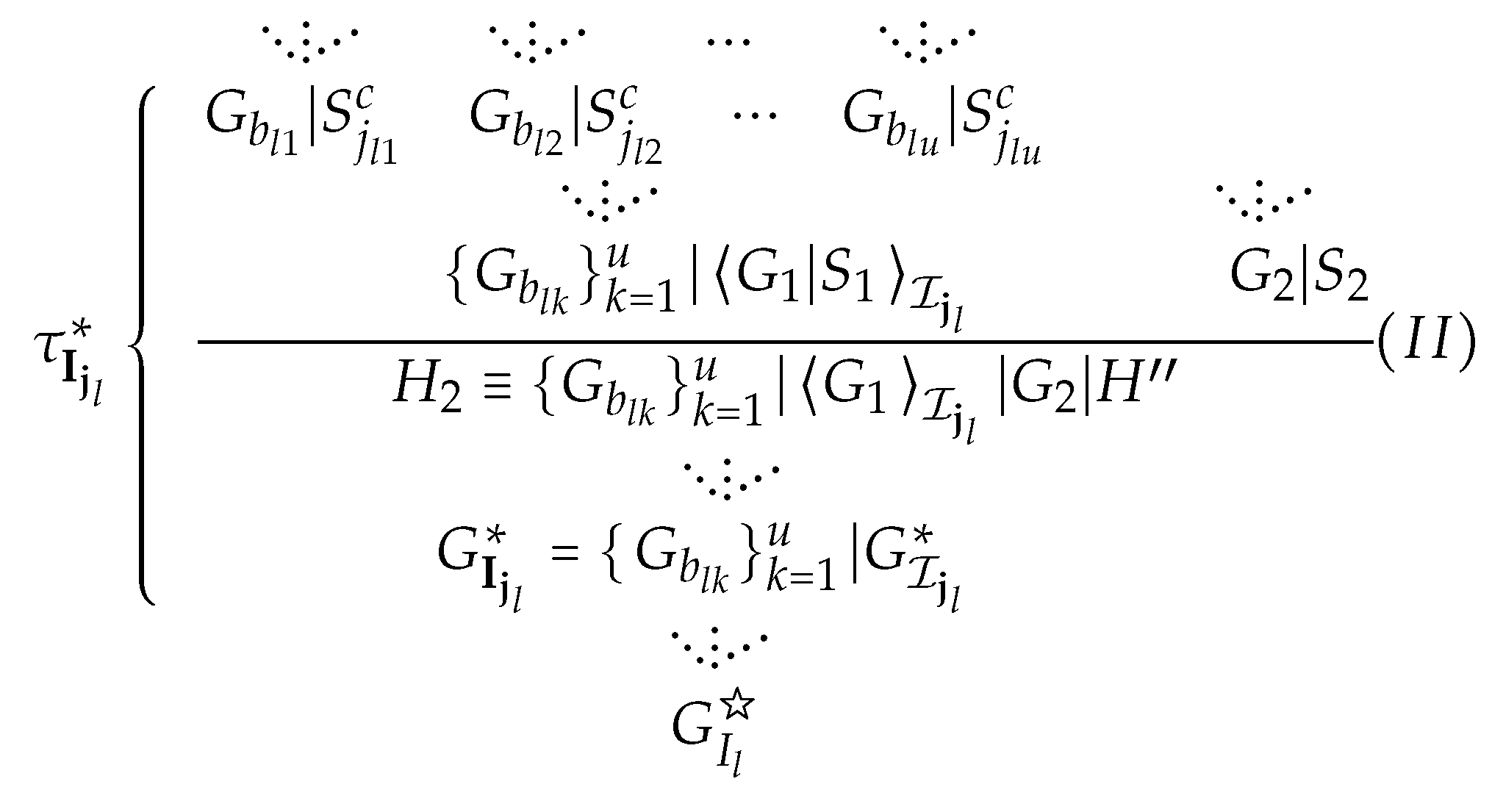
Proof. Suppose that there exist two copies ${\left\{G_{H_I^V:G^{″}}^{☆(J)}|\widehat{S^{″}}\right\}}_1$ and ${\left\{G_{H_I^V:G^{″}}^{☆(J)}|\widehat{S^{″}}\right\}}_2$ of $G_{H_I^V:G^{″}}^{☆(J)}|\widehat{S^{″}}$ in $G_{{\mathbf{I}}_l}^{☆}$, and we put them into ${\{\}}_1$ and ${\{\}}_2$ in order to distinguish them. Let ${\left[S\right]}_{G_{I_l}^{☆}}$ be a splitting unit of $G_{{\mathbf{I}}_l}^{☆}$ and S its splitting sequent. Then, $\left|v_l(S)\right|+\left|v_r(S)\right|⩾2$. Thus, S is a $(pEC)$-sequent and has the form $S_i^c$ by ${\left[S\right]}_{G_{I_l}^{☆}}{\subseteq }_{c}G|G^{*}$. Then, ${[S]}_{G_{I_l}^{☆}}={[S_i^c]}_{G_{I_l}^{☆}}$, $H_i^c\parallel H_j^c$ for all $H_j^c\in I_l$ and $S_i^c\in G_{{\mathcal{I}}_{{\mathbf{j}}_l}}^{*}$ for some ${\tau }_{{\mathbf{I}}_{{\mathbf{j}}_l}}^{*}\in {\tau }_{I_l}^{☆}$ by Claim (iv). Since $I_l$ is complete and $G^{\prime }|S^{\prime }⩽H_{I_l}^V$, then $H_i^c\parallel G^{\prime }|S^{\prime }$.

Let ${\tau }_{{\mathbf{I}}_{{\mathbf{j}}_l}}^{*}$ be in the form $\frac{\underline{G_{b_{l1}}|S_{j_{l1}}^c{G}_{b_{l2}}|S_{j_{l2}}^c\cdots G_{b_{lu}}|S_{j_{lu}}^c}}{G_{{\mathbf{I}}_{{\mathbf{j}}_l}}^{*}={\{G_{b_{lk}}\}}_{k=1}^u|G_{{\mathcal{I}}_{{\mathbf{j}}_l}}^{*}}〈{\tau }_{{\mathbf{I}}_{{\mathbf{j}}_l}}^{*}〉,\frac{G_1|S_1{G}_2|S_2}{H_1\equiv G_1|G_2|H^{″}}(II)\in {\tau }^{*},$ where $G_1|S_1⩽G^{\prime }|S^{\prime }$, $G_2|S_2⩽H_i^c$, $G_1|G_2|H^{″}$ is the intersection node of $H_i^c$ and $G^{\prime }|S^{\prime }$, as shown in Figure 3. Then, $\frac{{\{G_{b_{lk}}\}}_{k=1}^u|{〈G_1|S_1〉}_{{\mathcal{I}}_{{\mathbf{j}}_l}}{G}_2|S_2}{H_2\equiv {\{G_{b_{lk}}\}}_{k=1}^u|{〈G_1〉}_{{\mathcal{I}}_{{\mathbf{j}}_l}}|G_2|H^{″}}(II)\in {\tau }_{{\mathbf{I}}_{{\mathbf{j}}_l}}^{*}$ by $G_1|S_1⩽G^{\prime }|S^{\prime }⩽H_{I_l}^V$ and $S_i^c\in G_{{\mathcal{I}}_{{\mathbf{j}}_l}}^{*}$. Since $S_2$ is separable in $G_{I_l}^{☆}$ by $G^{\prime }|S^{\prime }⩽H_{I_l}^V$, then $S_i^c\in G_2|S_2$ and $S_i^c$ is not $S_2$.

Before proceeding to prove Property (A), we present the following property of ${\left[S_i^c\right]}_{G_{I_l}^{☆}}$.

Property (B) The set of splitting sequents of ${\left[S_i^c\right]}_{G_{I_l}^{☆}}$ is equal to that of ${\left[S_i^c\right]}_{G_2|S_2}$.

Proof. 

Let $\frac{G_1^{\prime }|S_1^{\prime }{G}_2^{\prime }|S_2^{\prime }}{H_1^{\prime }\equiv G_1^{\prime }|G_2^{\prime }|H^{‴}}(II)\in {\tau }^{*}$, $G_1^{\prime }|S_1^{\prime }⩽H_1$ and $S_1^{\prime }\in {〈G_1^{\prime }|S_1^{\prime }〉}_{{\mathcal{I}}_{{\mathbf{j}}_l}}$. Then, $S_1^{\prime }$ and $S_2^{\prime }$ are separable in $G_{I_l}^{☆}$. Thus, $G_{H_1^{\prime }:G_2^{\prime }}^{☆(J)}|\widehat{S_2^{\prime }}\subseteq G_{I_l}^{☆}$ is closed. Hence, $G_{H_1:G_2}^{☆(J)}|\widehat{S_2}-{\bigcup }_{G_2^{\prime }|S_2^{\prime }}{G}_{H_1^{\prime }:G_2^{\prime }}^{☆(J)}|\widehat{S_2^{\prime }}$ is closed, where $G_2^{\prime }|S_2^{\prime }$ in ${\bigcup }_{G_2^{\prime }|S_2^{\prime }}$ runs over all $II\in {\tau }^{*}$ above such that $G_{H_1^{\prime }:G_2^{\prime }}^{☆(J)}|\widehat{S_2^{\prime }}\subseteq G_{H_1:G_2}^{☆(J)}|\widehat{S_2}$. Therefore, $v(G_{H_1:G_2}^{☆(J)}|\widehat{S_2}-{\bigcup }_{G_2^{\prime }|S_2^{\prime }}{G}_{H_1^{\prime }:G_2^{\prime }}^{☆(J)}|\widehat{S_2^{\prime }})=v(G_2|S_2)$, $\{S_j^c:S_j^c\in G_2|S_2,H_j^c⩾G_2|S_2\}=\{S_j^c:S_j^c\in G_{H_1:G_2}^{☆(J)}|\widehat{S_2}-{\bigcup }_{G_2^{\prime }|S_2^{\prime }}{G}_{H_1^{\prime }:G_2^{\prime }}^{(J)}|\widehat{S_2^{\prime }}\}$ and ${\left[S_i^c\right]}_{G_{I_l}^{☆}}\subseteq G_{H_1:G_2}^{☆(J)}|\widehat{S_2}-{\bigcup }_{G_2^{\prime }|S_2^{\prime }}{G}_{H_1^{\prime }:G_2^{\prime }}^{☆(J)}|\widehat{S_2^{\prime }}$. Then, the set of splitting sequents of ${\left[S_i^c\right]}_{G_{I_l}^{☆}}$ is equal to that of ${\left[S_i^c\right]}_{G_2|S_2}$ since each splitting sequent $S^{‴}\in {\left[S_i^c\right]}_{G_{I_l}^{☆}}$ is a $(pEC)$-sequent by $\left|v_l(S^{‴})\right|+\left|v_r(S^{‴})\right|⩾2$ and $S^{‴}{\in }_{c}G|G^{*}$. This completes the proof of Property (B). □

We therefore assume that, without loss of generality, $S_i^c$ is in the form $\Gamma ,p_k,\Delta \Rightarrow p_k$ by Property (B), Lemma 5 and the observation that each derivation-splicing operation is local. There are two cases to be considered in the following.

Case 1. 

$S_1\notin {〈G_1|S_1〉}_{G_b|S_j^c}$ for all ${\tau }_{G_b|S_j^c}^{*}\in {\tau }_{H_I^V:G^{″}}^{☆(J)}$, $G_1|S_1⩽H_j^c⩽H_I^V$. Then, $G_{H_1:G_2}^{☆(J)}\bigcap G_{H_I^V:G^{″}}^{☆(J)}=\varnothing$. We assume that, without loss of generality, ${〈G_2|S_2〉}_k^{-}=G_2^{\prime }|\Gamma \Rightarrow t$, ${〈G_2|S_2〉}_k^{+}=G_2^{″}|S_2|\Delta \Rightarrow t$. Then, ${〈G_{I_l}^{☆}〉}_k^{-}=G_{H_2:G_2^{\prime }}^{☆(J)}|\Gamma \Rightarrow t$ since $S=\Gamma ,p_k,\Delta \Rightarrow p_k$ isn’t a focus sequent at all nodes from $G_2|S_2$ to $G_{I_l}^{☆}$ in ${\tau }_{I_l}^{☆}$ and, $H_j^c⩽H_1$ or $H_j^c||G_1|S_1$ for all $S_j^c\in G_2^{\prime }$ by Lemma 6.7 in [10]. Thus, ${〈G_{I_l}^{☆}〉}_k^{-}\setminus \Gamma \Rightarrow t\subseteq G_{H_2:G_2}^{☆(J)}$. Therefore, ${\left\{G_{H_I^V:G^{″}}^{☆(J)}|\widehat{S^{″}}\right\}}_1|{\left\{G_{H_I^V:G^{″}}^{☆(J)}|\widehat{S^{″}}\right\}}_2\subseteq {〈G_{I_l}^{☆}〉}_k^{+}$ because ${\left[S\right]}_{G_{I_l}^{☆}}\subseteq G_{H_2:G_2}^{☆(J)}|\widehat{S_2}$, $G_{H_2:G_2}^{☆(J)}|\widehat{S_2}\bigcap ({\left\{G_{H_I^V:G^{″}}^{☆(J)}|\widehat{S^{″}}\right\}}_1|{\left\{G_{H_I^V:G^{″}}^{☆(J)}|\widehat{S^{″}}\right\}}_2)=\varnothing$ and ${〈G_{I_l}^{☆}〉}_k^{-}\setminus \{\Gamma \Rightarrow t\}|{〈G_{I_l}^{☆}〉}_k^{+}\setminus \{\Delta \Rightarrow t\}|\Gamma ,p_k,\Delta \Rightarrow p_k=G_{I_l}^{☆}$. This shows that any splitting unit ${\left[S\right]}_{G_{I_l}^{☆}}$ outside $G_{H_I^V:G^{″}}^{☆(J)}|\widehat{S^{″}}$ in $G_{{\mathbf{I}}_l}^{☆}$ doesn’t take two copies of $G_{H_I^V:G^{″}}^{☆(J)}|\widehat{S^{″}}$ apart, i.e., the case of ${\left\{G_{H_I^V:G^{″}}^{☆(J)}|\widehat{S^{″}}\right\}}_1\subseteq {〈G_{I_l}^{☆}〉}_k^{-}$ and ${\left\{G_{H_I^V:G^{″}}^{☆(J)}|\widehat{S^{″}}\right\}}_2\subseteq {〈G_{I_l}^{☆}〉}_k^{+}$ doesn’t happen.

Case 2. 

$S_1\in {〈G_1|S_1〉}_{G_b|S_j^c}$ for some ${\tau }_{G_b|S_j^c}^{*}\in {\tau }_{H_I^V:G^{″}}^{☆(J)}$, $G_1|S_1⩽H_j^c⩽H_I^V$. Then, $G_b|{〈G_1〉}_{S_j^c}|G_2|H^{″}\in {\tau }_{G_b|S_j^c}^{*}$. Thus, $G_{H_1:G_2}^{☆(J)}|\widehat{S_2}\subseteq G_{H_I^V:G^{″}}^{☆(J)}|\widehat{S^{″}}$. Hence, ${\left[S_i^c\right]}_{G_{I_l}^{☆}}\subseteq G_{H_I^V:G^{″}}^{☆(J)}|\widehat{S^{″}}$. The case of $S_i^c\in G^{″}$ is tackled with the same procedure as the following. Let ${\left[S_i^c\right]}_{G_{I_l}^{☆}}\subseteq {\left\{G_{H_I^V:G^{″}}^{☆(J)}|\widehat{S^{″}}\right\}}_1$. Then, there exists a copy of ${\left[S\right]}_{G_{I_l}^{☆}}$ in ${\left\{G_{H_I^V:G^{″}}^{☆(J)}|\widehat{S^{″}}\right\}}_2$ and let $\Gamma ,p_{k^{\prime }},\Delta \Rightarrow p_{k^{\prime }}$ be its splitting sequent. We put two splitting units into ${\{\}}_k$ and ${\{\}}_{k^{\prime }}$ in order to distinguish them. Then, ${\{{\left[S\right]}_{G_{I_l}^{☆}}\}}_k\subseteq {\left\{G_{H_I^V:G^{″}}^{☆(J)}|\widehat{S^{″}}\right\}}_1$ and ${\{{\left[S\right]}_{G_{I_l}^{☆}}\}}_{k^{\prime }}\subseteq {\left\{G_{H_I^V:G^{″}}^{☆(J)}|\widehat{S^{″}}\right\}}_2$. We assume that, without loss of generality, ${〈G_2|S_2〉}_k^{-}=G_2^{\prime }|\Gamma \Rightarrow t$, ${〈G_2|S_2〉}_k^{+}=G_2^{″}|S_2|\Delta \Rightarrow t$. Then, ${〈G_{I_l}^{☆}〉}_k^{-}\setminus \{\Gamma \Rightarrow t\}\subseteq {\left\{G_{H_I^V:G^{″}}^{☆(J)}|\widehat{S^{″}}\right\}}_1$. Thus, ${\{{\left[S\right]}_{G_{I_l}^{☆}}\}}_{k^{\prime }}\subseteq {\left\{G_{H_I^V:G^{″}}^{☆(J)}|\widehat{S^{″}}\right\}}_2\subseteq {〈G_{I_l}^{☆}〉}_k^{+}$ by ${〈G_{I_l}^{☆}〉}_k^{-}\setminus \{\Gamma \Rightarrow t\}\bigcup {〈G_{I_l}^{☆}〉}_k^{+}\setminus \{\Delta \Rightarrow t\}=G_{I_l}^{☆}\setminus \Gamma ,p_k,\Delta \Rightarrow p_k$. Then, ${〈{〈G_{I_l}^{☆}〉}_k^{+}〉}_{k^{\prime }}^{-}={〈G_{I_l}^{☆}〉}_{k^{\prime }}^{-}$, ${\{\Delta \Rightarrow t\}}_k{|\{\Delta \Rightarrow t\}}_{k^{\prime }}\subseteq {〈{〈G_{I_l}^{☆}〉}_k^{+}〉}_{k^{\prime }}^{+}$, where we put two copies of $\Delta \Rightarrow t$ into ${\{\}}_k$ and ${\{\}}_{k^{\prime }}$ in order to distinguish them. Then, $\Gamma \Rightarrow t\in {〈G_{I_l}^{☆}〉}_{k^{\prime }}^{-}$, ${⊢}_{\mathbf{GL}}{〈G_{I_l}^{☆}〉}_k^{-}$, ${⊢}_{\mathbf{GL}}{〈G_{I_l}^{☆}〉}_{k^{\prime }}^{-}$ and ${〈G_{I_l}^{☆}〉}_{k^{\prime }}^{-}$ is a copy of ${〈G_{I_l}^{☆}〉}_k^{-}$. Then, $\mathcal{D}({〈G_{I_l}^{☆}〉}_k^{-})=\mathcal{D}({〈G_{I_l}^{☆}〉}_{k^{\prime }}^{-})\subseteq \mathcal{D}(G_{I_l}^{☆})$ could be cut off of one of them because they are the two same sets of hypersequents in $\mathcal{D}(G_{I_l}^{☆})$. Meanwhile, two copies of $\Delta \Rightarrow t$ in ${〈{〈G_{I_l}^{☆}〉}_k^{+}〉}_{k^{\prime }}^{+}$ can’t be taken apart by any splitting unit outside $G_{H_I^V:G^{″}}^{☆(J)}|\widehat{S^{″}}$ in $G_{I_l}^{☆}$ for the reason as shown in Case 1 and thus could be contracted into one by $(EC)$ in $\mathcal{D}(G_{I_l}^{☆})$. Therefore, two copies ${\left\{G_{H_I^V:G^{″}}^{☆(J)}|\widehat{S^{″}}\right\}}_1$ and ${\left\{G_{H_I^V:G^{″}}^{☆(J)}|\widehat{S^{″}}\right\}}_2$ of $G_{H_I^V:G^{″}}^{☆(J)}|\widehat{S^{″}}$ can be contracted into one in $G_{I_l}^{☆}$ by $〈E{C}_{\Omega }^{*}〉$. This completes the proof of Property (A). □

With Property (A), all manipulations in the old main algorithm in [10] work well. This completes the construction of ${\tau }_I^{☆}$ and the proof of Theorem 4. □

Theorem 5.

The standard completeness holds for ${\mathbf{HpsUL}}^{*}$.

Proof. 

Let $\underset{}{\stackrel{i}{⟷}}$ denote the i-th logical link of iff in the following. ${\vDash }_{\mathcal{K}}A$ means that $v(A)⩾t$ for every algebra $\mathcal{A}$ in $\mathcal{K}$ and valuation v on $\mathcal{A}$. Let ${\mathbf{psUL}}^{*}$, $\mathrm{LIN}({\mathbf{psUL}}^{*})$, ${\mathbf{psUL}}^{*D}$ and ${[0,1]}_{{\mathbf{psUL}}^{*}}$ denote the classes of all ${\mathbf{psUL}}^{*}$-algebras, ${\mathbf{psUL}}^{*}$-chain, dense ${\mathbf{psUL}}^{*}$-chain and standard ${\mathbf{psUL}}^{*}$-algebras (i.e., their lattice reducts are $[0,1]$), respectively. 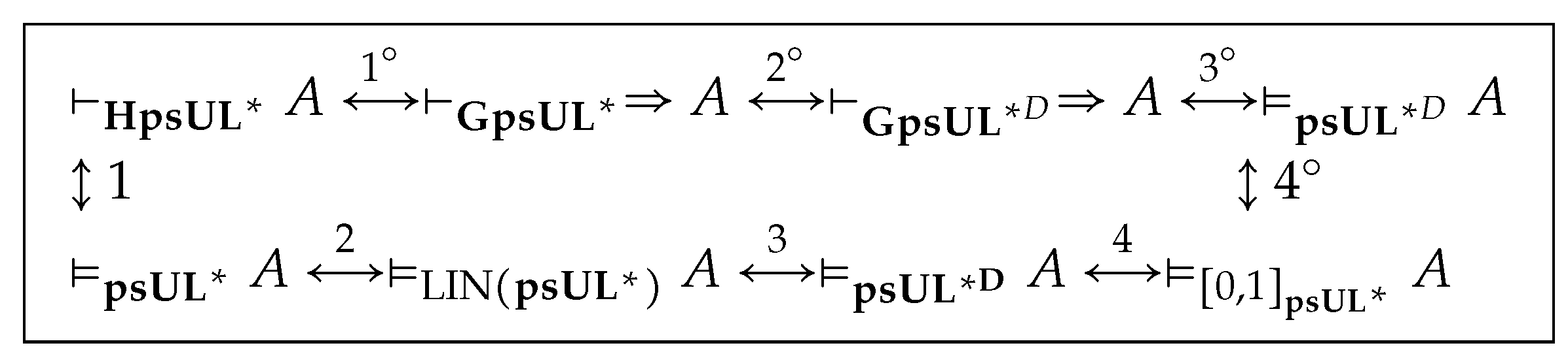We have an inference sequence, as shown in Figure 4.

Links from 1 to 4 show Jenei and Montagna’s algebraic method to prove standard completeness and, currently, it seems hopeless to build up link 3 (see [11,12,13,14]). Links from $1^{\circ }$ to $4^{\circ }$ show Metcalfe and Montagna’s proof-theoretical method. Density elimination is at Link $2^{\circ }$ in Figure 4 and other links are proved by standard procedures with minor revisions and omitted (see [1,4,15,16,17]). □

5. Future Works

Generally, for any existing fuzzy logic system, we can consider its corresponding non-commutative system, just as $\mathbf{HpsUL}$ is obtained by removing the commutativity of the strong conjunctive connective ⊙ in $\mathbf{UL}$. Therefore, we can consider the corresponding non-commutative systems of many systems. A natural question is whether the method of the density elimination proposed in this paper can be generalized to these systems. It has often been the case in the past that metamathematical methods have corresponding algebraic analogues. The method proposed in this paper is essentially proof-theoretic. A natural problem is whether there is an algebraic proof corresponding to our proof-theoretic one.