Coupling Conditions for Water Waves at Forks


1
Laboratoire de Mathématiques, INSA Rouen Normandie, 76801 Saint–Etienne du Rouvray, France
2
University Grenoble Alpes, University Savoie Mont Blanc, CNRS, LAMA, 73000 Chambéry, France
*
Author to whom correspondence should be addressed.
Symmetry 2019, 11(3), 434; https://doi.org/10.3390/sym11030434
Submission received: 15 January 2019
/
Revised: 15 March 2019
/
Accepted: 19 March 2019
/
Published: 24 March 2019
(This article belongs to the Special Issue Symmetries of Nonlinear PDEs on Metric Graphs and Branched Networks)
Abstract
:We considered the propagation of nonlinear shallow water waves in a narrow channel presenting a fork. We aimed at computing the coupling conditions for a 1D effective model, using 2D simulations and an analysis based on the conservation laws. For small amplitudes, this analysis justifies the well-known Stoker interface conditions, so that the coupling does not depend on the angle of the fork. We also find this in the numerical solution. Large amplitude solutions in a symmetric fork also tend to follow Stoker’s relations, due to the symmetry constraint. For non symmetric forks, 2D effects dominate so that it is necessary to understand the flow inside the fork. However, even then, conservation laws give some insight in the dynamics.
1. Introduction
The propagation of nonlinear waves in a network is an important topic. As an example, consider a hydrological network which is prone to floods. Understanding the global dynamics of the network can help identify its most vulnerable sections and take the appropriate measures. Real networks are formed by long 2D or 3D channels of a small cross-section. To study the propagation of waves in such systems, a first step is to consider a simple fork as a model of elementary junctions. The final goal is to reduce the model to 1D channels connected by appropriate interface conditions. The study of such 1D systems is now well advanced, in particular for systems of conservation laws, see the review [1].
The type of PDE model describing the quantity propagating on the network is very important to derive the coupling conditions. Recently for the sine-Gordon nonlinear wave equation, we [2] introduced a homothetic reduction [3] where we averaged the operator over the fork region and consistently took the limit when the width tended to zero. Assuming continuity of the field, we obtained Kirchhoff’s law for the gradients. Comparing the 2D solution with the one for the reduced 1D equations gives excellent agreement. In this situation, the angle of the fork does not play a role. When considering networks of rivers, many authors, for example Stoker [4] and Jacovkis [5] assumed continuity of the water height and continuity of the flux so that again, the angle of the fork did not come in. In the close context of gas dynamics, Holden and Risebro [6] studied shocks in a pipe with an elbow. They showed that the Riemann problem had a unique solution when the angle was smaller than . The angle is also important for classical hydrodynamics; in a fork, it sets the forces experienced by the pipes [7]. In fact, for large amplitude shallow water waves our numerical calculations show that the energy entering a branch can vary from 20% to 50% depending on the symmetry of the fork. These studies point out the importance of the angle.
A few authors addressed the problem of the angle of a junction. Schmidt [8] studied the 2D connection between 1D channels; he made no assumption on the size of the connecting domain. The flow in the junction was assumed linear so that the author used a variational method that gave the solution as a superposition of fields. The final result was a system of ordinary differential equations for the values at the ends of the branches coupled to the shallow water PDEs. Despite its formal beauty, it remains difficult to handle and does not give a simple picture. Shi et al. [9] studied experimentally and numerically the propagation of long waves in wide and narrow channels. They used the Boussinesq dispersive shallow water equations for narrow channels. They observed no angle dependence and a strong transmission. For the same equations, Nachbin and Simoes [10] obtained interface conditions containing implicitly the angles of the fork. These gave an excellent matching between the average of the 2D solution and the solution of the 1D effective model for angles smaller than .
In this article, we consider the nonlinear shallow water equations. The system is very general because it only involves conservation laws. Also it is simple enough. We revisit the problem of shallow water propagation in 2D forks using our homothetic reduction procedure to obtain approximate conservation laws and compare them with the numerical solutions. We compute approximate conservation for the mass, momenta and energy laws for a general fork geometry. In the small amplitude limit we recover Stoker’s conditions, i.e., continuity of surface elevation and mass conservation (Kirchoff law). To our knowledge, this is a first formal justification of Stoker’s interface conditions. This angle independent reduction holds also for a general class of scalar nonlinear wave equations, for example the 2D sine-Gordon equation or the 2D reaction-diffusion equation; it confirms the results of [2]. We computed the 2D numerical solution for a simple T-fork geometry for small and large amplitudes. The wave was also launched in two different branches to see the effect of symmetry. We show that Stoker’s conditions hold for the symmetric case for small and large amplitudes. For the non-symmetric case, they hold for small amplitudes. When the amplitude is large, 2D effects dominate the fork region. Nevertheless the approximate conservation laws give an insight into the flow.
The article is organized as follows. Section 2 presents the fork geometry and shows the straightforward reduction for a general class of nonlinear wave equations. In Section 3 we recall the shallow water equations and their conserved quantities. Section 4 gives the integrals of these equations on the fork showing that the mass and energy laws do not involve the angles while the momenta laws do. Section 5 shows the 2D numerical solutions for symmetric and non symmetric configurations for small and large waves. There, we compare the numerical results with the conservation laws established in Section 4. We discuss these results and conclude in Section 6.
2. General Scalar Nonlinear Wave Equations
Before considering the nonlinear shallow water equations, we analyze the simpler case of a class of scalar 2D nonlinear wave equations. This large class includes hyperbolic wave equations like the sine-Gordon equation as well as reaction diffusion equations like the Fisher equation, to name a few. We consider equations of the form
where is a scalar, is the usual 2D Laplacian and where is a nonlinearity not containing derivatives. The boundary condition on the lateral domain is of Neumann type
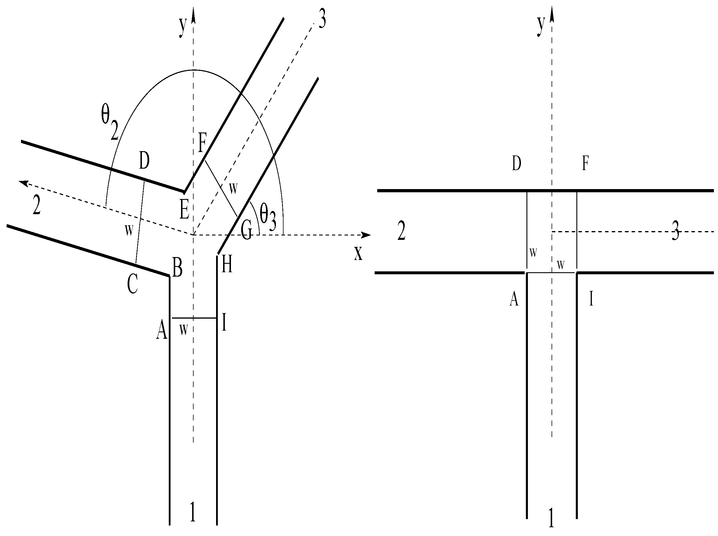
Consider the fork domain shown in Figure 1. Far from the fork region, the solution can be assumed to be 1D so that we do not loose much information by approximating the 2D dynamics with a 1D equation. Inside the fork domain, a strong coupling occurs between the branches. To see this, we proceed as in [2] and integrate the operators on the fork region. Then we examine the behavior of the different terms as w, the width of the branches, goes to zero. We assume that domains that we consider behave in a regular way as we shrink w homothetically to zero, [3].
Consider the asymmetric Y-branch shown in the left panel of Figure 1. A first assumption is the continuity of u which is obvious for the 2D operator. The other condition comes from the integration of the operator (1) on the fork domain . We get
The first integral is of order . On the exterior boundaries, so the line integral reduces to
which are . We then obtain for
where are respectively the values of the field at the end of branch 1 (IA) and at the beginning of branches 2 (FG) and 3 (CD). Relation (4) is Kirchhoff’s law [2]. When the widths of the branches are not equal, this Kirchoff relation becomes
Remark that in the result (4) the angle of the fork plays no role. The reduction leading from the flux equation to (5) is an asymptotic result that holds for . It is then natural to approximate the 2D Equation (1) by a 1D equation in each branch together with the conditions of continuity and Kirchoff (4) at the junctions.
The result we obtain can be connected to a property of the Laplace operator with Neumann boundary conditions on a so-called “fat” graph [11]. Consider a graph where each edge has a transverse size w, assume Neumann boundary conditions on the transverse edge. Then the spectrum of the Laplacian converges to the one of the 1D Laplacian as . This is true for compact and non compact graphs. See the article by Exner and Post [11] and the book by Post [12] for the details of the proof.
The validity of the reduction was confirmed numerically for the 2D sine-Gordon equation, (1) with and in [2]. There we compared the 2D solutions to the ones of the 1D sine-Gordon equation in each branch, coupled by the interface conditions. For completeness, we recall the case of a sine-Gordon kink propagating in forks with angles 45 and 90 degrees. The kink is an exact solution in 1D, it is
where the velocity is a free parameter. To compare the 2D and 1D solutions, we plot the energies in each branch
and
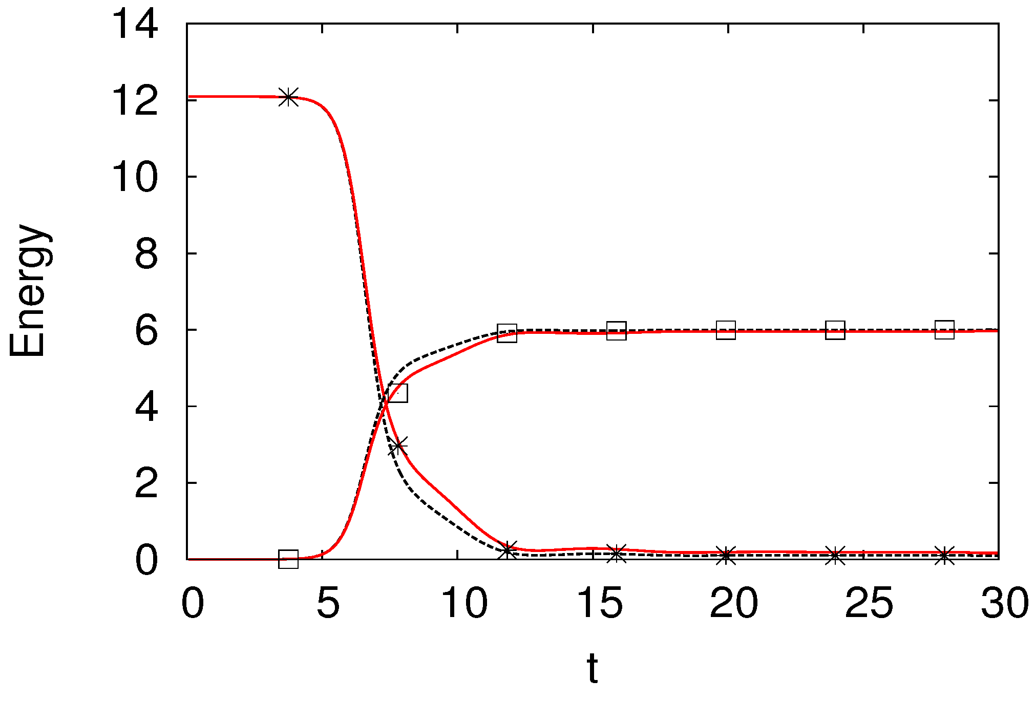
where is branch i, abusively named the same in 1D and 2D. The kink is started in branch 1 with an initial velocity , this gives a typical wavelength . The width of the branches is . Figure 2 shows the time evolution of the energies for forks with angles 45 and 90 degrees and , where corresponds to the branches. Initially the kink is in branch 1 so that . As the kink crosses into branches 2 and 3, becomes very small. Note the excellent agreement between the two expressions and the expression . This confirms that the angle of the fork plays no role for such a system.
The dynamics of kinks for the sine-Gordon equation is controlled by the energy: if the initial energy is enough, a kink in branch 1 gives rise to two kinks in branches 2 and 3. This gives a very simple picture. Other solutions like the breather have much more complicated dynamics, we refer the reader to [2] for more details.
The dynamics of such waves can then be studied for general networks as we have done in [13].
3. The Nonlinear Shallow Water Equations
The shallow water equations in a 2D domain written in terms of the fluid velocity
and the water height read [4]
where g is the gravitational acceleration. The wall boundary condition is
We assume an even bottom of the channels .
3.1. Conserved Quantities
We first recall the conserved quantities. Integrating Equations (9)–(11) over a 2D closed domain and using the boundary condition (12) we get
A localized wave will have as first conserved quantity the integral of the water elevation
The total x and y momenta
will not be conserved in the fork geometries.
A flux relation that can be deduced from the conservation laws (9)–(11) is the total energy flux
where the total energy density is
Integrating the energy flux relation over a volume we obtain that a localized wave in will have constant energy
3.2. Small Amplitude Limit
It is well known that in the linear limit, Equations (9)–(11) reduce to the linear wave equation for the water height h. To see this, consider the steady state , then the linearized system is
Taking the time derivative of the first equation and plugging in the second equation, we get the wave equation
The boundary conditions reduce to as can be seen by projecting (19) on . This equation is in the class (1).
4. Reduction of the Shallow Water Equations
The shallow water equations cannot be reduced so simply as the nonlinear scalar wave equation. In fact, it is not clear what are the right interface conditions that should be implemented for a 1D effective model. Stoker, in his well-known book [4] introduces the following interface conditions for the water elevations and branch-oriented velocities
and uses them to analyze the junction of the Mississippi and the Missouri rivers. These conditions were not justified by a formal argument. Note also that they do not depend on the angle of the junction.
Below, we will see that these conditions arise naturally in the limit of small amplitude for the shallow water equations. For general amplitudes, it is not clear that these apply. To analyze the problem, we proceed as in [2], integrate the governing equations on the bifurcation region and consider the limit of vanishing transverse width w.
4.1. Mass Flux
Integrating the Equation (9) over the closed region yields
Because of the boundary condition on ABC, DEF and GHI the expression above reduces to
The first integral is while the three other integrals are . Dividing the equation by w and taking the limit we get from these three terms
where we have introduced the local branch-oriented velocities such that
and where the indices 1,2 and 3 refer to the branches. Of course, when the transverse widths are different, with the condition that the ratios remain finite, the relation (23) becomes
4.2. Energy Flux
The energy flux (16) can be consistently reduced to a 1D relation. As for the mass relation, we integrate Equation (17) over the domain ABCDEFGHIA to obtain
Because of the boundary condition on ABE, the expression above reduces to
The first integral is while the three other integrals are . Dividing the equation by w and taking the limit we get from these three terms
To conclude, Equation (9) gives in the 1D limit, the balance of mass (23). The same happens for the energy flux (16) which yields (25). The natural matching conditions for 1D shallow water equations on a network are then
For the mass and the energy balance laws, we have a similar situation to the one of the nonlinear scalar wave equation, the angles of the fork do not play any role. In the small amplitude limit, the speeds are small and the squares can be neglected in the energy relation. Then, we recover the Stoker interface conditions (21).
4.3. Momentum Flux for a General Fork
Contrary to the mass and the energy, the momentum Equations (10) and (11) cannot be consistently reduced to a 1D condition involving at each end of .
To see this, integrate the horizontal momentum Equation (10) over the domain and get
where the first integral is a surface integral and the second one a line integral. In the integrand of the latter, we have
on the exterior boundaries of because of the boundary condition (2). Then, only the potential term will contribute to these terms.
The terms (line integrals) reduce to
Using the branch oriented velocities (24) we get the approximate law
where we neglected the velocity components .
Similarly for the vertical momentum equation we obtain
Using the branch velocities and neglecting the transverse components we get
4.4. Momentum Flux for the T-Fork
Consider now the T-geometry shown in the right panel of Figure 1. The calculations are simpler so that we used this geometry to validate the approach numerically. The general fork domain can be reduced to the square by taking and . Then the Equations (28) and (30) reduce to
where the term is
We will see that it can be obtained by interpolation of and .
4.5. Effective 1D Model for the T-Fork
The pseudo-conservation laws (26), (27), (29) and (31) established in the previous section in the limit provide a formal connection between in branches 1,2 and 3. In principle, they enable to approximate the 2D problem (9)–(11) by three 1D shallow water equations
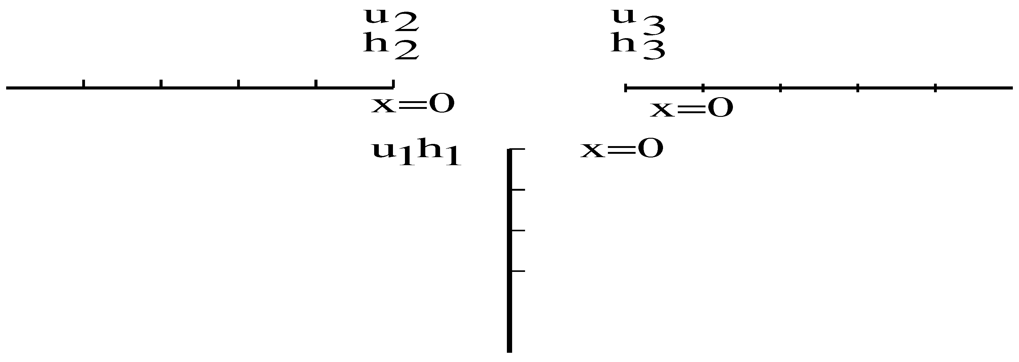
where correspond to the different branches. These 1D shallow water equations can be solved using a standard finite difference scheme, see for example [14]. The discretization is shown in Figure 3 where the first nodes in each branch have values . The coupling equations between these three nodes given by (26), (27) and (29) would be solved using a Newton iteration.
5. Numerical Solutions of the 2D Shallow Water Equations
The approximation described in the previous section holds if the error remains small. We now evaluate this error by solving numerically the 2D problem (9)–(11), compute and see how these values agree with the pseudo-conservation laws (26), (27), (29) and (31). We chose the T geometry shown in the right panel of Figure 1 for simplicity and considered symmetric and non symmetric initial conditions. We also increased the wave amplitude to estimate the effect of the non linearity.
The Equations (9)–(11) were discretized using as space unit the depth d. The time unit was . The variables and fields was rescaled as
This amounts to taking in (9)–(11).
We solved the nonlinear shallow water equations using a first order finite volume scheme on an unstructured triangular mesh produced with the Gmsh meshing software (see details in [15]). We used the width and the typical size of the triangles is . The time advance used a variable order Adams–Bashforth–Moulton multistep solver (implemented in Matlab under ode113 subroutine [16]). The relative and absolute tolerances were set to .
The initial condition is taken as a travelling solitary wave of velocity c. This is an exact solution for the mass conservation law. We used a solitary wave inspired by the Serre theory [17], (see [18] for the modern variational derivation)
where the speed is
The other parameters were
The wave was chosen so that its extension is much larger than the width . Below we discuss the effect of the width.
The four pseudo-conservation laws for the mass, momenta and energy (26), (27) and (29) on the fork domain are
where we introduced the residuals and .
We considered a symmetric situation where the wave is incident from branch 1 and a non symmetric situation where the wave was send into the fork from branch 3. In both cases, the number of unknowns was the same; see Table 1.
The wave mass and wave energy in each branch have been calculated. They are defined as
Energy will propagate very differently in problems 1 and 2. In the next sections we examine in detail the two types of problems and use the conservation laws to establish jump conditions for the 1D effective model.
To verify the approximation given by the relations (41)–(44), we also computed the time evolution of the quantities from the 2D direct numerical simulations. We used a scattered linear interpolation to estimate these physical variables along the four different segments of the fork region from the unstructured triangular mesh data.
5.1. Wave Incident into Branch 1
5.1.1. Small Amplitude Waves
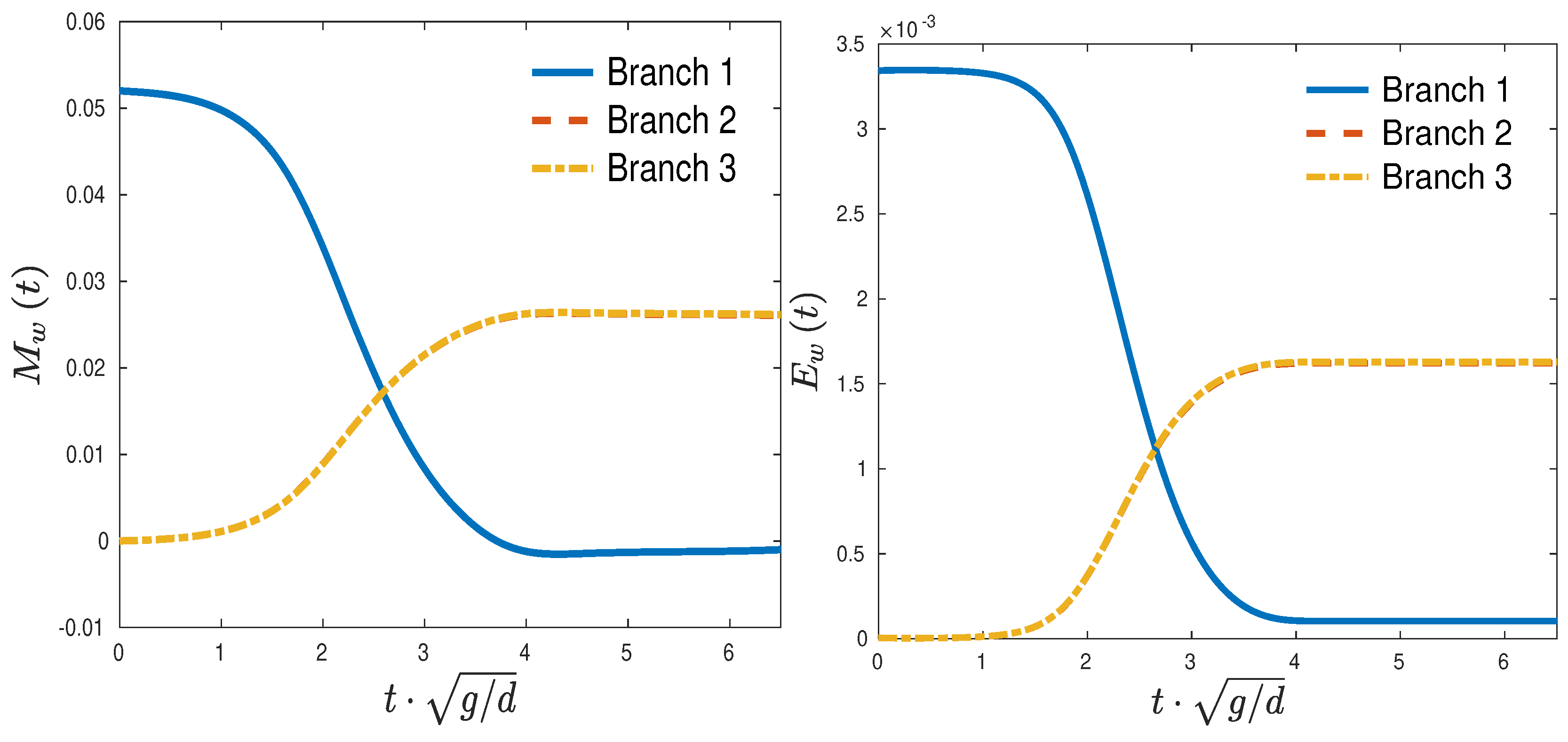
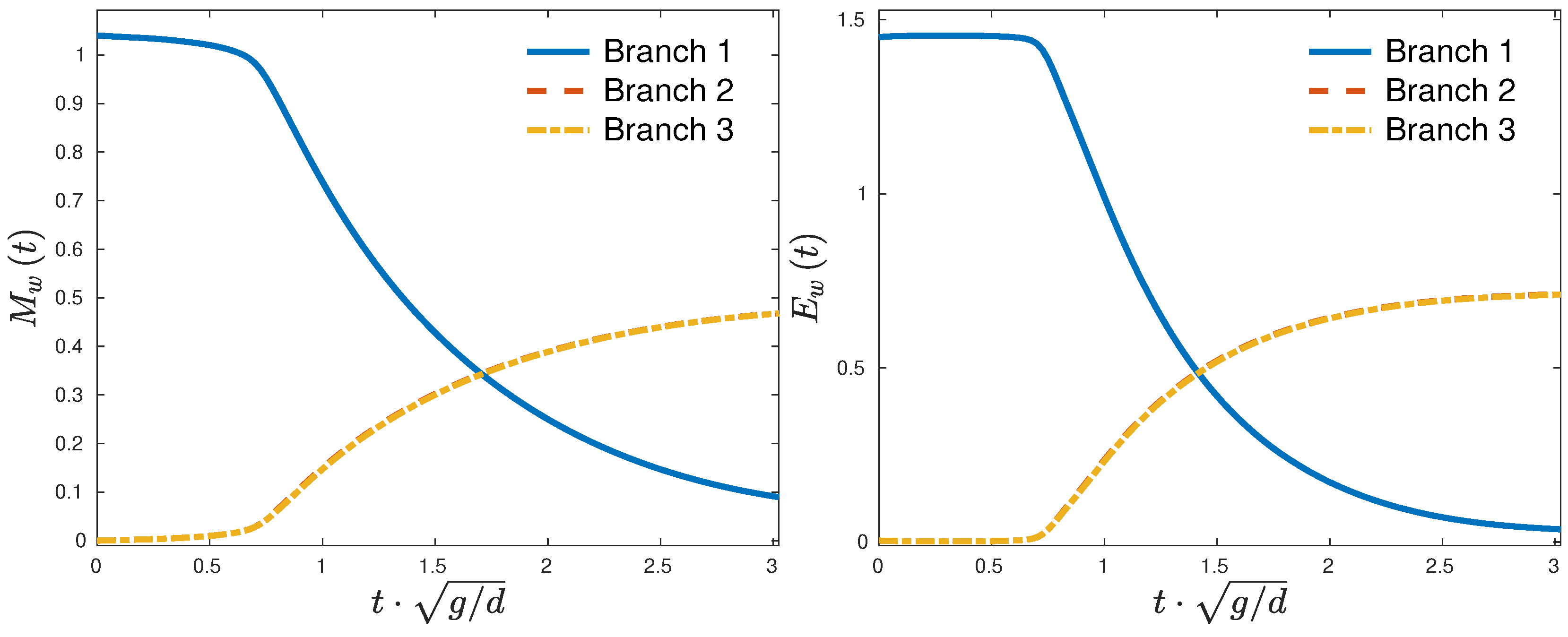
The time evolution of the wave mass and energy is presented in Figure 4. Consider the wave mass, at : . After the wave has passed, at . We have which shows the conservation of mass. Notice the depression in the mass in branch 1 after the wave passes. Almost all energy is transferred to branches 2 and 3.
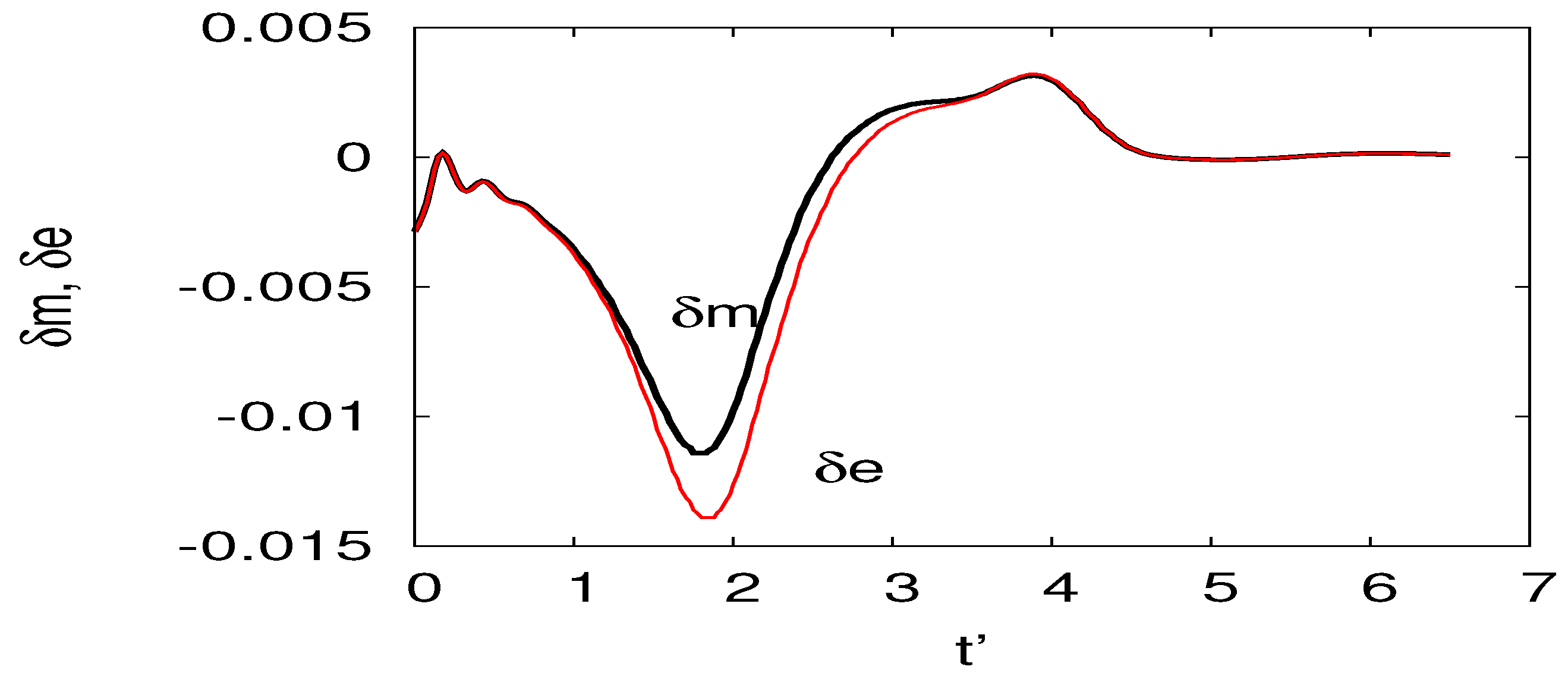
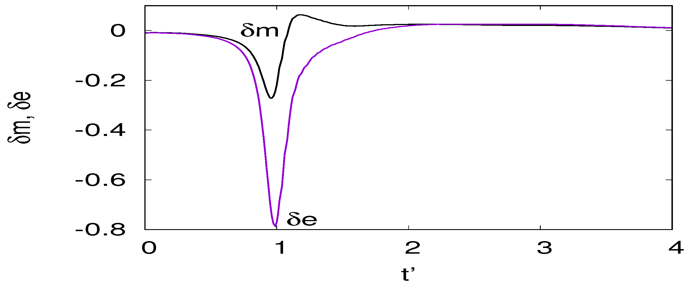
Here our balance laws hold well for both the mass and the energy, see Figure 5.
We can use them to obtain . Assume symmetry . The balance laws reduce to
Since we can neglect the terms of the second equation. The resulting relations are satisfied by
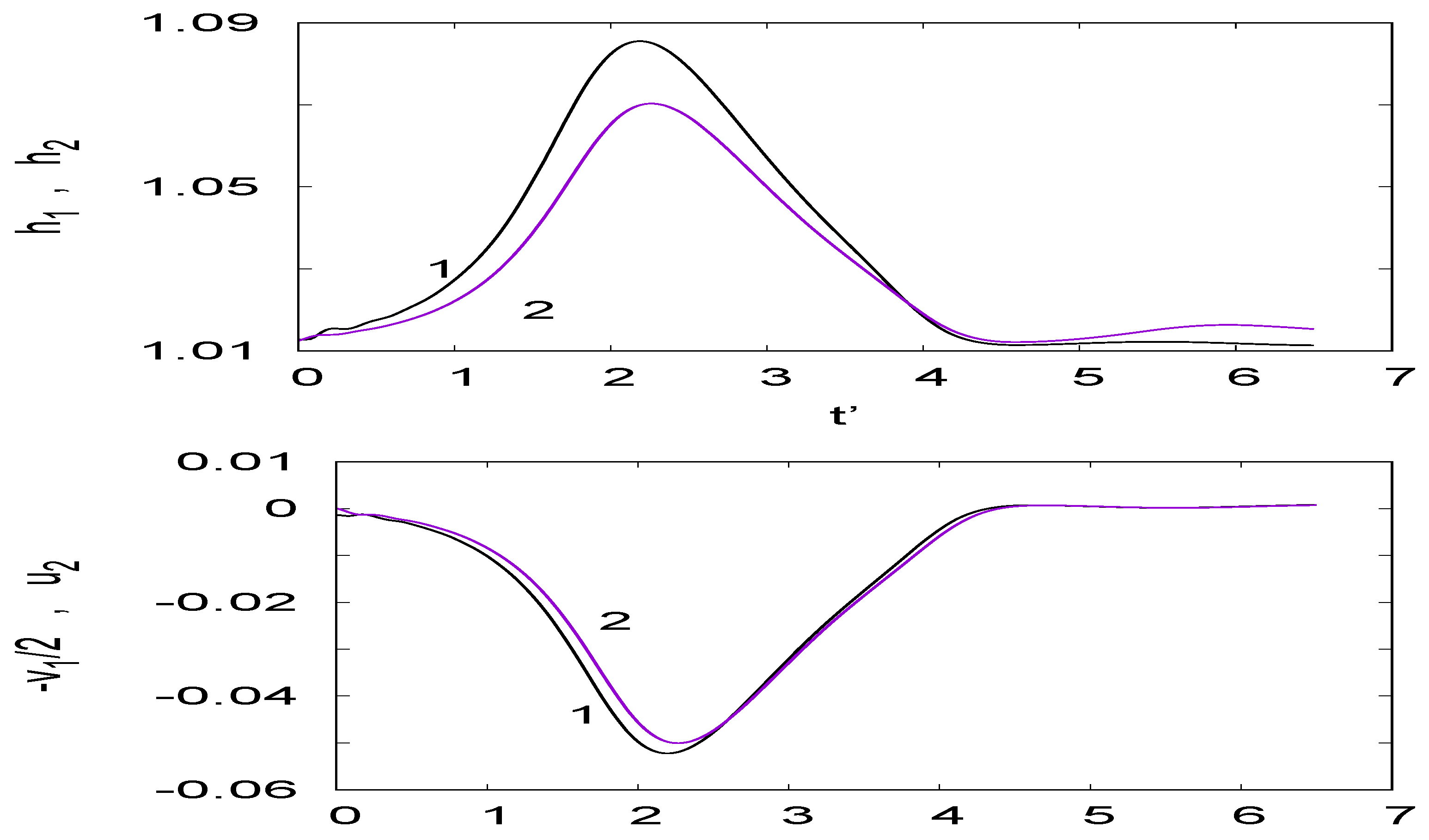
which are the Stoker conditions. These are in good agreement with the simulations as shown by Figure 6.
5.1.2. Very Large Amplitude Waves
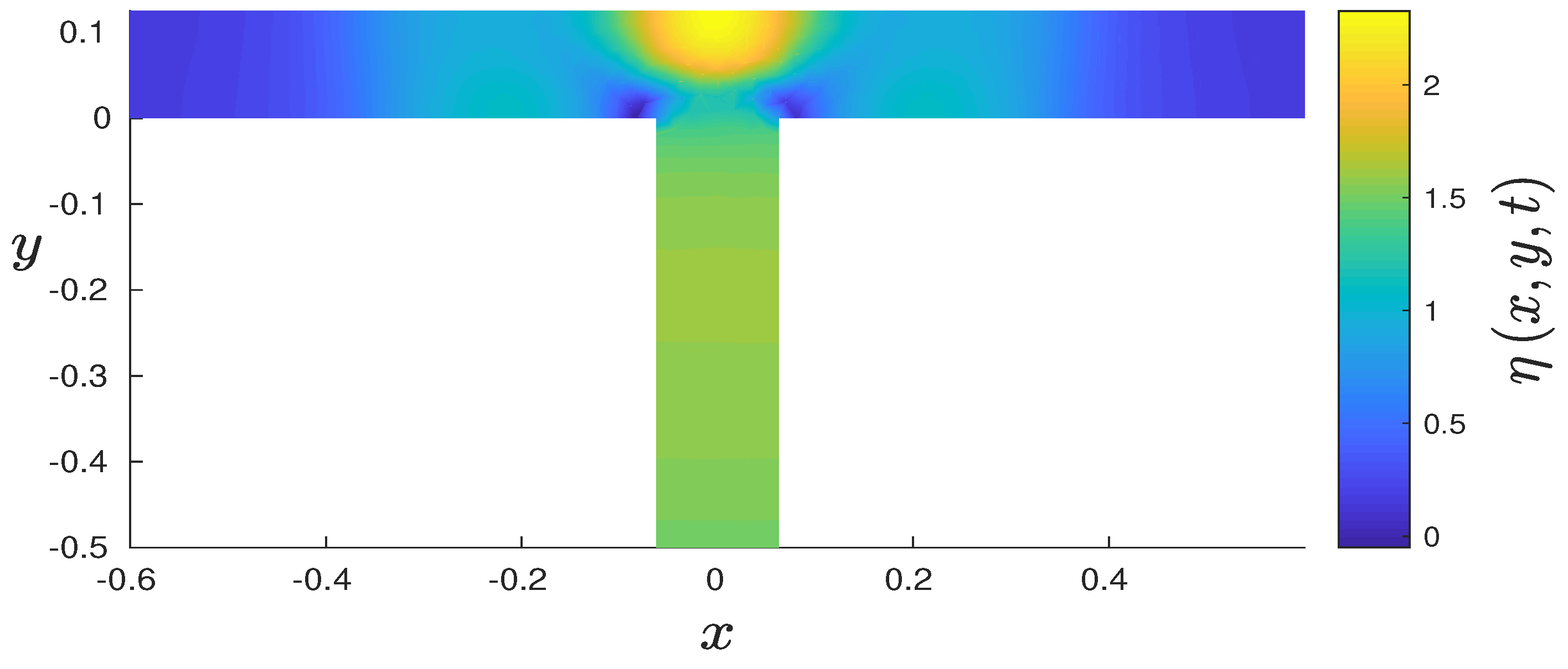
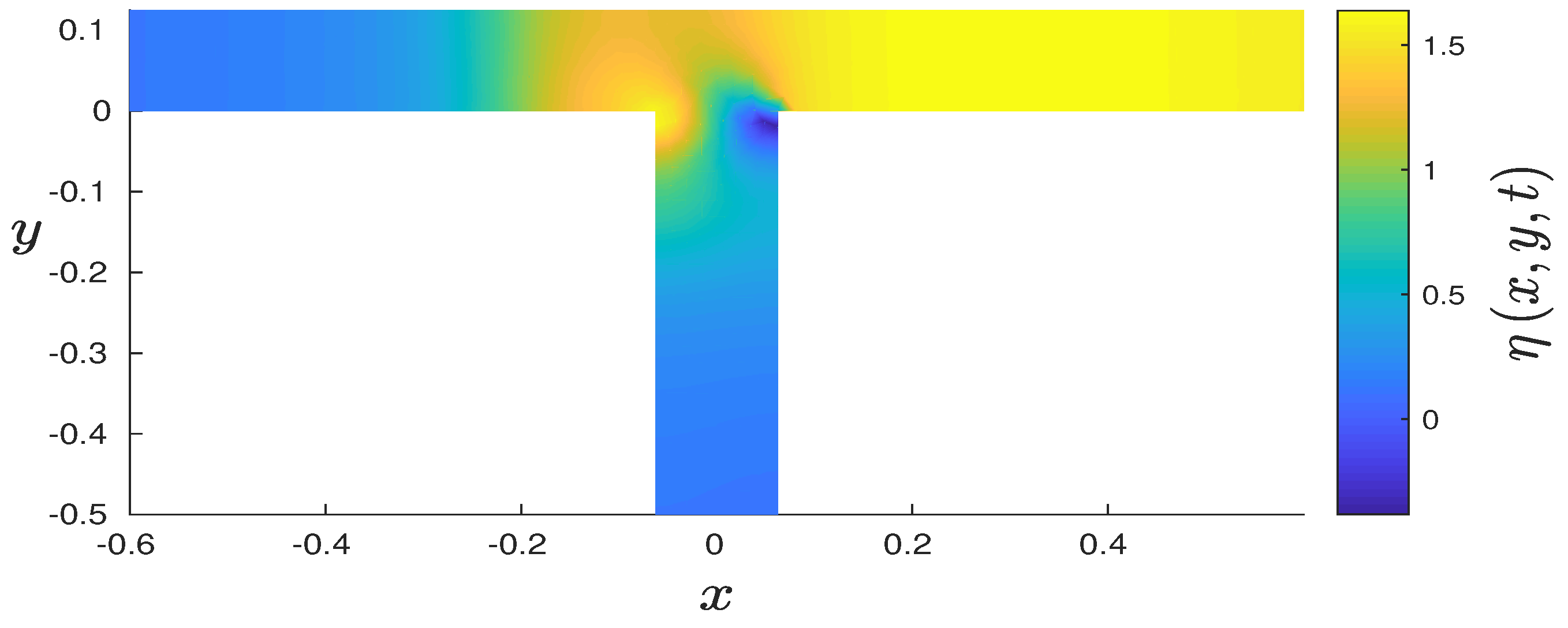
In this case, 2D effects start to appear. Figure 7 shows a snapshot of the surface elevation h for a wave such that . Notice the lump on the edge of the domain.
Figure 8 shows the time evolution of the wave mass and energy. Despite the evidence of 2D effects, the overall transfer of wave mass and wave energy from branch 1 to branches 2 and 3 does not vary significantly as changes from to 2.
Figure 9 shows the time evolution of and . Notice that the mass relation is better satisfied than the energy relation.
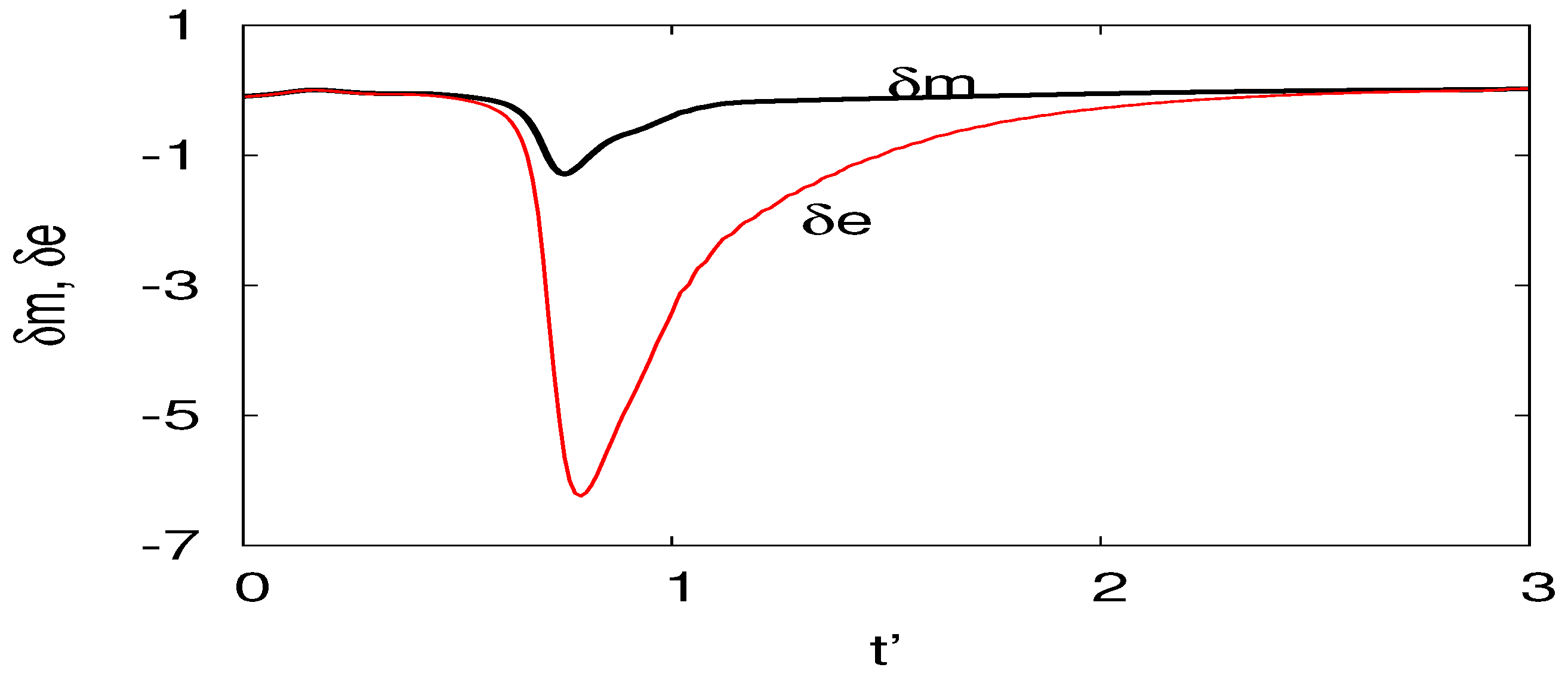
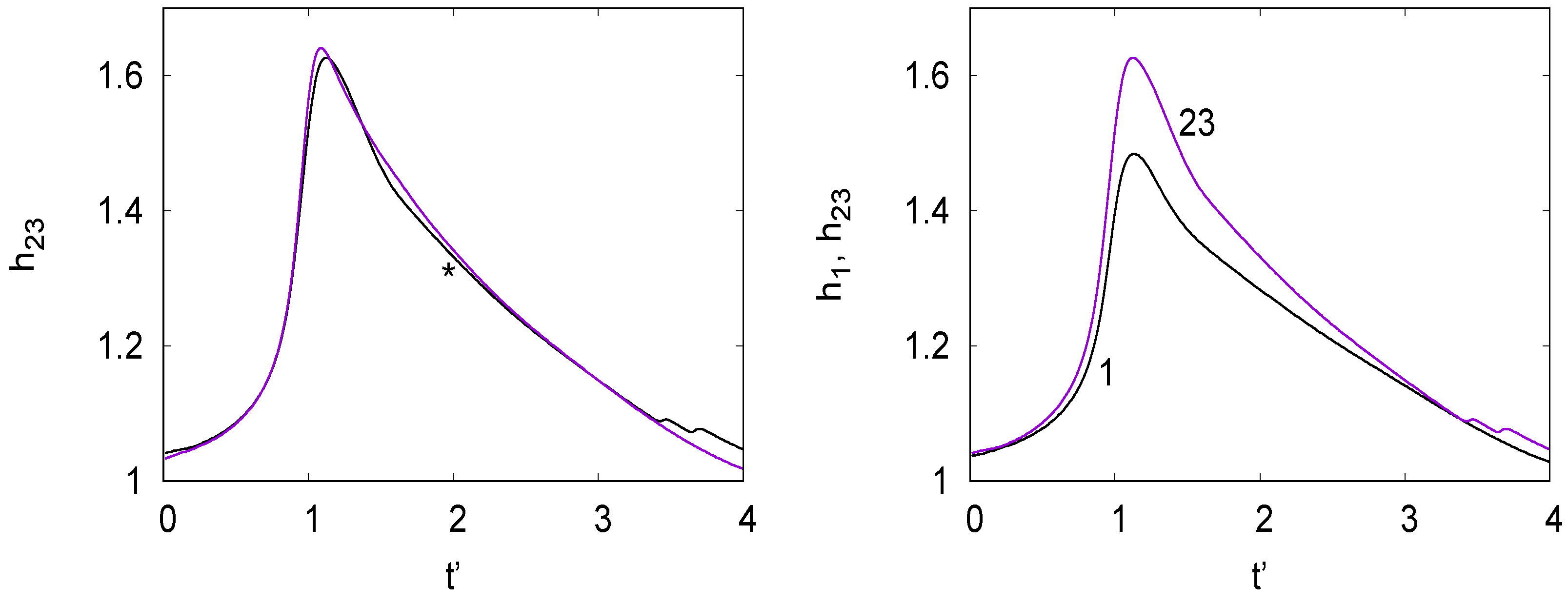
Again the Stoker relations (47) give a good approximation as shown by Figure 10 which show that and . The price to pay to approximate the 2D situation by a 1D effective model is an energy loss at the junction.
Also remark that for the approximation to hold it is crucial that the wave be wider than w and not too fast. If these conditions are not met, and will be delayed from and will need to describe what happens in the fork. We observed this for a larger channel and the same parameters.
5.2. Wave Incident into Branch 3
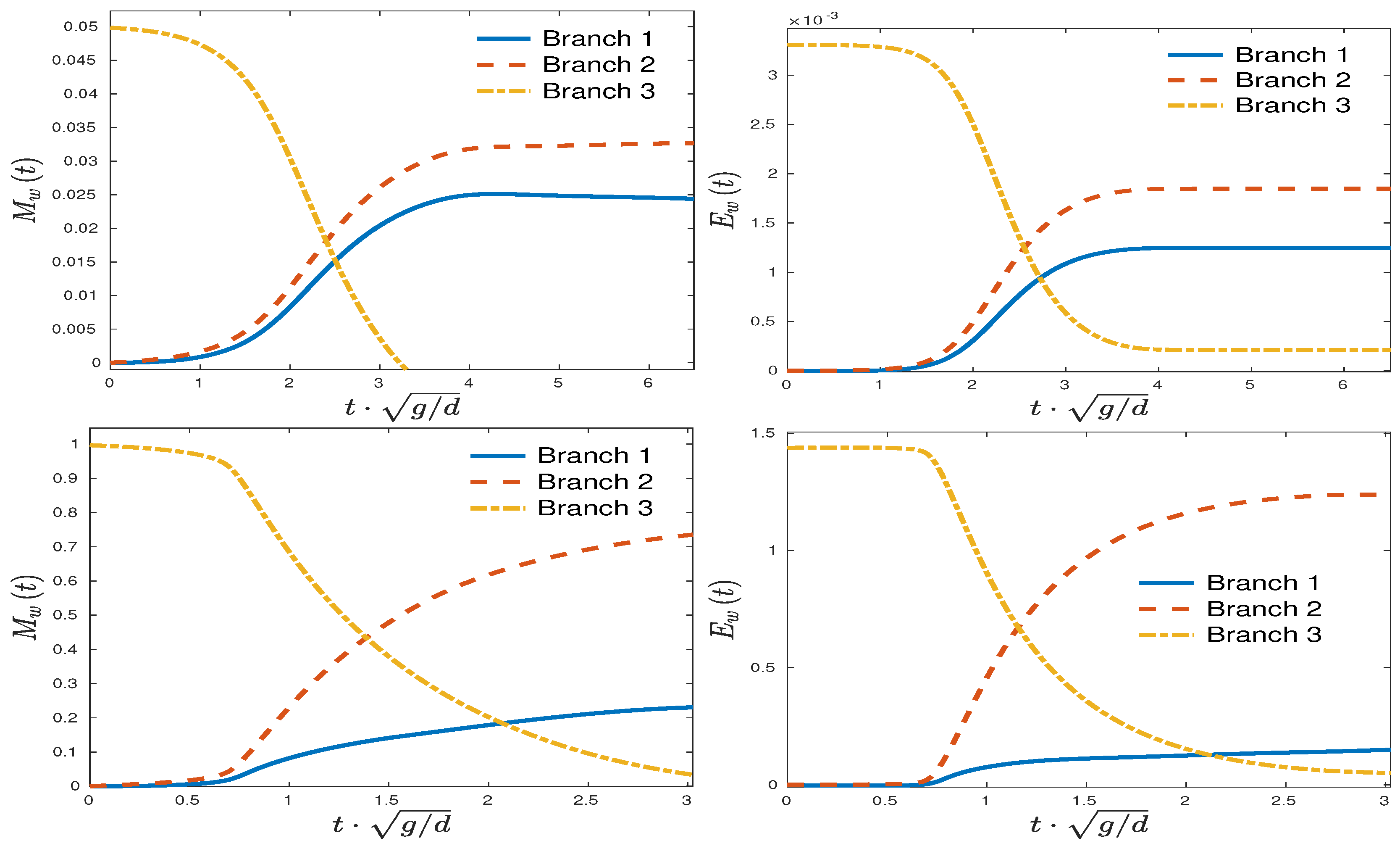
For this configuration, we observe a significant difference in behavior as the wave amplitude increases. Figure 11 shows the time evolution of the wave mass and wave energy for (top panels) and (bottom panels). Small amplitude waves get transmitted to branch 1 as much as to branch 2. On the other hand, large amplitude waves are predominantly transmitted to branch 2. The mass entering branch 2 is three times larger than the one entering branch 1; for energies, the factor is six.
5.2.1. Small Amplitude Waves
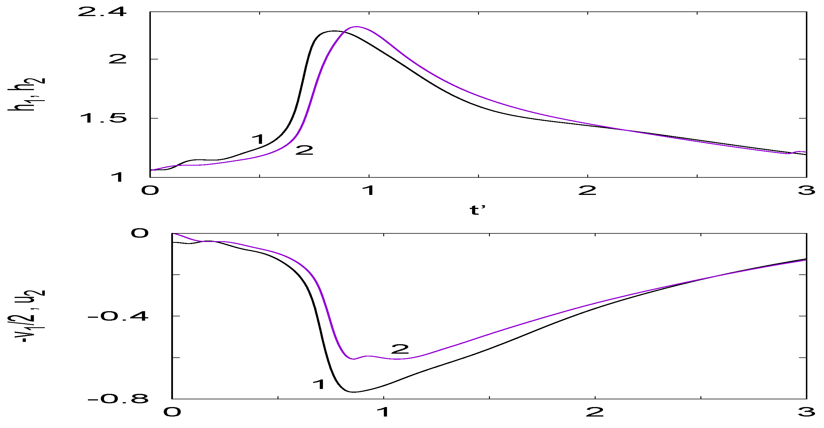
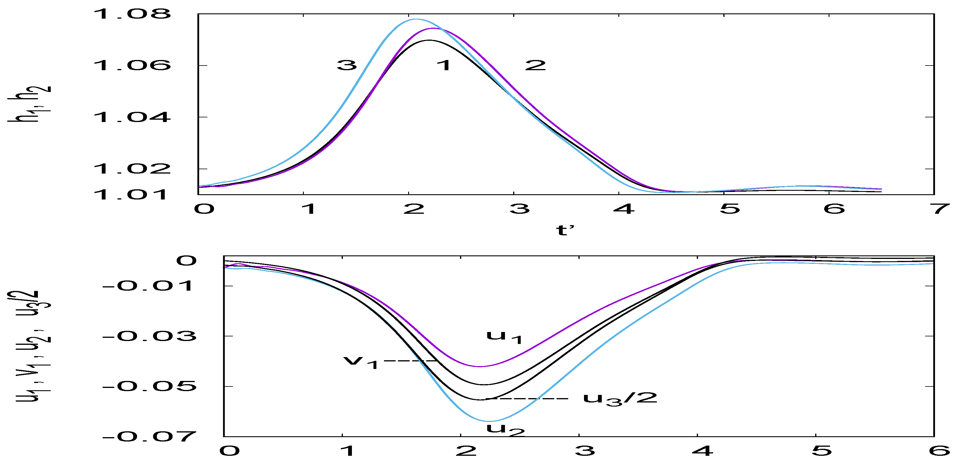
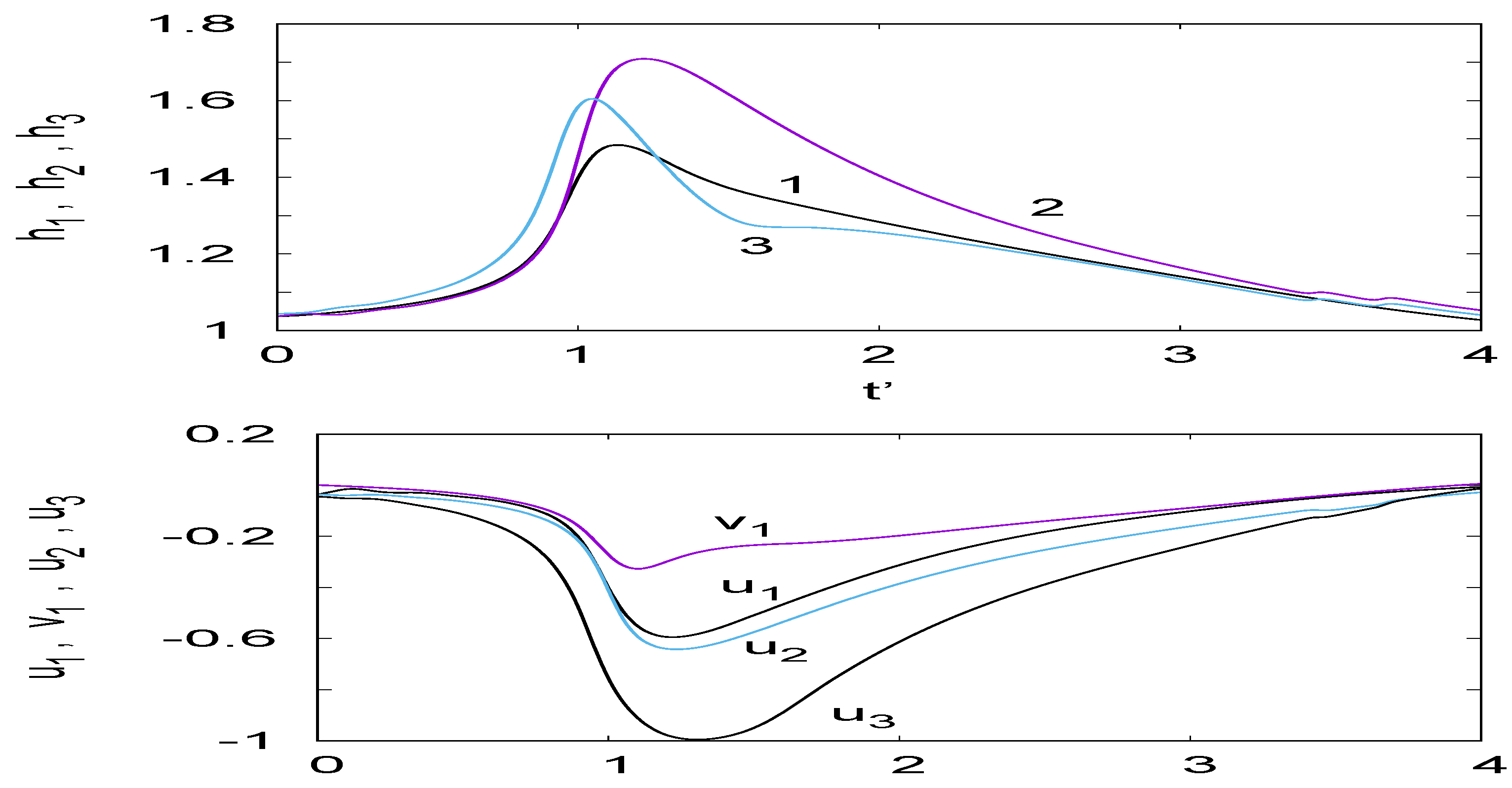
First observe that is non zero and close to . Nevertheless, the mass and energy residuals and are small as seen in Figure 12. The wave elevation h does not vary much from one branch to the other as seen in the top panel of Figure 13. The velocities and verify . These two results show that the Stoker conditions hold for this small amplitude.
5.2.2. Large Amplitude Waves
Figure 14 shows for a wave incident in branch 3 for . Notice the complex structure of the flow at the junction. There is some recirculation so that the flow is essentially 2D and not amenable to a 1D reduction.
Nevertheless, for a smaller amplitude , the balance laws (41)–(44) give some insight into the flow. Figure 15 shows the mass and energy . The mass is much better conserved than the energy.
When the wave is coming from branch 3, an obvious solution is
This is simplistic, in reality but remains small. The horizontal component is non zero and close to as shown in Figure 17.
The mass equation and y momentum equations allow to extract relations between . Assuming smaller than , we have
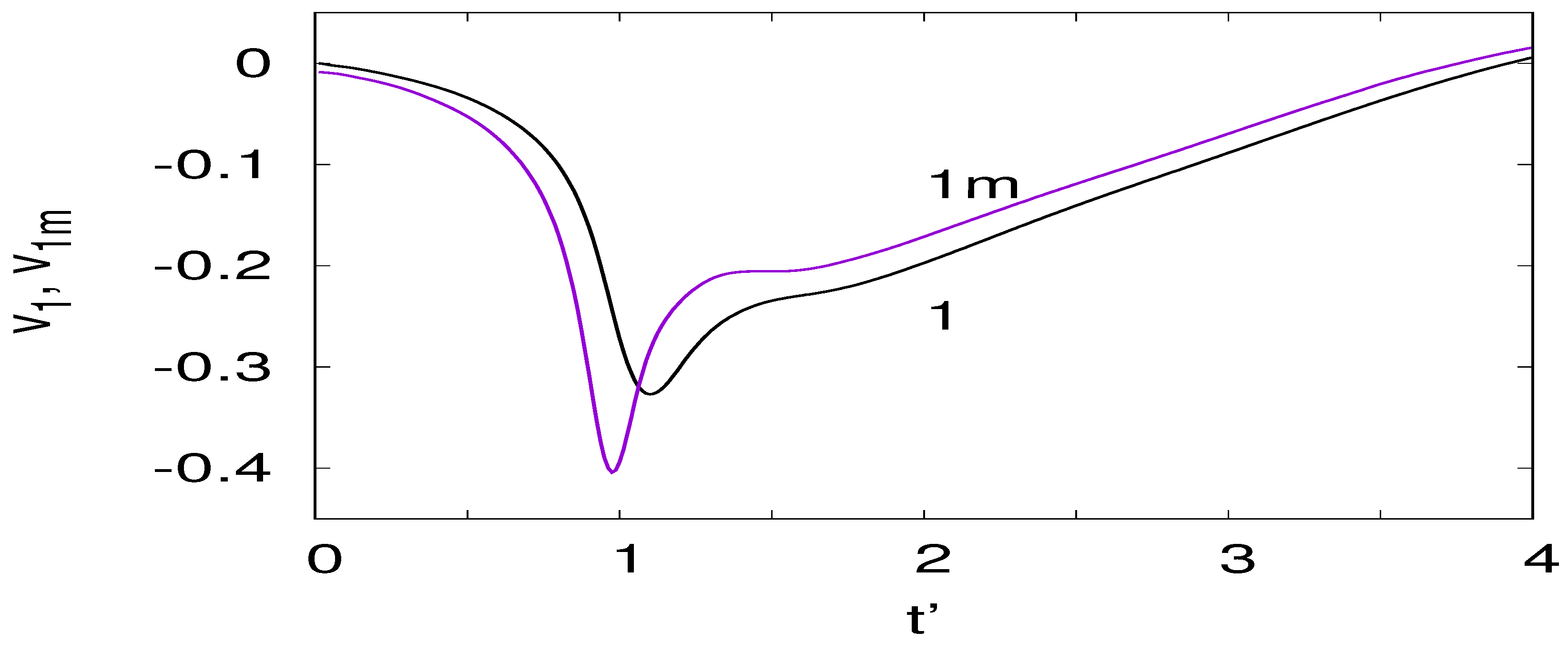
The quantity (34) in the y component of the momentum is computed from the numerical solution. It is plotted as a function of time together with the estimate
in the left panel of Figure 18. As can be seen, the agreement is very good.
The velocity given by the mass conservation relation agrees semi-quantitatively with the value estimated from the 2D numerical solution. Both quantities are plotted as a function of time in Figure 19. Note the delay due to the time the wave needs to propagate from one interface to the other. The y momentum conservation law is not satisfied so that there is no additional equation to estimate .
6. Discussion and Conclusions
The results of the previous section show that for large amplitudes and an asymmetric fork Stoker’s interface conditions do not hold and the angle of the fork plays a role. This seems to contradict the findings of Shi et al. [9]. Two reasons show that there is no contradiction. First, the amplitude of our waves () are much larger than the ones presented in [9] () so that nonlinear effects are much stronger in our study. The other point is that the initial condition is an exact solution of the Boussinesq equations, but not of the nonlinear shallow water equations. For the Boussinesq equations, we also expect an angle dependence, even for narrow channels, when the amplitude becomes large. To see this, we examine the reduction of the equations for a fork.
The Boussinesq equations read
where is the water elevation. The velocity potential is such that . The boundary conditions are non slip . Integrating the equations on the fork domain (left panel of Figure 1) we get
Neglecting the time evolution in the fork region, we get the following interface conditions
Note how the first equation reduces to Kirchhoff’s law for small h. The second equation contains is an integral over the whole domain and depends on the angle of the fork. For small angles, we can assume that so that the conditions reduce to
Not surprisingly, these conditions are very close to the ones obtained by Nachbin and Simoes [10], except for the Jacobian of the conformal transformation.
To conclude, we studied the propagation of shallow water waves in a fork between three narrow channels. We considered both the 2D numerical solution and a homothetic reduction procedure that gives coupling conditions at the interface. For such narrow widths, the delay experienced by the wave is negligible so that one can envision describing the junction by an effective 1D PDE model.
Our reduction enabled us to derive balance laws for the mass, momenta and energy of the flow across a general junction. For small amplitude waves, these laws reduce to the commonly used Stoker jump conditions, giving these a formal justification. We verified these Stoker conditions on the 2D numerical solutions of the shallow water equations for symmetric and non symmetric conditions. Then, the angle of the junction does not play any role. This happens also for a general nonlinear wave equation; we had seen this a previous study for the particular case of the sine-Gordon equation [2].
For large amplitude shallow water waves, the situation depends on the symmetry of the fork. For a symmetric fork, the Stoker conditions are approximately verified. This is explained by the strong constraint imposed by the symmetry. Then, the only solution of the balance laws corresponds to the Stoker conditions. When the fork is non symmetric as in our case 2, more information is needed about what happens inside the fork. The quantities are velocities projected in the direction of the branches and this projection leads to a loss of information. Far from the junction, the flow is quasi-1D so that not much is lost. On the contrary, inside the junction, the flow is full 2D. A possible solution, to be studied in the future would be to use the full conservation law including the time dependent term. Then we would introduce a fictitious node inside the junction and couple it to the boundaries using average differential equations obtained by integrating (9)–(11) on the fork domain.
Author Contributions
J.-G.C. calculated the conservation laws, analyzed the numerical data and wrote the manuscript. D.D. performed the 2D simulations of wave propagation across the fork with VOLNA code. He also participated in the analysis of the numerical results. B.G. studied the stucture of the conservation laws and the numerical results.
Funding
This research was funded by ANR grant “Fractal grid” and by the CNRS through the project PEPS InPhyNiTi “FARA”.
Acknowledgments
The authors thank Tim Minzoni and Nick Ercolani for useful discussions. We also thank the Centre Régional Informatique et d’Applications Numériques de Normandie for the use of its computers.
Conflicts of Interest
The authors declare no conflict of interest.
References
- Bressan, A.; Čanić, S.; Garavello, M.; Herty, M.; Piccoli, B. Flows on networks: Recent results and perspectives. EMS Surv. Math. Sci. 2014, 1, 47–111. [Google Scholar] [CrossRef]
- Caputo, J.-G.; Dutykh, D. Nonlinear waves in networks: model reduction for the sine-Gordon equation. Phys. Rev. E 2014, 90, 022912. [Google Scholar] [CrossRef] [PubMed]
- Hadamard, J. Leçons sur la géométrie élémentaire. Librairie Armand Colin 1906, 17, 103–209. [Google Scholar]
- Stoke, J.J. Water Waves: The Mathematical Theory with Applications; Wiley-Interscience: Hoboken, NJ, USA, 1992. [Google Scholar]
- Jacovkis, P.M. One-dimensional hydrodynamic flow in complex networks and some generalizations. Siam J. Appl. Math. 1991, 51, 948–966. [Google Scholar] [CrossRef]
- Holden, H.; Risebro, N.H. Riemann problems with a kink. Siam J. Appl. Math. 1999, 30, 497–515. [Google Scholar] [CrossRef]
- Landau, L.; Lifchitz, E. Cours de Physique Théorique: Hydrodynamique; Ellipses: Moscow, Russia, 1990. [Google Scholar]
- Georg Schmidt, E.J.P. On Junctions in a Network of Canals, In Control Theory of Partial Differential Equations; Chapman and Hall/CRC: Boca Raton, FL, USA, 2005; pp. 207–212. [Google Scholar]
- Shi, A.; Teng, M.H.; Sou, I.M. Propagation of long water waves through branching channels. J. Eng. Mech. 2005, 131, 859. [Google Scholar] [CrossRef]
- Nachbin, A.; Simoes, V.S. Solitary waves in forked channel regions. J. Fluid Mech. 2015, 777, 544–568. [Google Scholar] [CrossRef]
- Exner, P.; Post, O. Quantum networks modelled by graphs. AIP Conf. Proc. 2008, 998, 1. [Google Scholar]
- Post, O. Spectral Analysis on Graph-Like Spaces. In Lecture Notes in Mathematics; Springer: Berlin, Germany, 2012. [Google Scholar]
- Dutykh, D.; Caputo, J.-G. Wave dynamics on networks: Method and application to the sine-Gordon equation. Appl. Numer. Math. 2018, 131, 54–71. [Google Scholar] [CrossRef]
- Dutykh, D.; Katsaounis, T.; Mitsotakis, D. Finite volume schemes for dispersive wave propagation and runup. J. Comput. Phys. 2011, 230, 3035–3061. [Google Scholar] [CrossRef]
- Dutykh, D.; Poncet, R.; Dias, F. The VOLNA code for the numerical modeling of tsunami waves: Generation, propagation and inundation. Eur. J. Mech. B 2011, 30, 598–615. [Google Scholar] [CrossRef]
- Shampine, L.F.; Reichelt, M.W. The MATLAB ODE Suite. SIAM J. Sci. Comput. 1997, 18, 1–22. [Google Scholar] [CrossRef]
- Serre, F. Contribution à l’étude des écoulements permanents et variables dans les canaux. La Houille Blanche 1953, 8, 374–388; 830–872. [Google Scholar] [CrossRef]
- Dutykh, D.; Clamond, D.; Milewski, P.; Mitsotakis, D. Finite volume and pseudo-spectral schemes for the fully nonlinear 1D Serre equations. Eur. J. Appl. Math. 2013, 24, 761–787. [Google Scholar] [CrossRef]
Figure 1.
A fork geometry with arbitrary angles (left) and with right angles (right).

Figure 2.
Time evolution of the energies for the kink motion in branches for the T-junction (90 degrees) in full line (red online), for the Y-junction (45 degrees) in dashed line. The energy for the 1D effective model is plotted with points.
Figure 2.
Time evolution of the energies for the kink motion in branches for the T-junction (90 degrees) in full line (red online), for the Y-junction (45 degrees) in dashed line. The energy for the 1D effective model is plotted with points.

Figure 3.
Space discretization for the 1D approximation.

Figure 4.
Time evolution of the wave mass (left) and the wave energy (right) for a wave incident in branch 1 for .
Figure 4.
Time evolution of the wave mass (left) and the wave energy (right) for a wave incident in branch 1 for .

Figure 5.
Time evolution of the mass and energy quantities (black online) and (red online) for .

Figure 6.
Time evolution of (top) and (bottom) for .

Figure 7.
Snapshot of the surface elevation h at time for a wave incident in branch 1 for .

Figure 8.
Time evolution of the wave mass (left) and the wave energy (right) for a wave incident in branch 1 for .
Figure 8.
Time evolution of the wave mass (left) and the wave energy (right) for a wave incident in branch 1 for .

Figure 9.
Time evolution of the mass and energy quantities for .

Figure 10.
Time evolution of (top) and (bottom) for .

Figure 11.
Time evolution of the wave mass (left) and the wave energy (right) for a wave incident in branch 3 for (top panels) and (bottom panels). Notice the different scales.
Figure 11.
Time evolution of the wave mass (left) and the wave energy (right) for a wave incident in branch 3 for (top panels) and (bottom panels). Notice the different scales.

Figure 12.
Time evolution of the mass and energy quantities (black online) and (red online) for .

Figure 13.
Time evolution of and (top) and (bottom) for .

Figure 14.
Snapshot of the surface elevation h at time for a wave incident in branch 3 for .

Figure 15.
Time evolution of the mass and energy quantities (black online) and (purple online) for .
Figure 15.
Time evolution of the mass and energy quantities (black online) and (purple online) for .

Figure 16.
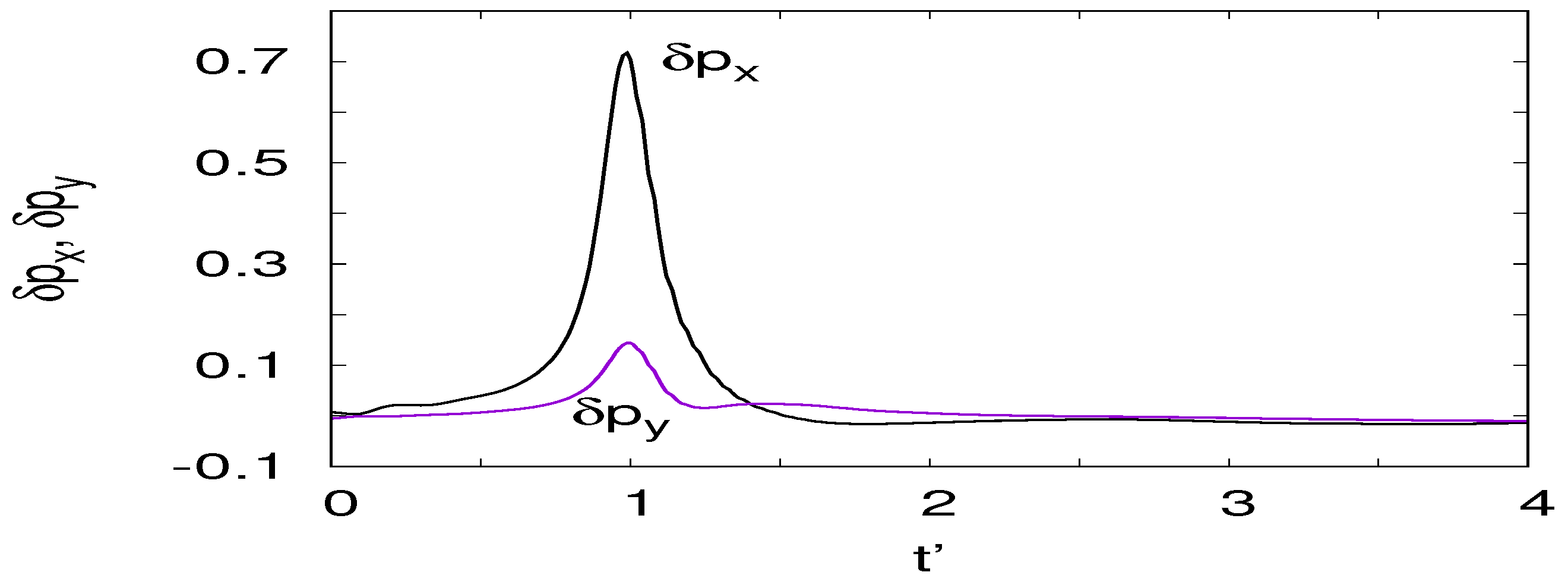
Time evolution of the x and y momenta quantities (black online) and (purple online) for .
Figure 16.
Time evolution of the x and y momenta quantities (black online) and (purple online) for .

Figure 17.
Time evolution of (top) and (bottom) for .

Figure 18.
(Left) panel, time evolution of the quantity (purple online) from (34) obtained from the 2D numerics together with the approximation (51) (black online) indicated by the * symbol. (Right) panel, time evolution of and .

Figure 19.
Time evolution of the quantity obtained from the mass conservation law (49) (purple online) and from the 2D numerical solution (black online).
Figure 19.
Time evolution of the quantity obtained from the mass conservation law (49) (purple online) and from the 2D numerical solution (black online).


Table 1.
The two different dynamic problems for the T-branch.
| Type | Known | Unknown |
|---|---|---|
| wave in branch 1 | ||
| wave in branch 3 |
© 2019 by the authors. Licensee MDPI, Basel, Switzerland. This article is an open access article distributed under the terms and conditions of the Creative Commons Attribution (CC BY) license (http://creativecommons.org/licenses/by/4.0/).
Share and Cite
MDPI and ACS Style
Caputo, J.; Dutykh, D.; Gleyse, B. Coupling Conditions for Water Waves at Forks. Symmetry 2019, 11, 434. https://doi.org/10.3390/sym11030434
AMA Style
Caputo J, Dutykh D, Gleyse B. Coupling Conditions for Water Waves at Forks. Symmetry. 2019; 11(3):434. https://doi.org/10.3390/sym11030434
Chicago/Turabian StyleCaputo, Jean–Guy, Denys Dutykh, and Bernard Gleyse. 2019. "Coupling Conditions for Water Waves at Forks" Symmetry 11, no. 3: 434. https://doi.org/10.3390/sym11030434
Note that from the first issue of 2016, this journal uses article numbers instead of page numbers. See further details here.