Cosmological Consequences of New Dark Energy Models in Einstein-Aether Gravity


1
Department of Mathematics, COMSATS University Islamabad, Lahore-Campus, Lahore 54000, Pakistan
2
Division of Human Support System, Faculty of Symbiotic Systems Science, Fukushima University, Fukushima 960-1296, Japan
3
Allied School, Ali Campus, Muhafiz Town Canal Road, Lahore 54000, Pakistan
*
Author to whom correspondence should be addressed.
Symmetry 2019, 11(4), 509; https://doi.org/10.3390/sym11040509
Submission received: 16 February 2019
/
Revised: 18 March 2019
/
Accepted: 28 March 2019
/
Published: 8 April 2019
(This article belongs to the Special Issue Cosmological Inflation, Dark Matter and Dark Energy)
Abstract
:In this paper, we reconstruct various solutions for the accelerated universe in the Einstein-Aether theory of gravity. For this purpose, we obtain the effective density and pressure for Einstein-Aether theory. We reconstruct the Einstein-Aether models by comparing its energy density with various newly proposed holographic dark energy models such as Tsallis, Rényi and Sharma-Mittal. For this reconstruction, we use two forms of the scale factor, power-law and exponential forms. The cosmological analysis of the underlying scenario has been done by exploring different cosmological parameters. This includes equation of state parameter, squared speed of sound and evolutionary equation of state parameter via graphical representation. We obtain some favorable results for some values of model parameters
1. Introduction
Nowadays, it is believed that our universe is undergoing an accelerated expansion with the passage of cosmic time. This cosmic expansion has been confirmed through various observational schemes such as supernova type Ia (SNIa) [1,2,3,4] and the cosmic microwave background (CMB) [5,6,7,8,9]. The source behind the expansion of the universe is a mysterious force called dark energy (DE) and its nature is still ambiguous [10,11,12,13]. The current Planck data shows that DE accounts for of the total energy contents of the universe. The first candidate for describing the DE phenomenon is the cosmological constant but it has fine tuning and cosmic coincidence problems. Due to this reason, different DE models as well as theories of gravity with modifications have been suggested. The dynamical DE models include a family of Chaplygin gas as well as holographic DE models, scalar field models such as K-essence, phantom, quintessence, ghost, etc. [14,15,16,17,18,19,20,21,22,23,24,25,26].
One of the DE model is the holographic DE (HDE) model which becomes a favorable technique now-a-days to study the DE mystery. This model is established in the framework of holographic principle which corresponds to the area instead of volume for the scaling of the number of degrees of freedom of a system. This model is an interesting effort in exploring the nature of DE in the framework of quantum gravity. In addition, the HDE model gives the relationship between the energy density of quantum fields in vacuum (as the DE candidate) to the cutoffs (infrared and ultraviolet). Cohen et al. [27] provided a very useful result about the expression of the HDE model density which is based on the vacuum energy of the system. The black hole mass should not be overcome by the maximum amount of the vacuum energy. Taking into account the nature of spacetime along with long term gravity, various entropy formalisms have been used to discuss the gravitational and cosmological setups [28,29,30,31,32,33]. Recently, some new HDE models are proposed, like Tsallis HDE (THDE) [31], Rényi HDE model (RHDE) [32] and Sharma-Mittal HDE (SMHDE) [33].
The examples of theories with modification setups include , etc., where R shows the Ricci scalar representing the curvature, T means the torsion scalar, is the trace of the energy-momentum tensor and G goes as the invariant of Gauss–Bonnet [34,35,36,37,38,39,40,41,42,43,44,45]. For recent reviews in terms of DE problems including modified gravity theories, see, for instance [46,47,48,49,50,51,52]. The Einstein-Aether theory is one of the modified theories of gravity [53,54] and accelerated expansion phenomenon of the universe has also been investigated in this theory [55]. Meng et al. have also discussed the current cosmic acceleration through DE models in this gravity [56,57]. Recently, Pasqua et al. [58] have made versatile studies on cosmic acceleration through various cosmological models in the presence of HDE models.
In the present work, we will develop the Einstein-Aether gravity models in the presence of modified HDE models and well-known scale factors. For these models of modified gravity, we will extract various cosmological parameters. In the next section, we will give a brief review of the Einstein-Aether theory. In Section 3, we present the basic cosmological parameters as well as well-known scale factors. We will discuss the cosmological parameters for modfied HDE models in Section 4, Section 5 and Section 6. In the last section, we will summarize our results.
2. Einstein-Aether Theory
As our universe is full with many of the natural occurring phenomenons. One of them is transfer of light from one place to another and second is how gravity acts. To explain these kinds of phenomenons, many of the physicists were used the concept of Aether in many of the theories. In modern physics, Aether indicates a physical medium that is spread homogeneously at each point of the universe. Hence, it was considered that it is a medium in space that helps light to travel in a vacuum. According to this concept, a particular static frame reference is provided by Aether and everything has absolute relative velocity in this frame. That is suitable for Newtonian dynamics extremely well. But, when Einstein performed different experiments on optics in his theory of relativity, then Einstein rejected this ambiguity. When CMB was introduced, many of the people took it a modern form of Aether. Gasperini has popularized Einstein-Aether theories [59]. This theory is said to be covariant modification of general relativity in which unit time like vector field(aether) breaks the Lorentz Invariance (LI) to examine the gravitational and cosmological effects of dynamical preferred frame [53]. Following is the action of Einstein-Aether theory [60,61].
where represents the Lagrangian density for the vector field and indicates Lagrangian density of matter field. Further, and G indicate determinant of the metric tensor , Ricci scalar and gravitational constant respectively. The Lagrangian density for vector field can be written as
where represents a Lagrangian multiplier, dimensionless constants are denoted by referred as coupling constant parameter and is a tensor of rank one, that is a vector. The function is any arbitrary function of K. We obtain the Einstein field equations from Equation (1) for the Einstein-Aether theory as follows
where shows energy momentum-tensor for vector field and indicates energy-momentum tensor for mater field. These tensors are given as
where p and represent energy density and pressure of the matter respectively. Furthermore, expresses the four-velocity vector of the fluid and given as and is time-like unitary vector and is defined as . Moreover is defined as
where indices show the symmetry.
The Friedmann equations modified by the Einstein-Aether gravity are given as follows
3. Cosmological Parameters
To understand the geometry of the universe, the following are some basic cosmological parameters.
3.1. Equation of State Parameter
In order to categorize the different phases of the evolving universe, the EoS parameter is widely used. In particular, the decelerated and accelerated phases contain DE, DM, radiation dominated eras. This parameter is defined in terms of energy density and pressure p as .
- In the decelerated phase, the radiation era and cold DM era are included.
- The accelerated phase of the universe has following eras: cosmological constant, quintessence and phantom era of the universe.
3.2. Squared Speed of Sound
To examine the behavior of DE models, there is another parameter which is known as squared speed of sound. It is denoted by and is calculated by the following formula
The stability of the model can be checked by this relation. If its graph is showing negative values then we may say that model is unstable and in case of non-negative values of the graph, it represents the stable behavior of the model.
3.3. - Plane
There are different DE models which have different properties. To examine their dynamical behavior, we use - plane, where prime denotes the derivative with respect to and subscript indicates DE scenario. This method was developed by Caldwell and Linder [62] and divides - plane into two parts. One is the freezing part in which evolutionary parameter gives negative behavior for negative EoS parameter, i.e., , while for positive behavior of evolutionary parameter corresponding to negative EoS parameter yields the thawing part () of the evolving universe.
3.4. Scale Factor
The scale factor is the measure of how much the universe has expanded since a given time. It is represented by . Since the latest cosmic observations have shown that the universe is accelerating so . As Einstein-Aether is one of the modified theory which may produce the accelerated expansion of the universe, by using this theory, we can reconstruct various well-known DE models. In order to do this, we take some modified HDE models such as THDE, RHDE and SMHDE models. Since is a function that the Einstein-Aether theory contains, which can be determined by comparing the densities with the above DE models. For this purpose, we use some well-known forms of the scale factor, . We consider two forms of scale factors in terms of power and exponential terms. These are
4. Reconstruction from the Tsallis Holographic Dark Energy Model
The energy density of THDE model is given by [31]
where B is an unknown parameter. Taking into account Hubble radius as IR cutoff L, that is , we have
In order to construct a DE model in the framework of Einstein-Aether gravity with THDE model, we compare the densities of both models, (i.e., ). This yields
which results the following form
Power-law form of scale factor:
Using the expression of along with Equation (19) in (14), we obtain the energy density and pressure as
Using these expressions of energy density and pressure, we find the values of some cosmological parameters in the following. The EoS parameter takes the following form
The derivative of EoS parameter with respect to is given by
We plot the EoS parameter versus z using the relation taking values of constants as and . We plot for three different values of scale factor parameter m as as shown in Figure 1. All the three trajectories represent the phantom behavior of the universe related to the redshift parameter. In Figure 2, we plot plane taking same values of the parameters for . For and 3, the evolving EoS parameter shows negative behavior with respect to negative EoS parameter which indicates the freezing region of the universe. The trajectory of for represents the positive behavior for negative EoS parameter and expresses the evolving universe in thawing region of the universe.
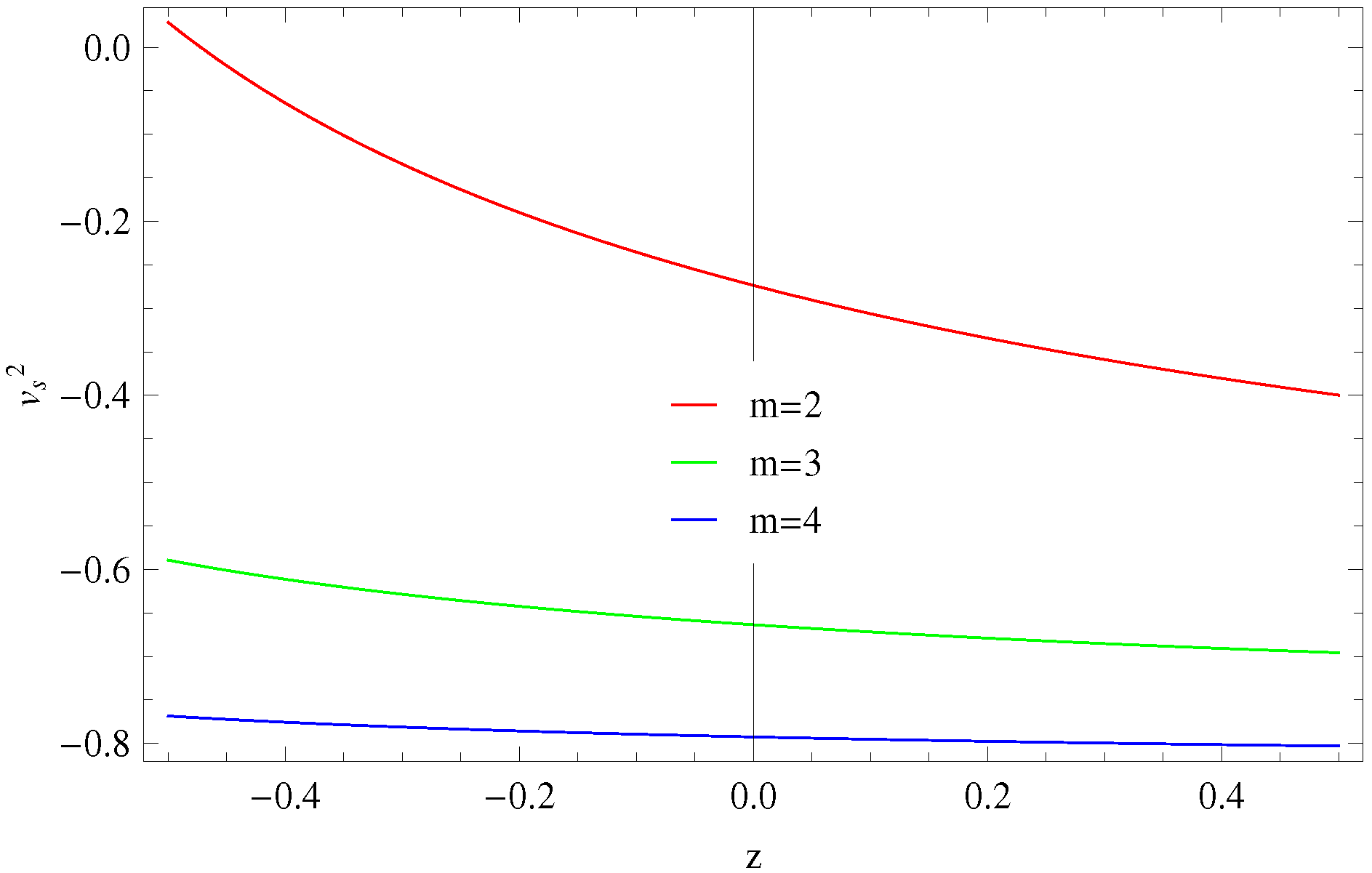
Also the squared speed of sound in the underlying scenario becomes
Figure 3 shows the plot of versus z to check the behavior of the Einstein-Aether model for the THDE and power-law scale factor for same values of parameters. The trajectories represent the negative behavior of the model which indicated the instability of the model.
Exponential form of scale factor:
Following the same steps for the exponential form of the scale factor, we get energy density and pressure as
Now, by using the above density and pressure, we obtain the EoS parameter and its derivative for the Einstein-Aether gravity as follows
The squared speed of sound for the second form of the scale factor is given by
Figure 4 represents the graph of the EoS parameter versus z for the exponential form of the scale factor taking and scale factor parameter . This parameter represents the phantom behavior of the universe for and after a transition from quintessence to phantom era for . For , the trajectory of the EoS parameter corresponds to the -CDM model . In Figure 5, the graph is plotted between and . The graph represents initially freezing region and then indicates the thawing region of the evolving universe. As we increase the value of , the trajectories indicate the thawing region only. However, the graph of versus z as shown in Figure 6 shows the unstable behavior.
5. Reconstruction from Rényi Holographic Dark Energy Model
The energy density of the RHDE model is [33]
For the Hubble horizon, it takes the form
Now we compare the Einstein-Aether model energy density with the RHDE model density (i.e., ) in order to get the reconstructed equation,
The solution of this equation is given by
Power-law form of the scale factor:
Inserting all the corresponding values into Equations (14) and (15), we get density and pressure of the Einstein-Aether gravity model as follows
In this case, the EoS parameter takes the form
and is given as follows
The expression for squared speed of sound turns out as
The plot of the EoS parameter is shown in Figure 7 with respect to z. All the trajectories of the EoS parameter represent the quintessence phase of the universe. Figure 8 shows the graph of plane for same range of z. The trajectories of describe the negative behavior for all give the freezing region of the universe. To check the stability of the underlying model, Figure 9 shows the unstable behavior of the model. However, for , we get some stable points for .
Exponential form of scale factor:
Taking into account second scale factor Equation (15) along with , we get the following energy density and pressure
The EoS parameter is obtained from the above energy density and pressure. This parameter with its derivative are given by
The correspond expression for is given by
Figure 10 represents the graph of the EoS parameter versus z for the RHDE model taking an exponential form of the scale factor. For , initially the trajectory expresses the transition from decelerated phase to accelerated phase and then crosses the phantom divide line and gives the phantom phase of the universe. For higher values of the , that is for , the trajectories of the EoS parameter represents the quintessence phase. In Figure 11, we plot the graph of evolution parameter of EoS versus EoS parameter which gives the freezing region of the universe. Figure 12 shows the graph of for stability analysis of the model. Initially the graph gives the stability and then for decreasing z, the model becomes unstable. As we increase the value of , the trajectories give more stable points.
6. Reconstruction from the Sharma-Mittal Holographic Dark Energy Model
Sharma-Mittal introduced two parametric entropy and defined it as [32]
where r is a new free parameter. The expression of the SMHDE model for the Hubble horizon is given by
By comparing the energy densities of the SMHDE model and Einstein-Aether gravity model, we find
which leads us to the following solution
Power-law form of scale factor:
For this scale factor, we obtain
The cosmological parameters are given by
We plot the EoS parameter for the SMHDE model with respect to the redshift parameter as shown in Figure 13 for the power-law scale factor. For and 4, the trajectories represent the transition from quintessence to phantom phase while indicates the phantom era throughout for z. The plot of this parameter with its evolution parameter is given in Figure 14, which shows the freezing region of the evolving universe. However, for higher values of m, we may get thawing region . Figure 15 gives the graph of squared speed of sound versus redshift. The trajectory for shows the stability of the model as redshift parameter decreases while other trajectories describe the unstable behavior of the model.
Exponential form of scale factor:
Following the same steps, we obtain the following expressions for energy density, pressure and parameters for exponential scale factor. These are:
For the exponential scale factor for the SMHDE model, the plot of the EoS parameter in Figure 16 represents the phantom behavior initially, but converges to the cosmological constant behavior for , as z decreases. For , the EoS parameter gives the phantom behavior. Figure 17 represents the graph of the plane, which shows the positive behavior of versus negative expressing thawing region of the universe. The squared speed of sound graph gives unstable behavior of the SMHDE model in the framework of the Einstein-Aether theory of gravity as shown in Figure 18.
7. Summary
In this work, we have discussed Einstein-Aether gravity and utilized its effective density and pressure. We have developed the Einstein-Aether models by using some holographic dark energy models. In the presence of a free function , we have treated the affective density and pressure as DE. From the modified HDE models such as the THDE, RHDE and SMHDE models, we have formed the unknown function for the Einstein-Aether theory by considering the power-law form and exponential forms of scale factor. We have discussed some cosmological parameters, like the EoS parameter with its evolutionary parameter and squared speed of sound to check the stability of the reconstructed models for this theory.
The remaining results have been summarized as follows:
- EoS parameter for power-law scale factor:
- THDE ⇒ phantom behavior,
- RHDE ⇒ quintessence phase,
- SMHDE ⇒ transition from quintessence to phantom phase for , phantom era for .
- EoS parameter for exponential scale factor:
- THDE ⇒ transition from quintessence to phantom era for , phantom behavior for , CDM model for ,
- RHDE ⇒ phantom phase for , quintessence phase for
- SMHDE ⇒ cosmological constant behavior for , phantom behavior for .
- - plane for power-law scale factor:
- THDE ⇒ freezing region for , thawing region for ,
- RHDE ⇒ freezing region,
- SMHDE ⇒ freezing region.
- - plane for exponential scale factor:
- THDE ⇒ freezing region to thawing region,
- RHDE ⇒ freezing region,
- SMHDE ⇒ thawing region.
- Squared speed of sound for power-law scale factor:
- THDE ⇒ unstable,
- RHDE ⇒ unstable,
- SMHDE ⇒ stable for , unstable for .
- Squared speed of sound for exponential scale factor:
- THDE ⇒ unstable,
- RHDE ⇒ stability for higher values and instability for lower values,
- SMHDE ⇒ unstable.
It is mentioned here that for for the power-law form of the scale factor in the case of the SMHDE model, we obtain a phantom region with stable behavior in the freezing region which leads to the most favorable result within the current cosmic expansion scenario.
Author Contributions
A.J. and S.R. proposed and completed the draft of the paper, K.B. done the proof reading and I.U.M. contributed in the mathematical work of the manuscript.
Funding
This research received no external funding.
Acknowledgments
S.R. and A.J. are thankful to the Higher Education Commission, Islamabad, Pakistan for its financial support under the grant No: 5412/Federal/NRPU/R&D/HEC/2016 of NATIONAL RESEARCH PROGRAMME FOR UNIVERSITIES (NRPU). The work of KB was partially supported by the JSPS KAKENHI Grant Number JP 25800136 and Competitive Research Funds for Fukushima University Faculty (18RI009).
Conflicts of Interest
The authors declare no conflict of interest.
References
- Komatsu, E.; Dunkley, J.; Nolta, M.R.; Bennett, C.L.; Gold, B.; Hinshaw, G.; Jarosik, N.; Larson, D.; Limon, M.; Page, L.; et al. Five-year Wilkinson Microwave Anisotropy probe Observations: Cosmological Interpretation. Astrophys. J. Suppl. 2009, 180, 330–376. [Google Scholar] [CrossRef]
- Nolta, M.R.; Dunkley, J.; Hill, R.S.; Hinshaw, G.; Komatsu, E.; Larson, D.; Page, L.; Spergel, D.N.; Bennett, C.L.; Gold, B.; et al. Five-year Wilkinson Microwave Anisotropy probe Observations: Angular Power Spectra. Astrophys. J. Suppl. 2009, 180, 296–305. [Google Scholar] [CrossRef]
- Bahcall, N.; Ostriker, J.P.; Perlmutter, S.; Steinhardt, P.J. The Cosmic Triangle: Revealing the State of the Universe. Science 1999, 284, 1481–1488. [Google Scholar] [CrossRef]
- Perlmutter, S.; Aldering, G.; Goldhaber, G.; Knop, R.A.; Nugent, P.; Castro, P.G.; Deustua, S.; Fabbro, S.; Goobar, A.; Groom, D.E.; et al. Measurements of Omega and Lambda from 42 High-Redshift Supernovae. APJ 1999, 517, 565–586. [Google Scholar] [CrossRef]
- Perlmutter, S.; Aldering, G.; Valle, M.D.; Deustua, S.; Ellis, R.S.; Fabbro, S.; Fruchter, A.; Goldhaber, G.; Goobar, A.; Groom, D.E.; et al. Discovery of a Supernova Explosion at Half the Age of the Universe and its Cosmological Implications. Nature 1998, 391, 51–54. [Google Scholar] [CrossRef]
- Riess, A.G.; Filippenko, A.V.; Challis, P.; Clocchiattia, A.; Diercks, A.; Garnavich, P.M.; Gilliland, R.L.; Hogan, C.J.; Jha, S.; Kirshner, R.P.; et al. Observational Evidence from Supernovae for an Accelerating Universe and a Cosmological Constant. Astron. J. 1998, 116, 1009–1038. [Google Scholar] [CrossRef]
- Riess, A.G.; Strolger, L.G.; Tonry, J.; Casertano, S.; Ferguson, H.C.; Mobasher, B.; Challis, P.; Filippenko, A.V.; Jha, S.; Li, W.; et al. Type Ia Supernova Discoveries at z > 1 from the Hubble Space Telescope: Evidence for Past Deceleration and Constraints on Dark Energy Evolution. Astrophys. J. 2004, 607, 665–687. [Google Scholar] [CrossRef]
- Boisseau, B.; Esposito-Farese, G.; Polarski, D.; Starobinsky, A.A. Reconstruction of a Scalar-Tensor Theory of Gravity in an Accelerating Universe. Phys. Rev. Lett. 2000, 85, 2236. [Google Scholar] [CrossRef] [PubMed]
- Spergel, D.N.; Bean, R.; Dore, O.; Nolta, M.R.; Bennett, C.L.; Dunkley, J.; Hinshaw, G.; Jarosik, N.; Komatsu, E.; Page, L.; et al. Wilkinson Microwave Anisotropy Probe (WMAP) Three Year Results: Implications for Cosmology. Astrophys. J. Suppl. Ser. 2007, 170, 377. [Google Scholar] [CrossRef]
- Gardner, C.L. Quintessence and the Transition to an Accelerating Universe. Nucl. Phys. B 2005, 707, 278. [Google Scholar] [CrossRef]
- De Leon, J.P. Transition from Decelerated to Accelerated Cosmic Expansion in Braneworld Universes. Gen. Relativ. Gravit. 2006, 38, 61–81. [Google Scholar] [CrossRef]
- Cunha, J.V. Kinematic Constraints to the Transition Redshift from Supernovae Type Ia Union Data. Phys. Rev. D 2009, 79, 047301. [Google Scholar] [CrossRef]
- Roos, M. Introduction to Cosmology; John Wiley and Sons: Chichester, UK, 2003. [Google Scholar]
- Jawad, A.; Majeed, A. Ghost Dark Energy Models in Specific Modified Gravity. Astrophy. Space Sci. 2015, 356, 375. [Google Scholar] [CrossRef]
- Jawad, A. Cosmological Analysis of Pilgrim Dark Energy in Loop Quantum Cosmology. Eur. Phys. J. C 2015, 75, 206. [Google Scholar] [CrossRef]
- Jawad, A.; Chattopadhyay, S.; Pasqua, A. A Holographic Reconstruction of the Modified f(R) Horava-Lifshitz Gravity with Scale Factor in Power-law form. Astrophy. Space Sci. 2013, 346, 273. [Google Scholar] [CrossRef]
- Jawad, A.; Chattopadhyay, S.; Pasqua, A. Reconstruction of f(G) Gravity with the New Agegraphic Dark-energy Model. Eur. Phys. J. Plus 2013, 128, 88. [Google Scholar] [CrossRef]
- Jawad, A.; Chattopadhyay, S.; Pasqua, A. Reconstruction of f() models via well-known scale factors. Eur. Phys. J. Plus 2014, 129, 54. [Google Scholar] [CrossRef]
- Jawad, A.; Pasqua, A.; Chattopadhyay, S. Correspondence between f(G) gravity and holographic dark energy via power-law solution. Astrophy. Space Sci. 2013, 344, 489. [Google Scholar] [CrossRef]
- Jawad, A.; Pasqua, A.; Chattopadhyay, S. Holographic reconstruction of f(G) gravity for scale factors pertaining to emergent, logamediate and intermediate scenarios. Eur. Phys. J. Plus 2013, 128, 156. [Google Scholar] [CrossRef]
- Jawad, A. New Agegraphic Pilgrim Dark Energy in f(T,TG) Gravity. Astrophy. Space Sci. 2014, 353, 691. [Google Scholar] [CrossRef]
- Jawad, A.; Iqbal, A. Modified Cosmology through Renyi and logarithmic Entropies. Int. J. Geom. Meth. Mod. Phys. 2018, 15, 1850130. [Google Scholar] [CrossRef]
- Jawad, A.; Iqbal, A. Cosmological Implications of Non-canonical Scalar Field Model in Fractal Universe. Phys. Dark Univ. 2018, 22, 16–26. [Google Scholar] [CrossRef]
- Iqbal, A.; Jawad, A. Thermodynamics of Ricci-Gauss-Bonnet Dark Energy. Adv. High Energy Phys. 2018, 2018, 6139430. [Google Scholar] [CrossRef]
- Jawad, A.; Bamba, k.; Younas, M.; Qummer, S.; Rani, S. Tsallis, Rényi and Sharma-Mittal Holographic Dark Energy Models in Loop Quantum Cosmology. Symmetry 2018, 10, 635. [Google Scholar] [CrossRef]
- Younas, M.; Jawad, A.; Qummer, S.; Moradpour, H.; Rani, S. Cosmological Implications of the Generalized Entropy Based Holographic Dark Energy Models in Dynamical Chern-Simons Modified Gravity. Adv. High Energy Phys. 2019, 2019, 1287932. [Google Scholar] [CrossRef]
- Kaplan, D.B.; Nelson, A.E. Effective Field Theory, Black Holes, and the Cosmological Constant. Phys. Rev. Lett. 1999, 73, 4971–4974. [Google Scholar]
- Moradpour, H.; Sheykhi, A.; Corda, C.; Salako, I.G. Energy Definition and Dark Energy: A Thermodynamic Analysis. Phys. Lett. B 2018, 783, 82. [Google Scholar] [CrossRef]
- Moradpour, H.; Bonilla, A.; Abreu, E.M.C.; Neto, J.A. Einstein and Rastall Theories of Gravitation in Comparison. Phys. Rev. D 2017, 96, 123504. [Google Scholar] [CrossRef]
- Moradpour, H. Necessity of Dark Energy from Thermodynamic Arguments. Int. J. Theor. Phys. 2016, 55, 4176. [Google Scholar] [CrossRef]
- Tavayef, M.; Sheykhi, A.; Bamba, K.; Moradpour, H. Tsallis holographic dark energy. Phys. Lett. B 2018, 781, 195. [Google Scholar] [CrossRef]
- Moosavi, S.A.; Lobo, I.P.; Morais Graca, J.P.; Jawad, A.; Salako, I.G. Thermodynamic approach to holographic dark energy and the Rényi entropy. arXiv 2018, arXiv:1803.02195. [Google Scholar]
- Moosavi, S.A.; Moradpour, H.; Morais Graça, J.P.; Lobo, I.P.; Salako, I.G.; Jawad, A. Generalized entropy formalism and a new holographic dark energy model. Phys. Lett. B 2018, 780, 21–24. [Google Scholar]
- Nojiri, S.; Odintsov, S.D. Modified non-local-F(R) gravity as the key for the inflation and dark energy. Phys. Lett. B 2008, 659, 821–826. [Google Scholar] [CrossRef]
- Li, B.; Barrow, J.D. Cosmology of f(R) gravity in the metric variational approach. Phys. Rev. D 2007, 75, 084010. [Google Scholar] [CrossRef]
- Nojiri, S.; Odintsov, S.D. Modified f(R) gravity consistent with realistic cosmology: From matter dominated epoch to dark energy universe. Phys. Rev. D 2006, 74, 086005. [Google Scholar] [CrossRef]
- Dunsby, P.K.S.; Elizalde, E.; Goswami, R.; Odintsov, S.; Gomez, D.S. On the LCDM universe in f(R) gravity. Phys. Rev. D 2010, 82, 023519. [Google Scholar] [CrossRef]
- Elizalde, E.; Odintsov, S.D.; Pozdeeva, E.O.; Yu, S.; Vernov, J. Cosmological attractor inflation from the RG-improved Higgs sector of finite gauge theory. J. Cosmo. Astropart. Phys. 2016, 1602, 25. [Google Scholar] [CrossRef]
- Abdalla, M.C.B.; Nojiri, S.; Odintsov, S.D. Consistent modified gravity: Dark energy, acceleration and the absence of cosmic doomsday. Class. Quantum Gravity 2005, 22, L35. [Google Scholar] [CrossRef]
- Linder, E.V. Einstein’s other gravity and the acceleration of the Universe. Phys. Rev. D 2010, 81, 127301. [Google Scholar] [CrossRef]
- Yerzhanov, K.K. Emergent Universe in Chameleon, f(R) and f(T) Gravity Theories. arXiv 2010, arXiv:1006.3879v1. [Google Scholar]
- Nojiri, S.; Odintsov, S.D. Modified Gauss-Bonnet theory as gravitational alternative for dark energy. Phys. Lett. B 2005, 631, 1–6. [Google Scholar] [CrossRef]
- Antoniadis, I.; Rizos, J.; Tamvakis, K. Singularity-free cosmological solutions of the superstring effective action. Nucl. Phys. B 1994, 415, 497–514. [Google Scholar] [CrossRef]
- Horava, P. Membranes at Quantum Criticality. JHEP 2009, 903, 20. [Google Scholar] [CrossRef]
- Brans, C.; Dicke, H. Mach’s Principle and a Relativistic Theory of Gravitation. Phys. Rev. 1961, 124, 925. [Google Scholar] [CrossRef]
- Nojiri, S.; Odintsov, S.D. Unified cosmic history in modified gravity: From F(R) theory to Lorentz non-invariant models. Phys. Rep. 2011, 505, 59–144. [Google Scholar] [CrossRef]
- Capozziello, S.; de Laurentis, M. Extended Theories of Gravity. Phys. Rep. 2011, 509, 167–321. [Google Scholar] [CrossRef]
- Faraoni, V.; Capozziello, S. Beyond Einstein Gravity: A Survey of Gravitational Theories for Cosmology and Astrophysics; Springer: Dordrecht, The Netherlands, 2011. [Google Scholar]
- Bamba, K.; Odintsov, S.D. Inflationary cosmology in modified gravity theories. Symmetry 2015, 7, 220–240. [Google Scholar] [CrossRef]
- Cai, Y.F.; Capozziello, S.; de Laurentis, M.; Saridakis, E.N. f(T) teleparallel gravity and cosmology. Rep. Prog. Phys. 2016, 79, 106901. [Google Scholar] [CrossRef]
- Nojiri, S.; Odintsov, S.D.; Oikonomou, V.K. Modified Gravity Theories on a Nutshell: Inflation, Bounce and Late-time Evolution. Phys. Rep. 2017, 692, 1–104. [Google Scholar] [CrossRef]
- Bamba, K.; Capozziello, S.; Nojiri, S.; Odintsov, S.D. Dark energy cosmology: The equivalent description via different theoretical models and cosmography tests. Astrophys. Space Sci. 2012, 342, 155–228. [Google Scholar] [CrossRef]
- Jacobson, T.; Mattingly, D. Gravity with a dynamical preferred frame. Phys. Rev. D 2001, 64, 024028. [Google Scholar] [CrossRef]
- Jacobson, T.; Mattingly, D. Einstein-aether waves. Phys. Rev. D 2004, 70, 024003. [Google Scholar] [CrossRef]
- Barrow, J.D. Errata for cosmological magnetic fields and string dynamo in axion torsioned spacetime. Phys. Rev. D 2012, 85, 047503. [Google Scholar] [CrossRef]
- Meng, X.; Du, X. Einstein-aether theory as an alternative to dark energy model. Phys. Lett. B 2012, 710, 493–499. [Google Scholar] [CrossRef]
- Meng, X.; Du, X. A Specific Case of Generalized Einstein-aether Theories. Commun. Theor. Phys. 2012, 57, 227. [Google Scholar] [CrossRef]
- Achucarro, A.; Gong, J.O.; Hardeman, S.; Palma, G.A.; Patil, S.P. Features of heavy physics in the CMB power spectrum. JCAP 2011, 1, 30. [Google Scholar] [CrossRef]
- Gasperini, M. Repulsive gravity in the very early Universe. Gen. Relativ. Gravit. 1998, 30, 1703. [Google Scholar] [CrossRef]
- Zlosnik, T.G.; Ferreira, P.G.; Starkman, G.D. Modifying gravity with the Aether: An alternative to Dark Matter. Phys. Rev. D 2007, 75, 044017. [Google Scholar] [CrossRef]
- Zlosnik, T.G.; Ferreira, P.G.; Starkman, G.D. On the growth of structure in theories with a dynamical preferred frame. Phys. Rev. D 2008, 77, 084010. [Google Scholar] [CrossRef]
- Caldwell, R.R.; Linder, E.V. The Limits of Quintessence. Phys. Rev. Lett. 2005, 95, 141301. [Google Scholar] [CrossRef]
- Nojiri, S.; Odintsov, S.D. Introduction to Modified Gravity and Gravitational Alternative for Dark Energy. Int. J. Geom. Meth. Mod. Phys. 2007, 4, 115–146. [Google Scholar] [CrossRef]
- Moradpour, H.; Moosavi, S.A.; Lobo, I.P.; Graca, J.P.M.; Jawad, A.; Salako, I.G. Tsallis, Rényi and Sharma-Mittal Holographic Dark Energy Models in Loop Quantum Cosmology. Eur. Phys. J. C 2018, 829, 78. [Google Scholar]
Figure 1.
Plot of versus z taking power-law scale factor for the Tsallis holographic dark energy (THDE) model.
Figure 1.
Plot of versus z taking power-law scale factor for the Tsallis holographic dark energy (THDE) model.

Figure 2.
Plot of taking the power-law scale factor for the THDE model.

Figure 3.
Plot of versus z taking power-law scale factor for the THDE model.

Figure 4.
Plot of versus z, taking an exponential scale factor for the THDE model.

Figure 5.
Plot of , taking an exponential scale factor for the THDE model.

Figure 6.
Plot of versus z, taking an exponential scale factor for the THDE model.

Figure 7.
Plot of versus z, taking a power-law scale factor for the Rényi holographic dark matter (RHDE) model.
Figure 7.
Plot of versus z, taking a power-law scale factor for the Rényi holographic dark matter (RHDE) model.

Figure 8.
Plot of , taking a power-law scale factor for the RHDE model.

Figure 9.
Plot of versus z, taking a power-law scale factor for the RHDE model.

Figure 10.
Plot of versus z, taking an exponential scale factor for the RHDE model.

Figure 11.
Plot of taking an exponential scale factor for the RHDE model.

Figure 12.
Plot of versus z, taking an exponential scale factor for the RHDE model.

Figure 13.
Plot of versus z, taking a power-law scale factor for the Sharma-Mittal holographic dark matter (SMHDE) model.
Figure 13.
Plot of versus z, taking a power-law scale factor for the Sharma-Mittal holographic dark matter (SMHDE) model.

Figure 14.
Plot of , taking a power-law scale factor for the SMHDE model.

Figure 15.
Plot of versus z, taking a power-law scale factor for the SMHDE model.

Figure 16.
Plot of versus z taking exponential scale factor for SMHDE model.

Figure 17.
Plot of taking exponential scale factor for SMHDE model.

Figure 18.
Plot of versus z taking exponential scale factor for SMHDE model.

© 2019 by the authors. Licensee MDPI, Basel, Switzerland. This article is an open access article distributed under the terms and conditions of the Creative Commons Attribution (CC BY) license (http://creativecommons.org/licenses/by/4.0/).
Share and Cite
MDPI and ACS Style
Rani, S.; Jawad, A.; Bamba, K.; Malik, I.U. Cosmological Consequences of New Dark Energy Models in Einstein-Aether Gravity. Symmetry 2019, 11, 509. https://doi.org/10.3390/sym11040509
AMA Style
Rani S, Jawad A, Bamba K, Malik IU. Cosmological Consequences of New Dark Energy Models in Einstein-Aether Gravity. Symmetry. 2019; 11(4):509. https://doi.org/10.3390/sym11040509
Chicago/Turabian StyleRani, Shamaila, Abdul Jawad, Kazuharu Bamba, and Irfan Ullah Malik. 2019. "Cosmological Consequences of New Dark Energy Models in Einstein-Aether Gravity" Symmetry 11, no. 4: 509. https://doi.org/10.3390/sym11040509
Note that from the first issue of 2016, this journal uses article numbers instead of page numbers. See further details here.