Large-Scale Traffic Congestion Prediction Based on the Symmetric Extreme Learning Machine Cluster Fast Learning Method

Abstract

The prediction of urban traffic congestion has emerged as one of the most pivotal research topics of intelligent transportation systems (ITSs). Currently, different neural networks have been put forward in the field of traffic congestion prediction and have been put to extensive use. Traditional neural network training takes a long time in addition to easily falling into the local optimal and overfitting. Accordingly, this inhibits the large-scale application of traffic prediction. On the basis of the theory of the extreme learning machine (ELM), the current paper puts forward a symmetric-ELM-cluster (S-ELM-Cluster) fast learning methodology. In this suggested methodology, the complex learning issue of large-scale data is transformed into different issues on small- and medium-scale data sets. Additionally, this methodology makes use of the extreme learning machine algorithm for the purpose of training the subprediction model on each different section of road, followed by establishing a congestion prediction model cluster for all the roads in the city. Together, this methodology fully exploits the benefits associated with the ELM algorithm in terms of accuracy over smaller subsets, high training speed, fewer parameters, and easy parallel acceleration for the realization of high-accuracy and high-efficiency large-scale traffic congestion data learning.

1. Introduction

Fast-paced global urbanization, coupled with the growing popularity of cars, has contributed to not just serious urban traffic congestion, but also frequent accidents. It has also enhanced researchers’ interest in investigating intelligent transportation, in particular in the field of transportation. In recent years, with the comprehensive investigation of intelligent traffic systems, researchers have attached more significance to traffic forecasting. As a result, traffic forecasting has emerged as one of the key research topics in traffic engineering. In the field of traffic flow forecasting, a number of forecasting models and methodologies have been put forward, which include the historical average method, linear regression method, time series method, Kalman-filter method, nonparametric model, and so on. More recently, several tools and methods have been put forward for the improvement of the existing prediction models [1,2,3,4,5,6,7].

Specifically, road traffic is not just highly complex, but also random and uncertain. Accordingly, neural networks are considered quite suitable for traffic prediction, since they have the ability to learn complex nonlinear systems. Different neural-network-based forecasting methodologies have been introduced in traffic prediction, and they have insofar attained productive results. Smith and Demetsky (1994) made use of the backpropagation neural network for the first time in short-term traffic flow prediction [8]. Other neural network models being used in the field of traffic prediction include the reverse propagation algorithm [9], recurrent neural network [10,11], radial basis functionneural network [12], time delayed neural network model [13], multilayer feedback neural network [14], and so on. There are also other machine learning algorithms which have been employed for traffic flow prediction [15,16].

The traditional neural network solves the intricate nonlinear issues of traffic forecasting, together with managing the extensive amount of input data, the complexity of the model, the slow training speed, and the ease of falling into the local optimum. Nevertheless, the large-scale use of neural networks in the field of traffic forecasting is inhibited. The extreme learning machine (ELM) is a new learning methodology based on a single hidden layer feed-forward neural network, put forward by Huang in 2006 [17]. The ELM method has a number of advantages, which include the fast training speed, unique optimal solution, and the retention of the learning capability of intricate nonlinear systems. Accordingly, the ELM algorithm is appropriate for the large data volume, as well as the intricacy, of traffic forecasting.

The extreme learning machine (ELM) is counted among the black box modeling methods. It only establishes the model on the basis of the input and output data of the estimated system. The prior domain knowledge of practical issues cannot be put to use for the guidance and improvement of the mechanism of model learning. As a matter of fact, many real-life research objects have symmetrical features themselves. The fusion of symmetry, an important and common type of a priori information in the black box model, has attracted the attention of some researchers [18,19]. The above research deals with three different black box modeling methods: The radial basis function (RBF) network [18,19,20], least squares support vector machines (LS-SVM) [21], and k-nearest neighbor method (K-NN) [22]. Existing research has shed light on the fact that, with regard to the same estimated system, the fusion of symmetry in different learning algorithms often requires completely different implementation methods. It suggests that the fusion of symmetry a priori information is highly problem dependent. Overall, there is no symmetry a priori information fusion algorithm for different models.

Despite the fact that the ELM algorithm has a global approximation capability, it naturally has no exceptions. That is why it is both important and meaningful to investigate the ELM algorithm, fusing the symmetric a priori information and strictly satisfying the symmetry of the estimated system. Through the development of the symmetrical activation function, together with the introduction of the extreme learning machine, the symmetrical a priori information can be fused. Additionally, the symmetrical extreme learning machine [23] is capable of estimating any finite sample with arbitrary precision. The simulation results suggest that the symmetric extreme learning machine has the potential to attain a higher generalization performance, together with a more compact network structure and shorter training time for the estimated system with symmetric a priori information.

On the basis of the traffic monitoring data of Nanning, the current paper applies the ELM theory to the traffic prediction field, together with subsequently proposing a new learning framework for the cluster of the extreme learning machine, termed as the symmetric-ELM-cluster (S-ELM-Cluster). The S-ELM-Cluster consists of multiple S-ELM submodels, which have the potential to share the same random input layer weight. Each of the S-ELM submodels holds the responsibility for learning a class of samples, until the global optimum is accomplished for the sample. In the prediction, the sample enters the different submodel trainings, which depends on its features. Each of the cluster samples of the S-ELM-Cluster also has the potential to attain the global optimum and higher prediction accuracy, as compared with the S-ELM.

The rest of this paper is organized as follows: Section 2 illustrates the algorithms of the ELM, S-ELM, and S-ELM-Cluster; Section 3 puts forward the traffic congestion prediction method on the basis of the S-ELM-Cluster; Section 4 carries out experiments in a bid to verify the effectiveness of S-ELM-Cluster; and finally, Section 5 outlines the conclusions of the current paper.

2. Methodology

2.1. Extreme Learning Machine

There are N nonrepetitive input samples ($x_i, t_i$), where $x_i$ = ${\left[x_{i1}, x_{i2},\dots ,x_{in}\right]}^T\in R^n$ denotes an n-dimensional input and $t_i$ = ${\left[t_{i1}, t_{i2},\dots ,t_{im}\right]}^T\in R^m$ represents an m-dimensional output. The standard single hidden layer feed-forward neural network with $\tilde{N}$ hidden layer nodes and the $g\left(x\right)$ excitation function is mathematically expressed as:

$${{\displaystyle \sum }}_{i=1}^{\tilde{N}}{\beta }_i{g}_i\left(x_j\right) = {{\displaystyle \sum }}_{i=1}^{\tilde{N}}{\beta }_i{g}_i\left(w_i \times x_j+b_i\right) =O_j, j = 1, \dots , N$$

(1)

where $w_i$ = ${\left[w_{i1}, w_{i2},\dots ,w_{in}\right]}^T$ represents the weight of the connection between the input and the i-th hidden nodes. ${\beta }_i$ = ${\left[{\beta }_{i1}, {\beta }_{i2},\dots ,{\beta }_{im}\right]}^T$ is the i-th hidden layer node and the output weight. $b_i$ is the bias of the i-th hidden layer node. $w_i \times x_j$ are the inner products of $w_i$ and $x_j$.

The standard single hidden layer feed-forward neural network with $\widetilde{N }$ hidden layer nodes and the excitation function $g\left(x\right)$ can fully fit the output of the input sample of N; that is, the ${{\displaystyle \sum }}_{i=1}^{\tilde{N}}||O_j - t_j||=0$ of the neural network. There is also ${\beta }_i$, $w_i,$ and $b_i$:

$${{\displaystyle \sum }}_{i=1}^{\tilde{N}}{\beta }_i{g}_i\left(w_i \times x_j+b_i\right) =t_j,j = 1,\dots ,N$$

(2)

In the case of N samples, it can be expressed as:

$$H\beta =T$$

(3)

where $H=H\left(w_1,\dots ,w_{\tilde{N}},b_1,\dots ,b_{\tilde{N}},x_1,\dots ,x_N\right)$ is the output of the hidden layer nodes.

$$\begin{array}{c}H=H\left(w_1,\dots ,w_{\tilde{N}},b_1,\dots ,b_{\tilde{N}},x_1,\dots ,x_{ N}\right)\\ ={\left[\begin{array}{ccc}g\left(w_1.x_1+b_1\right)& \dots & g\left(w_{\tilde{N}}·x_1+b_{\tilde{N}}\right)\\ ⋮& \dots & ⋮\\ g\left(w_1·x_N+b_1\right)& \dots & g(w_{\tilde{N}}·x_N+b_{\tilde{N}}\end{array}\right]}_{N\times \tilde{N}}\end{array}$$

(4)

$$\beta ={\left[\begin{array}{c}{\beta }_1^T\\ ⋮\\ {\beta }_{\tilde{N}}^T\end{array}\right]}_{\tilde{N}\times m},\hspace{1em}T={\left[\begin{array}{c}{t}_1^T\\ ⋮\\ t_N^T\end{array}\right]}_{N\times m}$$

Based on the ELM theory, if the excitation function is infinitely differentiable, the weight of the layer and the hidden layer offset can be assigned randomly. After the fixed input weight $w_i$ and the hidden layer offset $b_i$, the training of the single hidden layer feed-forward neural network seeks to find the least squares $\widehat{\beta }$ of the H$\beta$ = T of the linear system:

$$\widehat{\beta }=\underset{\beta }{\min }H\check{\beta }-T$$

(5)

If the number of hidden layer nodes $\widetilde{N }$ is equal to the number of training samples N, which is not repeated—that is $\tilde{N}$ = N—and where the matrix H is a positive definite invertible, then it can be easy to find $\widehat{\beta }$ = $H^{-1}$T. The output error of the single hidden layer neural network is 0.

However, the number of hidden nodes $\widetilde{N }$ is far less than the number of training samples N in most cases. That is, $\tilde{N}\ll$N. At this point, H is not a positive definite matrix. There is no $w_i$, and $b_i$ and ${\beta }_i$ (i = 1, …, $\tilde{N}$) makes the H$\beta$ = T. At this point, we can solve the minimum $\beta$ of the loss function H$\beta$ − T:

$$\check{\beta }=\underset{\beta }{\min }H\beta -T$$

(6)

According to the criterion of the minimum norm solution (meeting the $\min || H\beta -T||$ and $\min ||\beta ||$ at the same time), there is a least square solution to the upper form:

$$\widehat{\beta }=H^{+}\mathrm{T}\to$$

(7)

where $H^{+}$ is the Moore–Penrose augmented inverse matrix of the hidden layer matrix H.

To obtain a better generalization performance and robustness, regular items can be added, as expressed in Formula (8):

$$\widehat{\beta } ={\left(\frac{1}{C}+H^{T}H\right)}^{-1}{H}^{T}T$$

(8)

2.2. Symmetric Extreme Learning Machine Algorithm

On the basis of the characteristics of the structure of the ELM model, the symmetry of the ELM algorithm [23] is strictly satisfied by structural improvement. Therefore, only the activation function of the hidden layer neurons of ELM can be expressed as follows:

$$\begin{array}{c}{\tilde{g}}_j\left(x\right)=g_j\left(x\right)+\delta g_j\left(-x\right)\\ =\{\begin{array}{l}g\left(a_j^{T}x+b_j\right)+\delta g\left(-a_j^{T}x+b_j\right), \mathrm{for} \mathrm{additive} g(·)\\ g\left(\frac{||x-a_j||}{b_j}\right)+\delta g\left(\frac{||x+a_j||}{b_j}\right),\mathrm{for} \mathrm{RBF} g(·)\end{array}\end{array}$$

(9)

where $g(·)$ is the activation function of the original ELM, and $\delta =\pm 1$ when $\delta =+1$, ${\widetilde{ g}}_j\left(x\right)$ is an odd function. In addition, when $\delta =-1$, ${\tilde{g}}_j\left(x\right)$ is an even function.

At this point, the new ELM output function can be expressed as follows:

$$f\left(x\right)={\displaystyle \sum }_{j=1}^L{\beta }_j{\tilde{g}}_j\left(x\right)={\displaystyle \sum }_{j=1}^L{\beta }_j\left(g\left(a_j,b_j,x\right)+\delta g\left(a_j,b_j,-x\right)\right)$$

(10)

It is also possible to establish the symmetry of $f\left(x\right)$ by the new activation function ${\tilde{g}}_j\left(x\right)$. Therefore, we identify the ELM based on the new activation function constructed by the above formula, as the symmetric extreme learning machine (S-ELM).

With a set of training samples $\left\{\left(x_j,y_j\right)|i=1, \dots ,N;x_j\in R^d;y_i\in R\right\}$, the learning of the S-ELM is equivalent to solving the following linear equations:

$$\tilde{H}\beta =Y$$

(11)

Among them, $\tilde{H}={\left[\begin{array}{c}\tilde{g}\left(a_1,b_1,x_1\right)\cdots \tilde{g}\left(a_L,b_L,x_L\right)\\ ⋮ \cdots ⋮\\ \tilde{g}\left(a_1,b_1,x_N\right)\cdots \tilde{g}\left(a_L,b_L,x_N\right)\end{array}\right]}_{N\times L}$; $Y={\left[y_1,y_2, \dots ,y_N\right]}^T$; and $\beta$ is the output weight matrix.

2.3. Proposed Symmetric Extreme Learning Machine Cluster Algorithm

With regards to the traffic congestion index, the features of “whether there are schools around the road" and "whether there are hospitals around the road” significantly impact the regularity of road congestion. Accordingly, it must be used as a characteristic input model. Nevertheless, this feature is quite difficult to find and extract. To solve this issue, a model should be provided for each road so that much of the information associated with the road environment can be hidden in the model, without requiring complex, empirical, and experimental features mining.

The neural network system has the capability of learning intricate nonlinear systems. In this manner, it is deemed appropriate for traffic prediction as well. Nonetheless, the structure of the neural network is complex, while the speed of learning is slow. Furthermore, it is difficult to train a model for each of the sections. In accordance with this background, the current paper puts forward a novel ELM learning framework, termed the symmetric extreme learning machine cluster (S-ELM-Cluster). We consider that the S-ELM-Cluster is capable of effectively solving the issue of multimodel training.

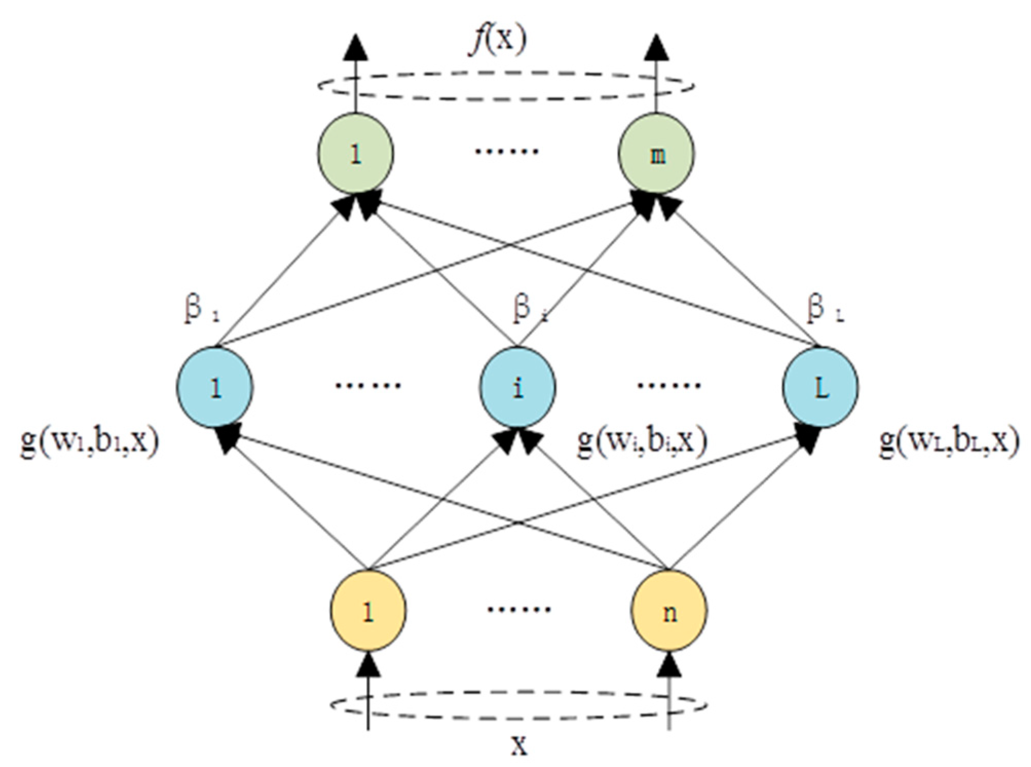
A number of training models have immense challenges for training. Contrary to traditional neural networks, the ELM theory proves that, for the majority of neural networks and learning algorithms (for instance, hidden layer activation as function Fourier series, and biological learning), hidden layer nodes or neurons do not require iterative adjustment. Additionally, they can randomly initialize the input weight and bias; for instance, the ELM network model (Figure 1).

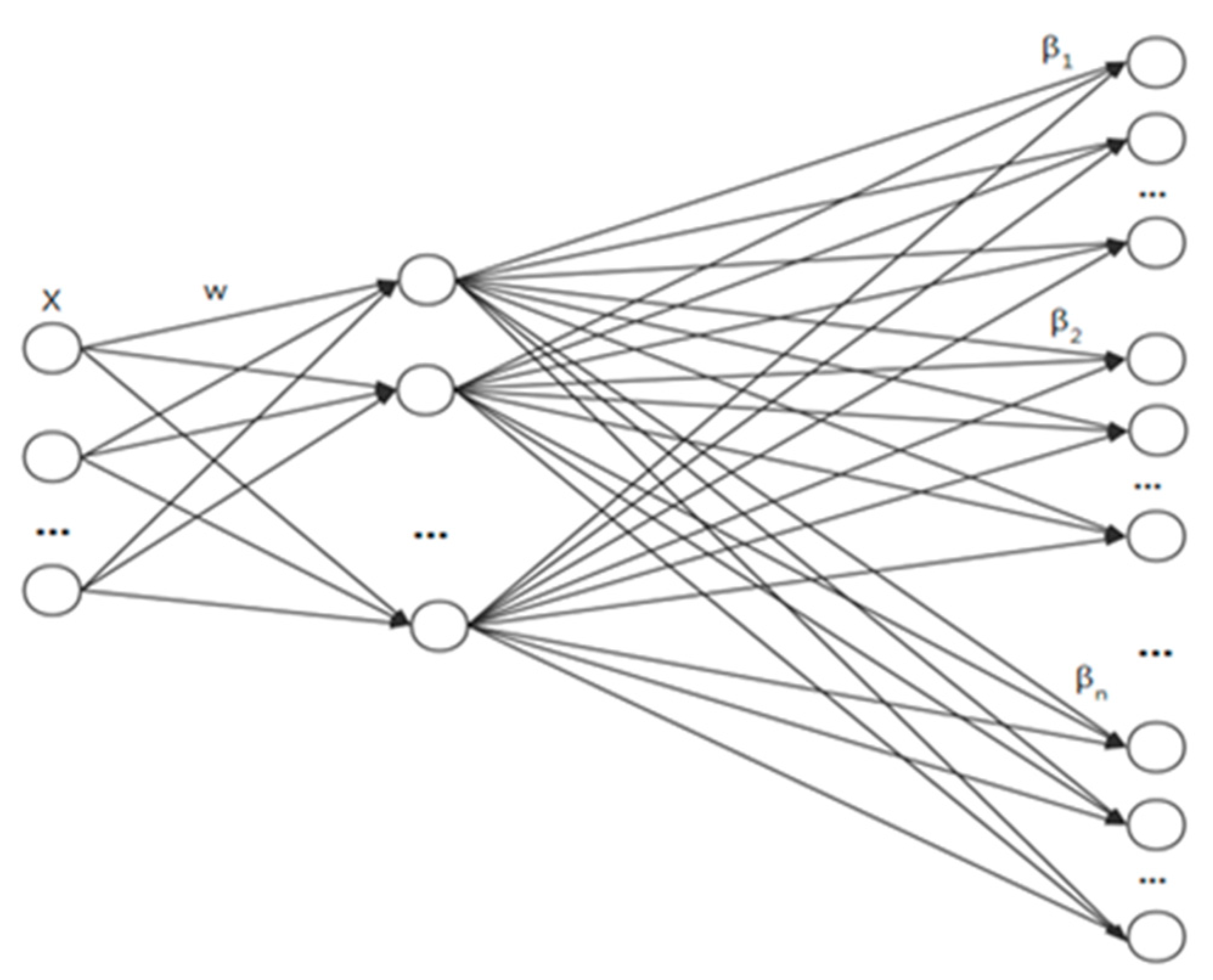
The weights between the hidden nodes and the input of the ELM are randomized. In practical applications, multiple ELM models are capable of sharing the same random input weight. Figure 2 demonstrates that multiple submodels share a similar structure. This indicates that the number of input nodes, the number of hidden layer nodes, and the number of output nodes are all the same. In the meantime, the ELM algorithm requires the randomization of the input layer weights and the network structure between the input X, wherein the hidden layer can be shared.

A complex ELM network can be transformed into a S-ELM-Cluster structure, dividing the tasks and improving the processing speed. This transformation also has the potential to divide the input sample into a number of blocks. The different inputs enter the different ELM submodels to train, while not impacting each other, which is suitable for parallel processing. In the use of the multimodel training method, the model itself can express a lot of information that has the ability to lower the workload of feature processing. In the meantime, the S-ELM-Cluster proposed here is capable of turning multiple features into multiple models.

Features are the inputs of machine learning that can be classified into two types, in accordance with to the diversified features of the data: Affiliated features and phenomenon features. Affiliated features can be enumerated and utilized for subdataset partitioning. In the meantime, the phenomenal features are employed for training models on subdatasets. With the subset, the training algorithm is trained as per the distribution of the data in the feature space, aimed at attaining the recognizer.

The enumeration partitioning methodology itemized all of the possible combinations of subsidiary features with the use of an enumeration form, in order to realize each combination. Nevertheless, in practice, feature input is intricate and diverse, owing to the fact that it is likely to include both numerical and enumerative features. Numerical characteristics such as the congestion value are comparatively larger. They describe the level of a specific nature. Nonetheless, enumerated features such as the road grade do not have a relative size relationship between different values. Instead, they only describe the category of a specific nature. Continuous numerical features are unable to directly enumerate each value. Accordingly, it is quite essential to discretize the numerical features and generalize them into multiple intervals. If the value range of the congestion value feature is (0,100), it can be segregated into 10 segments following the discretization, (0,10), (1,20), …, [90,100]. Further, numerical features are discretized into enumerative features.

The selected subsidiary feature group a consists of p enumerated features; that is, $a=\left(a_1,a_1, \dots ,a_p\right)$, where the arbitrary feature $a_i$ can have different values of $q_i$. Eventually, the enumerable classes of a are theoretically ${{\displaystyle \prod }}_{i=1}^p{q}_i$. In this manner, the samples can be accurately segregated into ${{\displaystyle \prod }}_{i=1}^p{q}_i$ subsets in the subsidiary feature space. Each sample is capable of entering a subset of data based on the enumerated value. Subsequent to that, the same data subset can be unified and trained in accordance with the phenomenal features.

If the feature group $a=\left(a_1,a_1, \dots ,a_p\right),$ it is selected as the subsidiary feature. The other feature groups d form the phenomenal feature. $D^{a+d}$ is a single model over-bound learning machine classifier with the highest average accuracy in the global feature space, composed of the subsidiary feature group a and the phenomenal feature group d. After subdividing into K independent subspaces according to subsidiary feature a, the global correct classification probability of a single model classifier can be expressed as follows:

$$P\left(D^{a+d}|R_n\right)={\displaystyle \sum }_{j=1}^{K}P\left(D^{a+d}|R_j\right)P\left(R_j\right)$$

(12)

where $P\left(R_j\right)$ is the probability that a sample is partitioned into $R_j$ subspace, and $R_n$ is the global space. In addition, $P\left(D^{a+d}|R_j\right)$ is the probability that the samples in $R_j$ will be correctly divided by the classifier $D^{a+d}$.

Since the values of affiliated features are the same in each independent subspace, the information content of the affiliated data is 0. The affiliated feature a has no influence on the classification results of this subset. Thus, the classification of $D^{a+d}$ on $R_j$ can be regarded as a classifier with the same network parameters, trained after the affiliated features are proposed in $R_j$ space:

$$P\left(D^{a+d}|R_j\right)=P\left(D^d|R_j\right)$$

(13)

The over-limited learning machine can obtain the global optimal solution on the subset based on phenomenal data training in the subset of the data set, by optimizing the parameters. As such, the recognizer $D_j^d$, with the highest recognition accuracy in $R_j$, can be obtained using the following equation:

$$P\left(D_j^d|R_j\right)\ge P\left(D^d|R_j\right)$$

(14)

By synthesizing all the recognizers in the subspace, the recognition accuracy of $D^{*}$ in the over-limited learning cluster system can be expressed as follows:

$$P\left(D^{*}|R_n\right)={{\displaystyle \sum }}_{j=1}^{K}P\left(D_j^d|R_j\right)P\left(R_j\right)\ge {{\displaystyle \sum }}_{j=1}^{K}P\left(D^{a+d}|R_j\right)P\left(R_j\right)=P\left(D^{a+d}|R_n\right).$$

(15)

From Formula (15), the over-limited learning cluster will be better than a single global optimal classifier. Based on this theory, and due to the high similarity of data in the subspace, the affiliated features can be eliminated in training.

The fast learning algorithm of the whole S-ELM-Cluster is as follows (Algorithm 1):

Algorithm 1. S-ELM-Cluster fast learning

Train  Input: Training sample X, sample marker T, number of hidden layer neurons L, regularization coefficient C, excitation function $\tilde{g}\left(x\right)$.  Output: All enumerated types $\left\{v_1,v_2, \dots ,v_K\right\}$, hidden layer output weights group $\beta =\left\{{\beta }_1,{\beta }_2, \dots ,{\beta }_K\right\}$, shared hidden layer network $\tilde{h}\left(x\right)$. 1. Start 2. Randomly generate input weight w and hidden layer offset b to form a shared network $\tilde{h}\left(x\right)$. 3. Extract some enumerated features and numerical features of training data a as enumerated feature group, and the rest feature group d is phenomenal feature group. 4. Divide the training data X into $\left[X^{\left(a\right)},X^{\left(d\right)}\right]$ to obtain all the enumeration types $\left\{v_1,v_2, \dots ,v_K\right\}$ of $X^{\left(a\right)}$. 5. According to each enumeration type, $X^{\left(d\right)}$ is divided into K data subset $\left\{X_1^{\left(d\right)},X_2^{\left(d\right)}, \dots ,X_K^{\left(d\right)}\right\}$. 6. For i = 1 to K 7. Calculate the output matrix ${\tilde{H}}_i=\tilde{h}\left(X_i^{\left(d\right)}\right)$ of the hidden layer on the subset $X_i^{\left(d\right)}$. 8. Calculate hidden layer weight ${\beta }_i$ by Formula (7) or (8). 9. End for 10. End Test Input: Samples to be tested $x_{new}$ Output: Testing sample mark $y_{new}$ 1. Start 2. Divide the samples to be tested into $\left[x_{\mathrm{new}}^{\left(a\right)},x_{\mathrm{new}}^{\left(d\right)}\right]$, and $v_{*}=x_{\mathrm{new}}^{\left(a\right)}$ is matched in all enumeration types $\left\{v_1,v_2, \dots ,v_K\right\}.$ 3. Mark the sample to be tested $x_{\mathrm{new}}$ is $y_{\mathrm{new}}=\tilde{h}\left(x_{\mathrm{new}}\right){\beta }_{*}$ 4. End

3. Short-Term Congestion Prediction Based on the Symmetric Extreme Learning Machine Cluster Algorithm

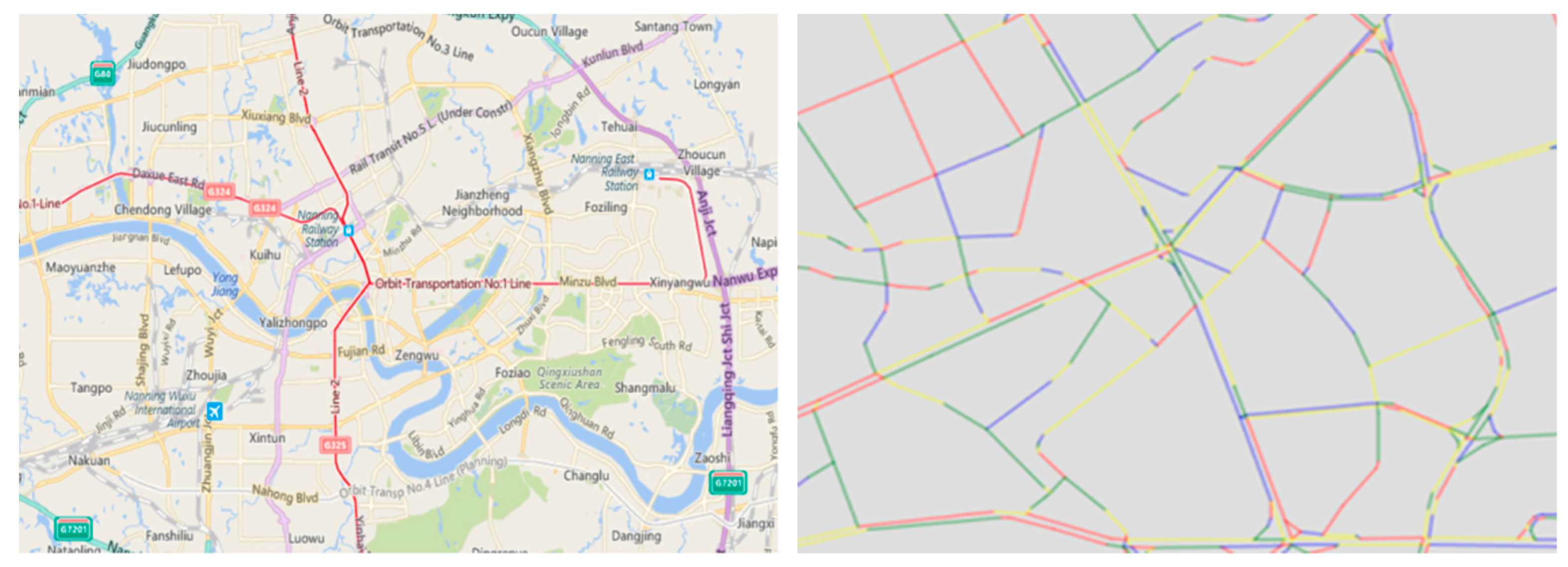
To facilitate handling, the whole road network is divided into many segments based on the topology of the road connections. These segments are hereinafter referred to as the road sections (Figure 3). A road section is the basic unit of evaluation and prediction.

The S-ELM-Cluster algorithm is used to generate a submodel for each section. These submodels have the same network structure. Additionally, these multiple submodels can share one input layer node to form the S-ELM-Cluster. As a node of the whole model, each submodel only realizes the prediction of a particular section, and the function is limited. All of the submodels form a huge complex network capable of predicting the whole network. In this paper, a total of 18,328 sections needed to be predicted. Therefore, the number of S-ELM-Cluster submodels is 18,328.

3.1. Time Series Analysis of Traffic Flow

A time series is an array of data points indexed (or listed or graphed) in time order. Usually, a time series is termed as a sequence taken at successive equally spaced points in time. The time series analysis is a quantitative application of mathematical statistics employed for the purpose of analyzing historical data in the past, in addition to predicting the development trend of things in the future. It is an extensively employed analysis. Any scenario which can generate time series data can make use of time series features for the analysis of trends. Examples include time series based on the wind speed prediction, time series based on human flow prediction, and time series based on tidal prediction. In general, time series prediction is a reflection of three kinds of actual change laws, which include trend change, periodic change, and random change.

From this perspective, the time series of traffic congestion index can be generated by changing the traffic congestion index over time. It suggests that, if the congestion value is set at $C_{t_i}$ and at the time $t_i$, the following sequence can be generated over time:

$$C_{t_1}, C_{t_2},C_{t_3}, C_{t_4},C_{t_5}, C_{t_6}, \dots , C_{t_i} ,\dots$$

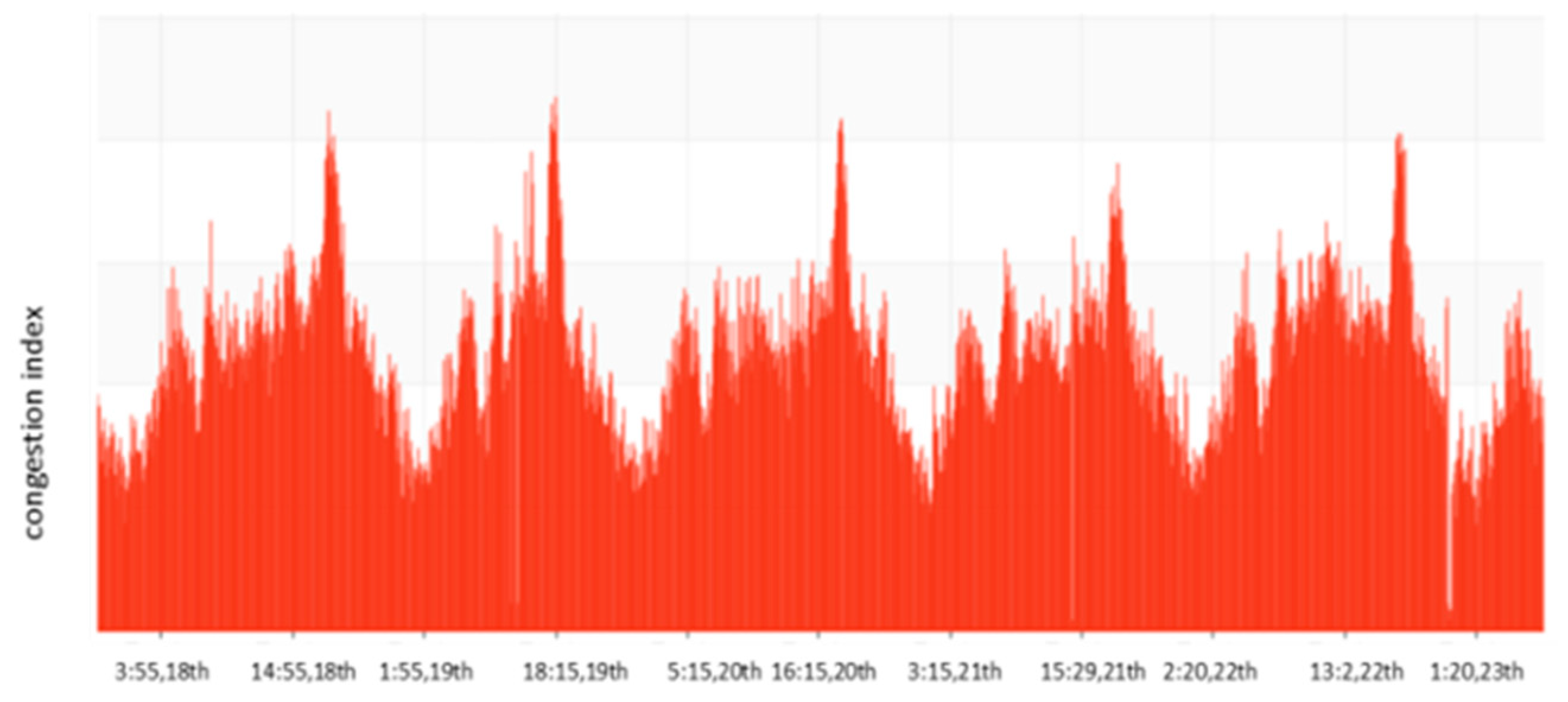
Together with this, the time series of the traffic congestion index has a robust self-similarity in a specific period. Actual statistics shed light on the fact that, even though the traffic flow curve of the same section fluctuates, there are also the features of periodic changes. In a longer statistical cycle, for instance, a day or a week, a clear periodicity can be figured out. Figure 4 illustrates the change of the congestion index of a section of Xiangzhu Avenue in Nanning City between 18 and 22 January 2017. The horizontal axis indicates the time, whereas the vertical axis represents the congestion index.

As is evident from the graph, the observation period of the sky level indicates that the section is expected to reach an early peak at 8 o’clock in the morning, and a late peak at 6 o’clock in the evening, every day. There also exists a robust self-similarity between the day and the week. To an extent, this self-similarity is the inherent law of traffic change. Conversely, considering a longer statistical cycle, it is also in line with the people’s travel demands, which shows coincidence with Nanning’s urban travel rate as well.

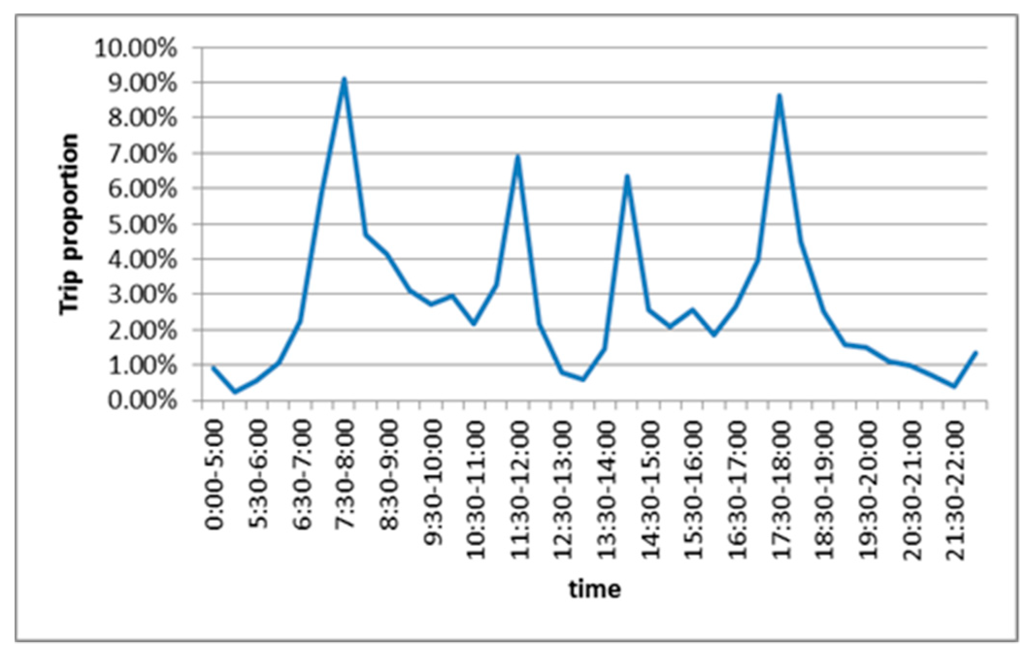
Considering the time distribution of the residents’ all-way travel, residents’ travel has a significant feature of an early peak and late peak. For instance, the early peak occurs from 7:00 to 8:00, wherein the travel volume is concentrated, which accounts for 17.96% of the total day travel volume. The late peak takes place from 17:00 to 18:00, which accounts for 13.91% of the total day travel volume. Besides that, there are two small peaks before and after lunch, resulting from residents going out or returning home for the purpose of dinner and rest. Figure 5 demonstrates that the proportion of traffic trips is symmetrical in time. Such a travel demand is comparatively more stable, as well as having a robust correlation with the results of Figure 4. In addition to this, the travel time demand confirms that the regularity of the change of the traffic congestion value is stable, and that the traffic congestion index has a specific stability, confirming the suitability of the use of the time series analysis methodology for the prediction of traffic.

However, with a shortening observation time scale, the traffic system gradually changes from a deterministic state, to a nonlinear state, to a chaotic state, and finally to a random state. This suggests that the prediction time interval should not be extremely short. Subjected to this condition, the current paper aims at predicting the minute-level, or once a minute, prediction of traffic. As evident from the above analysis, the present paper finds that the change of the traffic congestion index is a typical time series, with a specific level of continuity and periodicity. The traffic congestion data also reveals significant randomness and uncertainty. The neural network is able to identify intricate nonlinear systems. In this manner, it is more suitable for short-term traffic congestion index prediction.

3.2. Traffic Congestion Index

The specific definition of traffic congestion has no unified standard. The purpose of traffic congestion evaluation is to propose a calculation index and quantify the current road congestion. In China, Nanning is one of the urban centers that has established a complete road traffic monitoring system. Through long-term investigation and understanding of the characteristics of roads in Nanning, this paper proposes the traffic congestion evaluation index, which is in the range of [0,100]. This paper finds that when the speed is 0, the road is extremely congested; that is, the congestion value is 100. When the speed is infinitely close to infinity, this means that the road is close to an unlimited flow; that is, the value of road congestion is 0. According to the citizens’ travel habits and the urban road traffic operation evaluation index system of Nanning, traffic congestion can be divided into five levels (

Table 1. Different road congestion levels according to average speed and congestion standard.

		Unblocked	Basic Unblocked	Mild Congestion	Moderate Congestion	Serious Congestion
Speed interval (km/h)	Highways, expressways	(65,∞)	(50,65]	(35,50]	(20,35]	[0,20]
	Main road	(40,∞)	(30,40]	(20,30]	(15,20]	[0,15]
	Secondary roads, branches	(35,∞)	(25,35]	(15,25]	(10,15]	[0,10]
Congestion value		(0,20)	[20,40)	[40,60)	[60,80)	[80,100]
Map show color		Light green	Green	Yellow	Red	Deep red

).

The relationship between the traffic congestion index $C\left(x\right)$ and vehicle speed $x\left(x\ge 0\right)$ can be expressed as:

$$C\left(x\right)=100 - \left(\frac{1}{1 +{ \mathrm{e}}^{-\partial x}} - \frac{1}{2}\right)·200$$

(16)

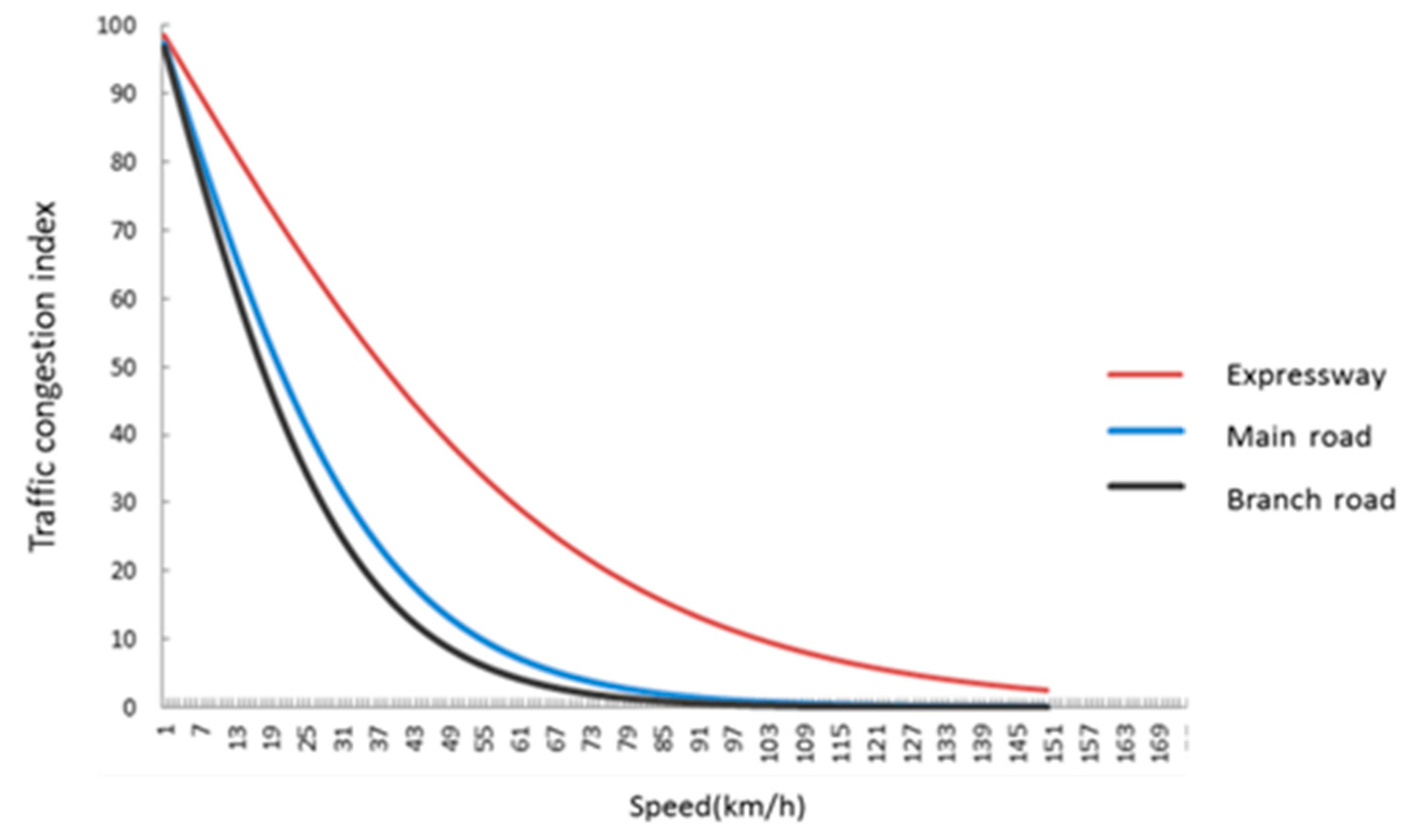
In Formula (16), the parameter $\partial$ is different with diverse road levels. Highways, expressways, main roads, secondary roads, branches, and other road grades at the same speed experience traffic congestion in different ways. However, when the speed is the same, then it means that the road level will be higher, and the congestion index will be bigger. Parameter $\partial$ is used to reflect the impact of road grades on the traffic congestion index.

According to the fitting of the actual data,

Table 2. Values of parameter ∂ with different road levels.

Highways, Expressways	Main Roads	Secondary Roads, Branches
0.028	0.052	0.065

summarizes some different specific parameters.

Figure 6 illustrates that the higher the road equivalence, the greater the congestion index at the same speed.

At present, there are more than 8000 floating cars in Nanning, loaded with GPS vehicles, which regularly report the speed, angle and other information to the command center, and cover 70% of the roads in Nanning every five minutes. According to the real-time traffic report of the floating cars, a number of complex algorithms are employed to match the floating vehicles to the surrounding roads. It is also possible to calculate the average speed of the road and the road congestion index.

This paper aims to predict the traffic congestion index in the next 0–30 min by using the S-ELM-Cluster. Nanning’s daily accumulated monitoring data, traffic congestion index evaluation, road network, municipal, and other information provide a solid data support for the prediction of the traffic congestion index.

3.3. Feature Extraction and Modelling

3.3.1. Section Clustering

The administrative area where the road is located is partly referred to in the environmental information of the road. For example, the road in the commercial area is poor in the evening, and the traffic in the office building is heavy. The road condition is also poor. As expected, the administrative area where the road is located is strongly related to the congestion of roads. In practical applications, the administrative area of the road is difficult to obtain automatically, since the area is changed. The feature extraction module cannot be updated automatically. This paper uses the following clusters to replace the administrative region characteristics:

$C_{i,j} \left(0\le x_{i,j}<100\right)$, which is the congestion value of road i at time j. For a definite road i, ${[C_{i,0}, C_{i,1}, C_{i,2},\dots ,C_{i,190}]}^T$ is the congested value vector of the road in one day. At the same time, the congestion value matrix of all roads is expressed as follows:

$$\begin{array}{c}{C}_0={[C_{0,0},C_{0,1},C_{0,2},\dots ,C_{0,190}]}^T\\ C_1={[C_{1,0},C_{1,1},C_{1,2},\dots ,C_{1,190}]}^T\\ \dots \\ C_n={[C_{n,0},C_{n,1},C_{n,2},\dots ,C_{n,190}]}^T\end{array}.$$

(17)

A line of the congestion matrix describes the change of the road congestion value in a day, and the time series value of the congestion value as a feature. To an extent, it describes the change law of traffic flow in each section. Using the k-means unsupervised clustering method, the road is clustered into k clusters. At the same time, the road congestion value of similar clusters is related. The variation of the congestion value of the sections of different clusters is quite different. Clusters logically represent the regional characteristics of road sections. In this paper, k = 50 divides Nanning City’s roads into 50 logical regions.

3.3.2. Feature Extraction

A number of factors exert an impact on the traffic congestion index. These factors can be divided into three distinct categories:

• Road factors: These include the road level, lane number, road traffic light distribution, road intersection distribution, and road related inherent features.
• Environmental factors: These include the urban functional areas on which roads are located, and whether there are schools, large public places or other factors that affect the traffic flow.
• Sudden factors: These include uncertain factors such as weather changes, traffic accidents, traffic control, and other key activities.

Road factors and environmental factors are comparatively more stable factors. They make the traffic congestion index have robust periodicity and self-similarity in the medium- and long-term. Nonetheless, sudden factors like the environment, weather, accidents and people are likely to make traffic congestion uncertain. With regards to the traffic congestion prediction, the use of the appropriate model feature is the most significant factor impacting the accuracy of prediction.

Nowadays, the urban road network in Nanning City is divided into 18,328 sections (Figure 3). Accordingly, the road segment constitutes the basic unit of prediction. There are also lots of factors impacting the traffic. Some of these factors are relatively fixed, even though they change at times. In that case, there are numerous factors requiring consideration in prospective selection. A real-time traffic prediction system requires the feature to be acquired and updated automatically. By means of a series of experiments and feature selection, the following features were selected as input features in the current paper:

• Road clusters, discrete features, 1, 2, 3, 4, …, 50, a total of 50 kinds of values.
• The current time, discrete characteristics, 06:05, 06:15, 21:55, a total of 191 values.
• The congestion values in the past eight historical periods: A continuous feature with a range of 0–100, wherein each historical period is ten minutes.
• Road level: Highways, expressways, main roads, secondary roads and branches.
• The number of adjacent roads at the road entrance: This continuous feature is 0, 1, 2, 3.
• The number of adjacent road connections at the road section: Continuous characteristics, with a value of 0, 1, 2, 3, ….

In practical applications, the feature input is both intricate and varied, likely including both numerical and enumerated features. The range, type, and dimensions of feature values are different, accordingly being unable to be investigated directly. That is why it is deemed essential to preprocess and standardize the features. In general, numerical features should be discretized into multiple intervals. The numerical and enumerative features should also be unified as enumerative features.

Enumerated features constitute an array of tags requiring further two-valued processing to be sent to the model. The so-called two-value feature is primarily the 0/1 feature. This feature takes only two values: 0 or 1. The method of converting enumeration values to two-value features deals with mapping enumerated features into multiple features. Each of the features corresponds to a specific enumeration value. For the purpose of distinction, the following enumeration features are referred to as cluster features; on the other hand, the number of two-valued features transformed from enumerated features are considered single features.

Overall, variables either suggest measurements on some continuous scales, such as the traffic congestion index of the last time in this case or represent information regarding some categorical or discrete features, such as the current time in the above features. The features put to use in this paper mix categorical features with real-valued features and should be transformed into all categorical or real-valued features. In our case, all of the categorical features are subdivided into a number of single real-valued features, with the value set as either 1 or 0. For instance, the feature current time will be transformed into 192 new features. Each of them is 0 or 1 in order to indicate if it appears or not. Accordingly, all of the features become real-valued and can be equally evaluated as well. In accordance with the experiments in practice, such a transformation increases the accuracy rate by 2.2% in comparison with the direct use of the original feature.

4. Implementation and Experimental Results

4.1. Data

The applied research in this paper is based on the traffic in the main urban area of Nanning City. The floating vehicle data used is the real-time data collected by the Traffic Management Department of Nanning City. In addition, the electronic map data of Nanning City is also used. The electronic map data is the basic data for matching the track data of the floating vehicle data. The goal of trajectory data matching is to locate it on the actual road in the electronic map and establish an association with it. All analysis and prediction are based on floating vehicle data for the entire experiment. At present, Nanning City has built a complete floating vehicle detection system. The system consists of more than 8000 floating vehicle monitoring points, composed of buses and taxis, which can monitor the traffic conditions in the city at all times. The system obtains real-time floating vehicle data based on the floating vehicle interface provided by the Transportation and Management Department of Nanning City. The data returned by the floating vehicle contains location information (latitude and longitude), as well as information such as speed, angle, and GPS accuracy. It covers almost all the main roads of Nanning.

This section mainly tested the performance of the S-ELM-Cluster model on the basis of time series characteristics on a traffic congestion data set in Nanning and compared the S-ELM-Cluster algorithm with the ELM algorithm, along with other popular machine learning algorithms like Logistic Regression (LR), Support Vector Machine (SVM), and gradient boosting decision tree (GBDT). Other than the special instructions, all the experiments were run on the Ubuntu 12.04 machine. The physical memory of the experimental machine was 32 GB, and the processor was Duo i7 2.50 GHz. The symmetric-ELM-cluster was implemented in Python and run in a Python 2.7 environment.

Traffic congestion data in Nanning City were divided into three categories, which included working days, weekends, and major festivals. Three data sets were formed based on the feature extraction differences. Taking the accumulated data of five main days (6:00–24:00) as the training data, a comparative experiment using all road data revealed that the cluster learning method has a better learning effect in large-scale traffic forecasting.

Table 3. Training and test data of the congestion prediction experiment based on the symmetric extreme learning machine cluster (S-ELM-Cluster).

Training Data Set	Training Sample Source	Number of Training Samples	Test Sample Source	Number of Test Samples
Working day	20–24 March 2017	4,961,698	27 March 2017	1,036,785
Weekend	Saturdays and Sundays, March 2017	5,023,698	26 March 2017	968,254
Major festival	Ching Ming Festival and May Day in 2017	5,069,547	2 May 2017	1,187,234

summarizes the experimental data.

In the experiment, the prediction results of the test samples were compared with the actual congestion values. The regression results are continuous integers varying between 0 and 100. In this paper, prediction is correct when $|y_{\mathrm{truth}}-y_{\mathrm{estimate}}|\le 25$; $y_{\mathrm{truth}}(0\le y_{\mathrm{truth}}<100)$ is the actual congestion index in the testing data while $y_{\mathrm{estimate}}(0\le y_{\mathrm{estimate}}<100)$ is the estimate result predicted by the models. The results confirm that when the actual congestion values are within the congestion level of the prediction results, then the prediction results would be considered accurate. Otherwise, the prediction is inaccurate. Also, the accuracy of the congestion prediction model could be counted.

4.2. S-ELM-Cluster Model Tuning Test

The S-ELM-Cluster forecasting model, based on time series, should optimize three parameters:

4.2.1. The Length of Time Series

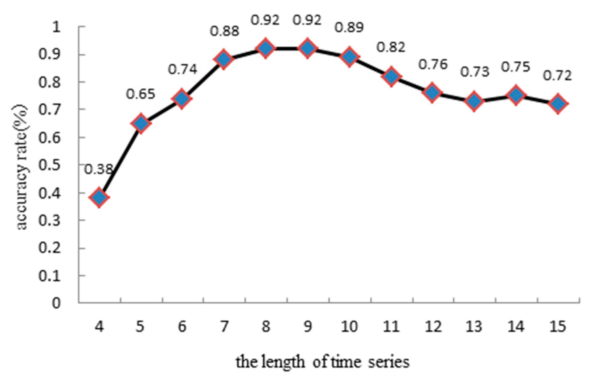
The system creates assessment output every 10 min so as to portray the present urban traffic situation for every road segment. These data gradually become historical. The length of time series cannot be given by experience before training. For time series modeling, the length of the time series is usually determined by using the sample autocorrelation function (ACF) [24,25] and the sample partial autocorrelation function (PACF) [24,25]. The ACF and PACF are commonly used model identification tools and are usually used to provide the initial guess of sequence length. In order to further determine the optimal model order, other tools need to be used. The most commonly used criteria are the Akaike information criterion (AIC) [26] and Bayesian information criterion (BIC) [27], based on information theory. Through reading relevant literature, this paper found that many scholars selected traffic historical data series lengths of 8 or 9. In this experiment shown in Figure 7, the length of the time series is found to increase from four to observe the prediction accuracy of the test set.

From the results, we find that when the time series is too short, the sequence will have less information, and will be more random. However, the prediction accuracy of the model is lower. In contrast, when the length of the time series increases gradually, the prediction accuracy also increases steadily. However, when the sequence length is equal to 8, the maximum value is reached, and stability is subsequently maintained. Additionally, when the length of the time series is greater than 10, the prediction accuracy begins to significantly decrease. Thus, we notice that a time series length of 8 is better and can obtain the highest accuracy.

4.2.2. The Regularization Coefficient C and the Number of Hidden Layer Nodes L

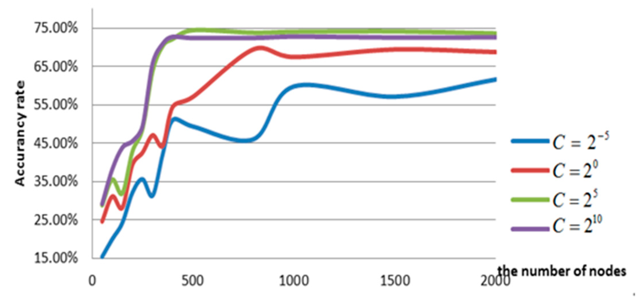
Based on the theory, the training effect of the ELM is affected by the regularization coefficient C and the number of hidden layer nodes L, which is more sensitive to the regularization coefficient C. At the same time, L is less disturbing to the model when its value is larger, and the performance of the ELM is more stable. Figure 8 shows the effect of these two parameters on the overall S-ELM-Cluster network performance in the Nanning datasets.

As illustrated in Figure 8, the regularization coefficient and the number of hidden layer nodes have an effect on the S-ELM-Cluster. Although the regularization coefficient is large, the accuracy of the S-ELM-Cluster is relatively high, if not necessarily optimal.

The influence of the number of hidden layer nodes was found to be relatively regular. Under the values of different regularization coefficients, the number of hidden layer nodes was revealed to be relatively small as well, and the S-ELM-Cluster accuracy had a large amplitude fluctuation. However, when the number of hidden layer nodes was larger, the accuracy was stable and at a high level.

4.3. Comparison Test of the S-ELM-Cluster and ELM

In this section, the single ELM is compared with the S-ELM-Cluster model. The number of hidden layer nodes of the ELM was found to be 1000. All experiments were performed through cross validation. In addition, all the training sets were randomly divided into four smaller subsets, taking three of them at each time as training sets and the other as a test set.

From the experimental results, the S-ELM-Cluster algorithm was found to be more accurate—almost 1.5 times more than the ELM algorithm. However, a single model could not learn the rules correctly, and the model obtained by training had no practical value. To improve the prediction accuracy with a single model, it is necessary to artificially depend on the test to excavate other features, and timing features as input features, for training. Still, it would inevitably lead to an increase in the dimension of the feature, which may result in the curse of dimensionality and an increase in training time.

After using the S-ELM-Cluster algorithm, many small samples were sent to different ELM models. The number of input samples was less, and the complexity of a single ELM was reduced.

Table 4. Comparison between the ELM and S-ELM-Cluster.

Algorithm	Training Time (s)	Accuracy
ELM	116	64.28%
S-ELM	67	65.77%
S-ELM-Cluster (single process)	134	92.99%
S-ELM-Cluster (20 processes)	9.2	93.12%
S-ELM-Cluster (40 processes)	5.1	93.04%

shows that the training time of the single process S-ELM-Cluster and ELM is not different, although the accuracy rate is 1.5 times that of the latter. From the table, it is also evident that the S-ELM-Cluster training time of 20 processes is 12 times faster than that of a single ELM on the experimental data set. The S-ELM-Cluster of 40 processes was revealed to be 23 times faster than that of a single ELM.

From the experimental data of this section, we realized that in some cases, the use of the multimodel S-ELM-Cluster was faster than a single model (easy to parallelize), and had better generalization ability.

4.4. Comparison of the S-ELM-Cluster and Other Algorithms

Although there are many types of learning algorithms that are widely used in traffic forecasting, this paper compares the S-ELM-Cluster algorithm with other types of machine learning algorithms on the traffic congestion prediction training data set. The comparison of algorithms used in this paper include logical regression (logistic regression), ridge regression (ridge regression), and GBDT regression (gradient boosting decision tree regression). These algorithms are implemented in the Python Sklearn 1.4 machine learning library, where the depth of GBDT is 9, LR introduces L1 regularization, and the other parameters are kept at default.

Table 5. Comparisons of different learning algorithms. GBDT: Gradient boosting decision tree. LR: Logistic Regression.

Algorithm	Training Time (s)	Accuracy
S-ELM-Cluster (40 processes)	24.63	92.08%
GBDT	4501.16	92.10%
Ridge	893.23	89.49%
Lasso	9.34	86.79%
LR	7.69	74.15%

summarizes the results of the experiment.

From Table 5, it can be seen that the accuracy of the S-ELM-Cluster and GBDT is high, reaching about 90%. From the training time, the S-ELM-Cluster benefits after the parallel optimization is clear. Compared with the GBDT and Ridge algorithms, the S-ELM-Cluster can reduce the hour-level training task to the minute-level, with only 1/3 min required for completion. The Lasso and LR algorithms are the most commonly used linear models due to their fast computing speed. As such, these linear models have been widely used in large data, including statistical analysis, computing advertising, and search sorting. Unfortunately, while the training speed of the data set is extremely fast, the prediction accuracy is extremely different from other algorithms.

Experiments with linear SVM were carried out on the same data set. However, the experiment lasted too long. Even after 35 h, no result had been obtained. To facilitate comparison, experiments were conducted on the sub-data set, while retaining the training and testing samples of the 1/10 road segment (

Table 6. Comparison between the S-ELM-Cluster and SVM: Support Vector Machine

Algorithm	Training Time (s)	Accuracy
S-ELM-Cluster (single process)	10.57	90.91%
SVM	686.85	87.87%

).

The results indicate that the S-ELM-Cluster is more accurate than SVM. It also confirms that the S-ELM-Cluster under a single process is more than sixty times faster in terms of training speed than SVM. Considering the two aspects of accuracy and efficiency, the S-ELM-Cluster is more suitable for mass traffic congestion data sets than SVM.

4.5. Prediction Results Evaluation

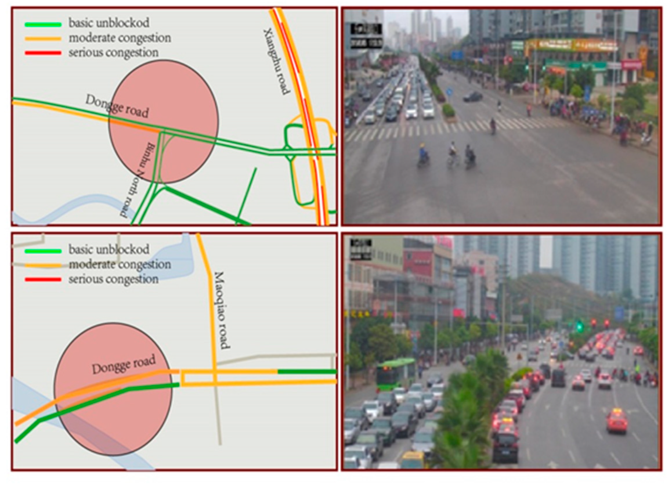
The accuracy of the prediction is a quantitative analysis of the need to combine the actual situation to examine whether the prediction results correspond with the actual situation, and whether it is consistent with the intuitive feelings of the citizens. Therefore, this paper combines the prediction results with video surveillance in Nanning City, and qualitatively evaluates the prediction results. The assessment outcomes satisfy the true condition, as illustrated in Figure 9. In the map, green represents basic unblocked traffic, orange shows moderate congestion, and red means serious congestion. Seen from the image taken by surveillance cameras, the traffic evaluation accurately reflects the road traffic congestion at that time.

Figure 9 shows a comparison of the 10-min forecast results between the prediction system and the real congestion situation at 15:50 on 5 March 2017. In Figure 9, the upper left image is the 10-min visual result of the intersection between Dongge Road and Binhu North Road. Similarly, the upper right image exhibits the true intersection 10 min later. From the west to the east, the results of the predicted results are yellow, while the other directions are unblocked. The corresponding pretest results are green. Notably, the predicted results are consistent with the real road conditions. The lower right image shows the real road conditions of the intersection of Dongge Road and Maoqiao Road. Meanwhile, the left western lane and the right east lane are slow and congested, which is also consistent with the prediction from 10 min earlier.

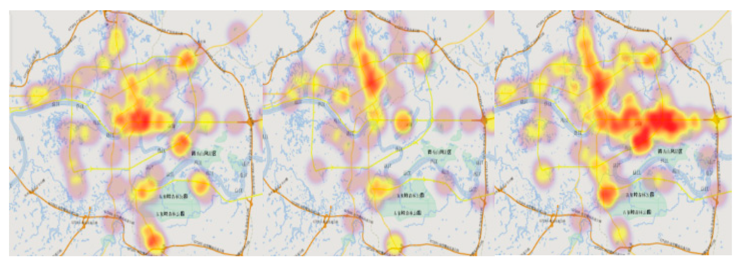
Figure 10 is the visual result of a cluster within the 10-min forecasts carried out on 5 March 2017. The 10-min forecast at 8:00, 11:00, and 18:00, respectively, can be seen from left to right. From the geographical spatial clustering analysis, it is also clear that traffic congestion in Nanning City is mainly concentrated in the central railway station, Chaoyang business circle, expressway out of the city area, and the construction area of the track and interchange. More specifically, the Chaoyang business circle and railway station are the main distribution points of urban traffic flow. They are also affected by the poor traffic conditions of the old urban road network, and the construction of the rail stations. These two areas are the most affected by urban traffic congestion, with all days being relatively congested. This observation is consistent with the actual situation in Nanning City.

5. Conclusions

In this paper, inspired by the theory of ELM and multimodels, a novel extreme learning machine cluster algorithm was proposed. The S-ELM-Cluster has several ELM submodels, each of which is only responsible for learning a particular class of samples. Each cluster of samples can achieve the global optimum and obtain a higher prediction accuracy. The ELM submodels are independent of each other, easy to parallelize, and suitable for large-scale computations. Drawing from the experimental results, the prediction method based on the S-ELM-Cluster has high accuracy in short-term predictions. Additionally, the prediction results were found to be in line with the actual situation. They were also highly reliable. Therefore, traffic congestion prediction based on the S-ELM-Cluster has a strong practical value. In future, it is necessary to carry out experiments on a public dataset to further verify the effectiveness of the algorithm.

References

- Ghosh, B.; Basu, B.; O’Mahony, M. Bayesian Time-Series Model for Short-Term Traffic Flow Forecasting. J. Transp. Eng. 2007, 133, 180–189. [Google Scholar] [CrossRef]
- Guo, J.; Huang, W.; Williams, B.M. Adaptive Kalman filter approach for stochastic short-term traffic flow rate prediction and uncertainty quantification. Transp. Res. Part C 2014, 43, 50–64. [Google Scholar] [CrossRef]
- Yu, G.; Zhang, C. Switching ARIMA model based forecasting for traffic flow. In Proceedings of the International Conference on Acoustics, Speech, and Signal Processing, Brighton, UK, 12–17 May 2004; Volume 2, pp. 429–432. [Google Scholar]
- Zhang, Y.; Ye, Z. Short-Term Traffic Flow Forecasting Using Fuzzy Logic System Methods. J. Intell. Transp. Syst. 2008, 12, 102–112. [Google Scholar] [CrossRef]
- Xue, J.; Shi, Z. Short-Time Traffic Flow Prediction Based on Chaos Time Series Theory. J. Transp. Syst. Eng. Inf. Technol. 2008, 8, 68–72. [Google Scholar] [CrossRef]
- Cetin, M.; Comert, G. Short-Term Traffic Flow Prediction with Regime Switching Models. J. Transp. Res. Board 2006, 1965, 23–31. [Google Scholar] [CrossRef]
- Abdulhai, B.; Porwal, H.; Recker, W. Short-Term Traffic Flow Prediction Using Neuro-Genetic Algorithms. ITS J. Intell. Transp. Syst. 2002, 7, 3–41. [Google Scholar] [CrossRef]
- Smith, B.L.; Demetsky, M.J. Short-Term Traffic Flow Prediction: Neural Network Approach Transportation Research Record. Transp. Res. Board 1994, 98–104. [Google Scholar]
- Zhao, L.; Wang, F.Y. Short-term traffic flow prediction based on ratio-median lengths of intervals two-factors high-order fuzzy time series. In Proceedings of the Vehicular Electronics and Safety, Beijing, China, 13–15 December 2007; pp. 1–7. [Google Scholar]
- Xu, Q.; Ding, Z. Bi discipline. A real-time prediction method of traffic flow based on dynamic recurrent neural network. J. Huaihai Inst. Technol. Nat. Sci. Edit. 2004, 12, 14–17. [Google Scholar]
- Yang, Q.; Zhang, B.; Gao, P. Based on improved dynamic recurrent neural network for short time prediction of traffic volume. J. Jilin Univ. Eng. Edit. 2012, 4, 887–891. [Google Scholar]
- Jiao, G.T.; Xu, J.; Ma, Y. Traffic volume prediction method based on QPSO-RBF. Traffic Inf. Saf. 2008, 26, 128–131. [Google Scholar]
- Çetiner, B.G.; Sari, M.; Borat, O.A. Neural Network Based Traffic-Flow Prediction Model. Math. Comput. Appl. 2010, 15, 269–278. [Google Scholar] [CrossRef]
- Mussone, L. A review of feedforward neural networks in transportation research. E I Elektrotech. Informationstech. 1999, 116, 360–365. [Google Scholar] [CrossRef]
- Bing, Q.; Gong, B.; Yang, Z.; Shang, Q.; Zhou, X. A short-term traffic flow local prediction method of combined kernel function relevance vector machine. J. Harbin Inst. Technol. 2017, 49, 144–149. [Google Scholar]
- Shang, Q.; Lin, C.; Yang, Z.; Bing, Q.; Zhou, X. Short-term traffic flow prediction model using particle swarm optimization–based combined kernel function-least squares support vector machine combined with chaos theory. Adv. Mech. Eng. 2016, 8, 1–12. [Google Scholar] [CrossRef]
- Huang, G.B.; Zhu, Q.Y.; Siew, C.K. Extreme Learning Machine: Theory and Applications. Neurocomputing 2006, 70, 489–501. [Google Scholar] [CrossRef]
- Aguirre, L.; Lopes, R.; Amaral, G.; Letellier, C. Constraining the topology of neural networks to ensure dynamics with symmetry properties. Phys. Rev. E 2004, 69, 1–11. [Google Scholar] [CrossRef] [PubMed]
- Chen, S.; Wolfgang, A.; Harris, C.; Hanzo, L. Symmetric RBF classifier for nonlinear detection in multiple-antenna-aided systems. Trans. Neural Netw. 2008, 19, 737–745. [Google Scholar] [CrossRef] [PubMed]
- Chen, S.; Hong, X.; Harris, C. Grey-box radial basis function modelling. Neurocomputing 2011, 74, 1564–1571. [Google Scholar] [CrossRef]
- Espinoza, M.; Suykens, J.; Moor, B. Imposing symmetry in least squares support vector machines regression. In Proceedings of the 44th IEEE conference on decision and control, Seville, Spain, 12–15 December 2005; pp. 5716–5721. [Google Scholar]
- McNames, J.; Suykens, J.A.K.; Vandewalle, J. Winning entry of the K. U. Leuven time series prediction competition. Int. J. Bifurc. Chaos 1999, 9, 1485–1500. [Google Scholar] [CrossRef]
- Liu, X.; Li, P.; Gao, C. Symmetric extreme learning machine. Neural Comput. Appl. 2013, 22, 551–558. [Google Scholar] [CrossRef]
- Box, G.E.P.; Jenkins, G.M.; Reinsel, G.C.; Ljung, G.M. Time Series Analysis: Forecasting and Control, 5th Edition. J. Oper. Res. Soc. 2015, 22, 199–201. [Google Scholar]
- Shumway, R.H.; Stoffer, D.S. Time Series Analysis and Its Applications: With R Examples; Springer: Berlin, Germany, 2017. [Google Scholar]
- Akaike, H. A new look at the statistical model identification. IEEE Trans. Autom. Control 1974, 19, 716–723. [Google Scholar] [CrossRef]
- Anděl, J.; Perez, M.G.; Negrao, A.I. Estimating the dimension of a linear model. Kybern.-Praha 1981, 17, 514–525. [Google Scholar]
Figure 1.
The extreme learning machine (ELM) network model.
Figure 2.
Multi-ELMs can share the same random weight .
Figure 3.
The road network is divided into small sections.
Figure 4.
Congestion index of a section of Xiangzhu Avenue between 18 and 22 January 2017.
Figure 5.
Travel demand of Nanning citizens.
Figure 6.
Traffic congestion index of different grade roads.
Figure 7.
Time series length and prediction accuracy.
Figure 8.
The influence of the regularization coefficient (C) and hidden layer node number on the accuracy of the S-ELM-Cluster.
Figure 9.
(left) Ten-minute forecast result in the Dongge Road area and (right) real road condition after 10 min.
Figure 10.
Ten-minute prediction value polymerization analysis at 8:00, 11:00, and 18:00 on 5 March 2017, respectively, from left to right.