Battlefield Target Aggregation Behavior Recognition Model Based on Multi-Scale Feature Fusion

Abstract

In this paper, our goal is to improve the recognition accuracy of battlefield target aggregation behavior while maintaining the low computational cost of spatio-temporal depth neural networks. To this end, we propose a novel 3D-CNN (3D Convolutional Neural Networks) model, which extends the idea of multi-scale feature fusion to the spatio-temporal domain, and enhances the feature extraction ability of the network by combining feature maps of different convolutional layers. In order to reduce the computational complexity of the network, we further improved the multi-fiber network, and finally established an architecture—3D convolution Two-Stream model based on multi-scale feature fusion. Extensive experimental results on the simulation data show that our network significantly boosts the efficiency of existing convolutional neural networks in the aggregation behavior recognition, achieving the most advanced performance on the dataset constructed in this paper.

1. Introduction

Battlefield target aggregation behavior is a common group behavior in the joint operations environment, which is usually a precursor to important operational events such as force adjustment, battle assembly, and sudden attack. To grasp the battlefield initiative, it is important to identify the aggregation behavior of enemy targets. The intelligence video records the different behaviors of the battlefield targets, and effectively identifying the aggregate behavior in the video is the main purpose of this paper.

For the time being, the identification of battlefield aggregation behavior requires a manual interpretation, which is inefficient in battlefield environments. It is an inevi trend for intelligent battlefield development to introduce intelligent recognition algorithms to identify the aggregation behavior. For behavior recognition, intelligent algorithms based on deep learning are the research hotspots. In particular, 3D Convolutional Neural Networks (3D-CNN), which show significant results in behavior recognition, provide a technical basis for battlefield target aggregation behavior recognition.

Unfortunately, the traditional 3D-CNN model has certain drawbacks for the battlefield target aggregation behavior: (1) Compared with the human behavior in the video, the proportion of the target is uncertain in the intelligence video. The existing 3D-CNN network lacks the interaction of multi-scale features. The loss of spatial information in the down-sampling process has a great influence on the detection rate of aggregated behavior; (2) The duration of the aggregation behavior is uncertain, and the down-sampling in the temporal dimension will cause the loss of timing information, which will indirectly affect the final recognition accuracy; (3) Traditional 3D-CNN are computationally expensive. Therefore, the network structure is difficult to flexibly expand, and it is also difficult to cope with large-scale identification tasks.

Our article does not consider the disturbances of complex environmental factors (such as complex weather, etc.), and only focuses on solving aggregation behavior recognition problems with deep learning networks.

We have improved the traditional 3D-CNN. On the one hand, we construct a multi-scale feature fusion 3D-CNN model, which combines multi-scale spatio-temporal data of different convolutional layers to promote the interaction between multi-scale information. This model effectively reduces the information loss caused by the network down-sampling. The model proposed in this paper effectively solves the problem that the size of the battlefield target is different and that the aggregation behavior duration is uncertain, which effectively improves the final recognition accuracy. On the other hand, this paper uses the improved spatio-temporal multi-fiber network as the backbone network, which slices a complex neural network into an ensemble of lightweight networks or fibers. Our network effectively overcomes the huge computational problem of 3D-CNN. At the same time, the depth of the network is deepened, and the nonlinear expression ability of the neural network is increased.

The rest of the paper is organized as follows. In Section 2, related work is discussed. We present our method in Section 3 and the dataset in Section 4. We report the experimental results in Section 5. The conclusion is in Section 6.

2. Related Work

At present, human behavior recognition is a research hotspot in the field of intelligent video analysis. Battlefield target aggregation behavior recognition and human behavior recognition are in the same field of behavior recognition but are not identical. The main reason for this is that single-frame information, which contributes a lot to the human behavior recognition, contributes less to the aggregation behavior recognition. Therefore, multi-frame information must be processed in order to enhance the recognition effect of aggregation behavior. In recent years, researchers have proposed a number of methods for video behavior recognition, which are mainly divided into traditional feature extraction methods [1,2,3] and the method based on deep learning [4,5].

The early traditional methods based themselves on the description of spatio-temporal interest points to extract the features in the video. Wang proposed a dense trajectory method [6], which extracts local features along trajectories guided by an optical flow. This method achieves a state-of-the-art level in the traditional method. However, the extraction process of the traditional underlying features is independent of the specific tasks, and the wrong feature selection will bring great difficulties to the identification. In addition, due to the cumbersome feature calculation, the traditional method is gradually replaced by deep learning.

With the wide application of deep learning in the image field, the video behavior recognition method based on deep learning has gradually become a new hotspot in the field of behavior recognition. The two-stream architecture [7] uses RGB (Red-Green-Blue) frames and optical flows between adjacent frames as two separate inputs of the network, and fuses their output classification scores as the final prediction. Wang [8] constructs a long-term domain structure based on a two-stream architecture. First, multiple video segments are extracted by sparse sampling, and then a two-stream convolution network is established on each segment. Finally, the output results of all the networks are combined for the prediction classification. Many works follow a two-stream architecture and extend this architecture [9,10,11]. RNN (Recursive Neural Network) is excellent in capturing the timing information. Inspired by it, Donahue [12] combines CNN (Convolutional Neural Networks) and RNN to propose a long-term recursive convolutional neural network. More recently, with the increasing computing capability of modern GPUs, 3D-CNN has drawn more and more attention. Varol [13] designed a long-term convolutional network by extending the length of input of the 3D convolutional network, and studied the influence of different inputs on the recognition results. Carreira [14] introduced the two-stream idea into 3D-CNN, innovatively used ImageNet to pre-train 2D-CNN, and then replicated the parameters of the 2D convolution kernel in the time dimension to form a 3D convolution kernel. The recognition accuracy was significantly improved. Although 3D-CNN can learn the motion characteristics from the original frame end-to-end, the network parameters and calculation amount are huge, so the experimental training and testing need to occupy huge resources. Qiu [15] proposed Pseudo-3D (P3D), which decomposes a 3D convolution of 3 × 3 × 3 into a 2D convolution of 1 × 3 × 3, followed by a 1D convolution of 3 × 1 × 1. In addition, S3D [16] and R(2+1)D [17] also applied a similar architecture. Multi-fiber networks [18], which use multi-frame RGB as the input, greatly reduce the computational complexity on the basis of ensuring a recognition accuracy. FPN [19] combines down-top, top-down and lateral connections with using high and low semantic features, which improves the recognition accuracy.

Traditional 3D networks lack the use of multi-scale information, which affects the recognition accuracy of the network. The traditional two-stream model uses 2D-CNN to process images, which is better than the single-stream model but lacks the ability to extract temporal information. In view of the above problems, this paper combines the advantages of 3D-CNN and the two-stream network structure to construct a 3D convolution. The two-stream model is based on multi-scale feature fusion. The experimental results show that the model has a high efficiency and accuracy.

3. The Proposed Method

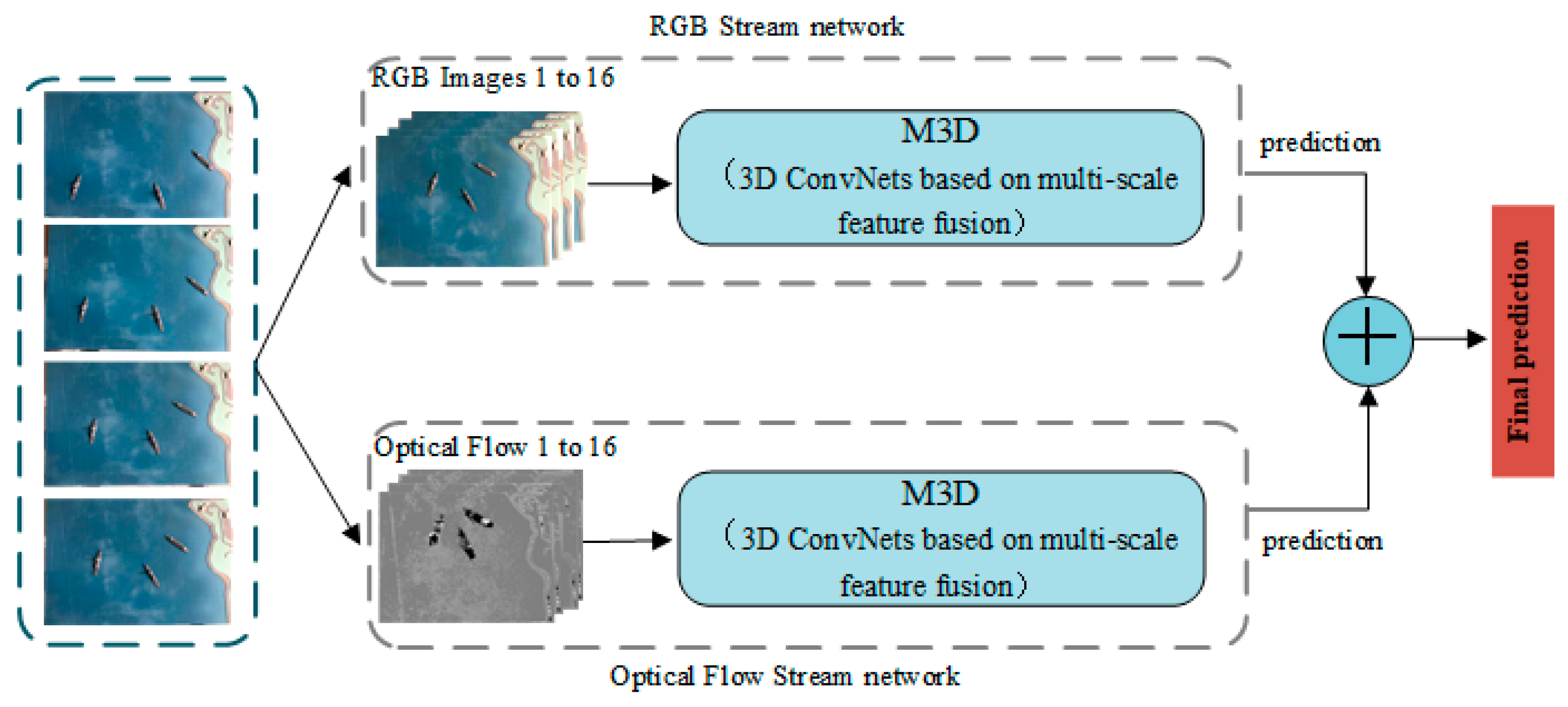
Battlefield target aggregation is a kind of behavior which can be regarded as the process of the combat units gathering from the starting position to the target, with obvious temporal and spatial characteristics. In this paper, we have proposed a new ConvNet called 3D convolution Two-Stream model based on multi-scale feature fusion. As shown in Figure 1, the 3D ConvNets based on multi-scale feature fusion (M3D) extracts the features of RGB sequences and optical flow sequences respectively, and obtains recognition results by averaging the output of the two networks.

The RGB network is a deep learning network that performs behavior recognition by extracting the spatio-temporal information of multi-frame RGB images.

The input of the optical flow network is a sequence of optical flow images that contains motion information. Although RGB images can provide rich exterior information, they are likely to cause background interference. Optical flow images can shield background interference, which helps the network understand the motion information of the target. Therefore, the optical flow network can effectively pay attention to the motion information in the video. The backbone network of this paper adopts a modular design, and the main body is composed of multi-fiber modules.

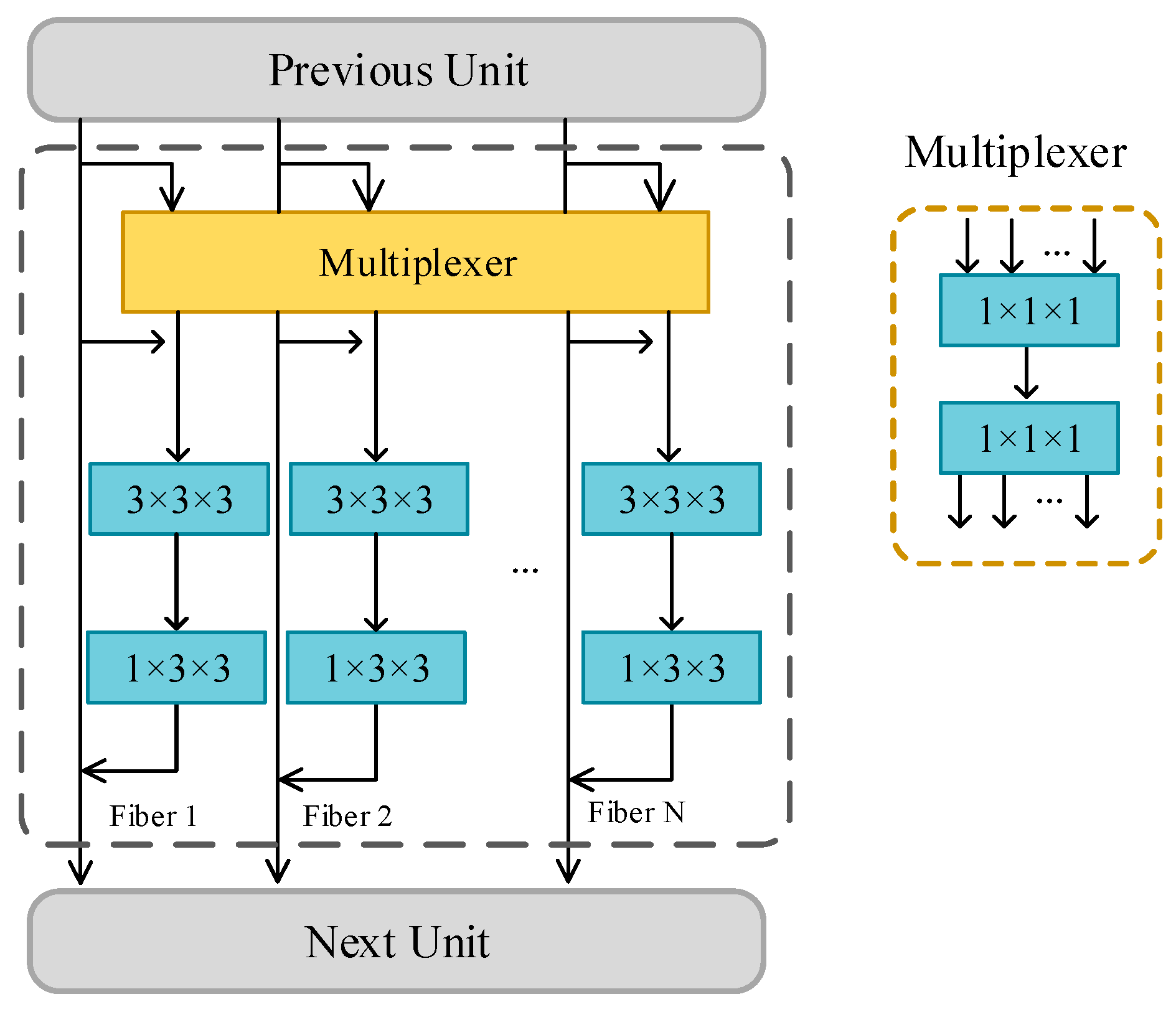
3.1. Multi-Fiber Unit (MF Unit)

In order to reduce the computational cost and increase the depth of the network, we use the improved spatio-temporal multi-fiber network as the backbone network. The calculation amount of the network is closely related to the number of connections between the two layers. The traditional conventional unit uses two convolutional layers to learn features, which is straightforward but computationally expensive. The total number of connections between these two layers can be computed as:

$$C=(M_{in}\times M_{mid}+M_{mid}\times M_{out}),$$

(1)

where $C$ represents the connections, $M_{in}$ represents the number of input channels, $M_{mid}$ represents the number of middle channels and $M_{out}$ represents the number of output channels.

Equation (1) indicates that the number of network connections is the quadratic of the network width.

The spatio-temporal multi-fiber convolution network is modular in design, with the multi-fiber unit splitting a single path into N parallel paths, each path being isolated from the other paths. As shown in Equation (2), the total width of the unit remains the same, but the number of connections is reduced to the original 1/N. In this paper, we set N = 16.

$$C=N\times (\frac{M_{in}}{N}\times \frac{M_{mid}}{N}+\frac{M_{mid}}{N}\times \frac{M_{out}}{N})=\frac{(M_{in}\times M_{mid}+M_{mid}\times M_{out})}{N}$$

(2)

The multiplexer can share information between N paths. The first 1 × 1 × 1 convolutional layer is responsible for merging the features and reducing the number of channels, and the second 1 × 1 × 1 convolution layer distributes the feature map to each channel. The parameters within the multiplexer are randomly initialized and automatically adjusted by end-to-end backpropagation. The multi-fiber module and multiplexer are shown in Figure 2.

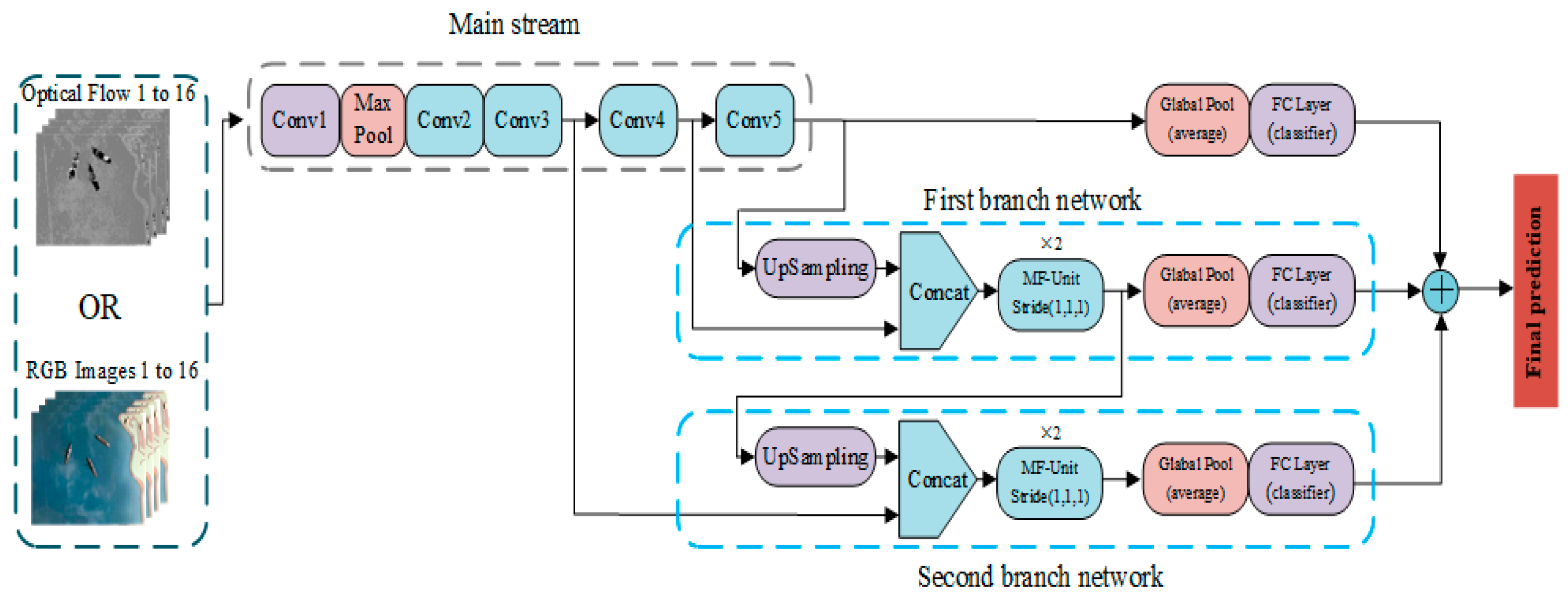
3.2. 3D ConvNets Based on Multi-Scale Feature Fusion (M3D)

As shown in Figure 3, 3D ConvNets based on multi-scale feature fusion (M3D) consists of a mainstream network and two tributary networks. The input size of the mainstream network is 16 × 224 pixels × 224 pixels. The network settings are shown in

Table 1. Mainstream network settings. When the input is an optical flow frame, the number of input channels of the network is 2. When the input is an RGB image, the network input channel is 3. The stride is denoted by “(temporal stride, height stride, and width stride)”.

Layer	Repeat	Channel	Stride	Output Size
Input		3(RGB)/2(Flow)		16 × 224 × 224
Conv1	1	16	(1, 2, 2)	16 × 112 × 112
MaxPool		16	(1, 2, 2)	16 × 56 × 56
Conv2_X (MF Unit)	3	96	(1, 1, 1)	16 × 56 × 56
Conv3_X (MF Unit)	1	192	(2, 2, 2)	8 × 28 × 28
	3		(1, 1, 1)
Conv4_X (MF Unit)	1	384	(2, 2, 2)	4 × 14 × 14
	5		(1, 1, 1)
Conv5_X (MF Unit)	1	768	(2, 2, 2)	2 × 7 × 7
	2		(1, 1, 1)
AvgPooling				1 × 1 × 1
FC				2

. We carry out the spatio-temporal down-sampling in Conv5_1, Conv3_1 and Conv4_1 with stride (2, 2, 2). In Conv1 and MaxPool, the down-sampling of the spatio was carried out, and the stride is (1, 2, 2). The output of Conv5_3 is the averaged spatio-temporal pooling, and results in all kinds of recognition probabilities through the fully connected layer.

In the process of multi-scale feature map fusion, it must be ensured that the multi-scale feature can retain the original information after fusion and maintain the validity of the fusion feature. In view of the above situation, this paper proposes a number of fusion methods, and the function is expressed as:

$$y=f(x^a,x^b),$$

(3)

where $x^a\in P^{t\times h\times w}$ and $x^b\in P^{\prime }{}^{t\times h\times w}$ represent the two-layer feature map that is to be fused. $y\in P^{″}{}^{t\times h\times w}$ represents the merged feature map, $t$ represents the number of frames, and $h$, $w$ represent the height and width, respectively, of the corresponding feature map.

Concatenation. Cascading the feature maps of two 3D convolutional layers. This can be represented as Equation (4):

$$\{\begin{array}{l}{y}_{i,j,2k}^{cat}=x_{i,j,k}^a\\ y_{i,j,2k+1}^{cat}=x_{i,j,k}^b\end{array}1\le i\le h;1\le j\le w;1\le k\le t,$$

(4)

where $(i,j,k)$ represents a coordinate point in the feature map.

Sum. Adding the elements of the same coordinate point in the two feature maps. This can be represented as Equation (5):

$$y_{i,j,k}^{\mathrm{sum}}=x_{i,j,k}^{\mathrm{a}}+x_{i,j,k}^{\mathrm{b}}$$

(5)

Maximum. Take the larger of the same coordinate points in the two feature maps. This can be represented as Equation (6):

$$y_{i,j,k}^{\max }=\max \{x_{i,j,k}^{\mathrm{a}},x_{i,j,k}^{\mathrm{b}}\}$$

(6)

Average. Calculate the mean of the same coordinate points in the two feature maps. This can be represented as Equation (7):

$$y_{i,j,k}^{\mathrm{ave}}=(x_{i,j,k}^{\mathrm{a}}+x_{i,j,k}^{\mathrm{b}})/2$$

(7)

It is worth noting that the three methods of sum, maximum and average do not change the number of channels. Although the cascade fusion increases the number of channels of the feature map, the information volume of each channel is not compressed. Therefore, the cascading fusion is more conducive to retaining the original information.

4. Building Dataset

4.1. Data Collection

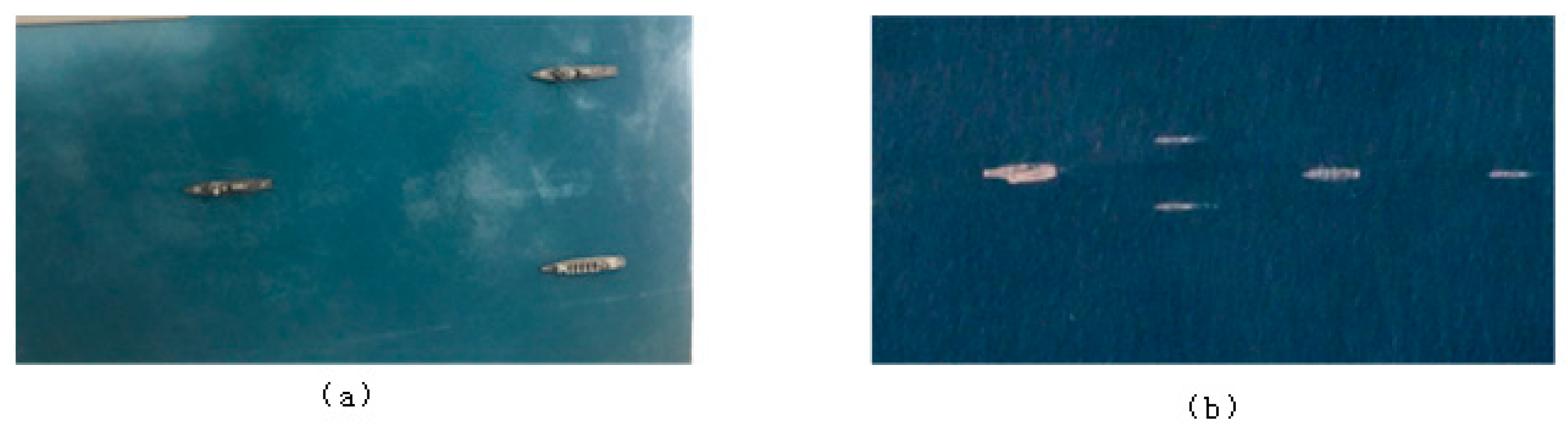
Due to the particularity of battlefield target aggregation behavior, intelligence videos are difficult to obtain. Our article does not consider the disturbances of complex environmental factors (such as complex weather, etc.). Therefore, we collected video data on a satellite simulation platform and built the dataset based on the video data. Behavioral simulation data needs to ensure a visual similarity and behavioral similarity as much as possible. In terms of visual similarity, based on the acquisition of the static images in the open network, Figure 4 shows that the simulated data set has a visual similarity with the real data. In terms of behavioral similarity, the aggregate behavior can be seen as the behavior of groups moving to a certain area. From the perspective of space, the aggregation behavior shows a relative position change in the battlefield space; from the perspective of time, the aggregation behavior is a time series of the density of the combat unit from low to high. The warships are not affected by the terrain, so the trajectory of each target in the gathering behavior is roughly a straight line. Therefore, the data of our simulation has a certain authenticity.

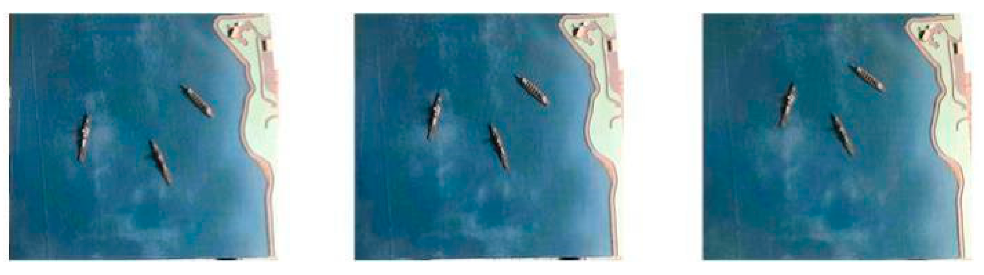
The purpose of this paper is to solve the binary classification problem of behavior. The dataset is divided into two categories: aggregation and others. The aggregate classes include behaviors such as dual-target aggregation and multi-target aggregation. Other classes include actions such as target static and target travel. The aggregate behavior class is the positive samples of model training. Other behavioral classes are negative samples of model training. In reality, in addition to the aggregation behavior, most of the behaviors captured in the video are target static, no target, and target travel (no aggregation trend), so the dataset constructed in this paper is representative. Part of the RGB training samples is shown in Figure 5.

According to the actual speed of 20 times, 1000 segments of the video are collected. Each video lasts for 30 to 40 seconds. The resolution of each video is 720 pixels × 480 pixels, and the frame rate is 25 fps. Our dataset consists of 500 aggregation behavior video and 500 other behavior videos. Each category is randomly divided into five splits, each containing 100 videos. The data set is shown in

Table 2. Experimental dataset. The dataset consists of 500 aggregation behavior videos and 500 other behavior videos. Each category is randomly divided into five splits, each containing 100 videos.

Category	Split1	Split2	Split3	Split4	Split5
Aggregation	100	100	100	100	100
Others	100	100	100	100	100

.

4.2. Optical Flow Video

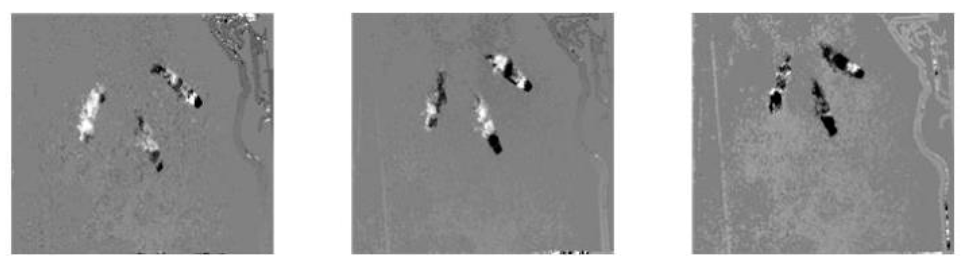
The optical flow can characterize the motion of the object. Using the optical flow data as the training data is beneficial to improving the recognition rate. On the one hand, the optical flow data can shield the interference of the complex background; on the other hand, the optical flow graph contains enough motion information, which can make the network more comprehensively learn aggregation behavior characteristics. The partial optical flow samples are shown in Figure 6.

4.3. Data Enhancement

When training deep networks, it is easy to over-fit due to insufficient labeling samples [20]. Data enhancement can effectively avoid over-fitting. This article uses two enhancement strategies for data. (1) In the video, we extract multiple times with different frames as the first frame, and the sampling interval is 30 frames. The extracted segments have 16 frames, and there is an overlap between the extracted segments; (2) Corner cropping. First, we scale the image size to 256 pixels × 256 pixels, and then crop from the center and 4 diagonal regions into 5 sub-images of 224 pixels × 224 pixels.

The experimental results show that the data enhancement improves the generalization ability of the network and improves the recognition accuracy.

5. Experimental Section and Analysis

5.1. Experimental Setup and Training Strategy

We tested our methods in the Ubuntu16.04 environment. The details are shown in

Table 3. Experimental configuration.

Operating System	Ubuntu16.04
CPU	Intel Core I9-7940X
GPU	Nvidia GeForce TITANV
Design language	Python3.5
Frame	Pytorch
CUDA	Cuda8.0

.

The training optimization of the RGB network and optical flow network is based on Back-propagation (BP). Our models are optimized with a vanilla synchronous SGD algorithm with the momentum of 0.9. The networks are trained with an initial learning rate of 0.1, which decays step-wisely with a factor of 0.1. The batch size of the dataset is 16, which is to say that the network has 16 segments per iteration, and the network reaches a steady state when iterating 6000 times. The optical flow is calculated by TVL1 of the OpenCV algorithm.

5.2. Multi-Scale Network Comparison Test

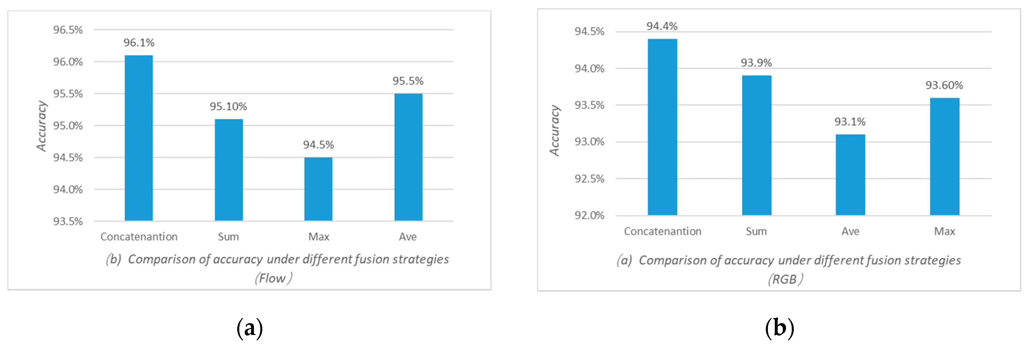
As shown in Figure 7, we compare the accuracy rates in different fusion methods. The fusion methods include Concatenation, Sum, Max, and Ave. The experimental results show that the fusion of concatenation has the highest recognition accuracy.

The two-stream convolutional network in this paper is divided into the RGB network and optical flow network. The network input is 16 frames of the RGB sequence or 16 frames of the optical stream sequence. In order to verify the advantages of this network framework in identifying accuracy and computational complexity, we tested the identification results of the networks in the dataset constructed in this paper. We use FLOPs (floating-point multiplication-adds) to measure the amount of computation.

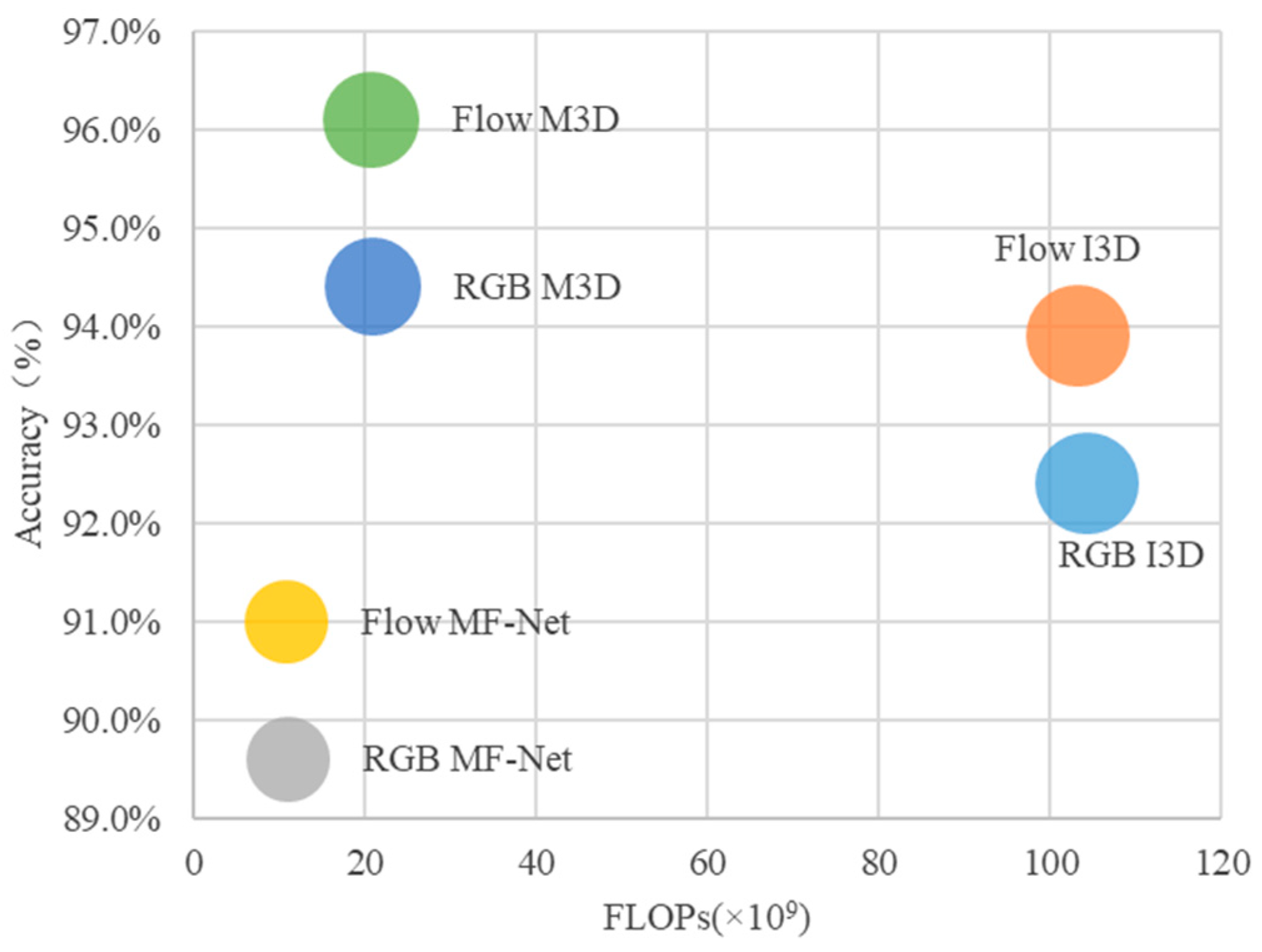
The experimental comparison method is the I3D [14] network (including the RGB tributary and optical stream tributaries) and MF-Net [18]. The experimental results are shown in

Table 4. Branch network comparison on the dataset constructed in this paper. Test1–5 represents the results of the first to fifth cross-validation tests.

Method	Test1	Test2	Test3	Test4	Test5	Average
RGB I3D	94.5%	90.5%	91.5%	92.5%	93%	92.4%
Flow I3D	95%	92%	93%	94.5%	95%	93.9%
RGB MF-Net	90%	89.5%	88.5%	91%	89%	89.6%
Flow MF-Net	91.5%	90.5%	90.5%	92.5%	90%	91%
RGB M3D (Ours)	96%	92.5%	94%	95%	94.5%	94.4%
Flow M3D (Ours)	97%	94%	95.5%	97.5%	96.5%	96.1%

and Figure 8. The M3D proposed in this paper achieves a 94.4% and 96.1% accuracy, respectively, when the input is the RGB sequence or the optical flow sequence. Comparing the three networks, the recognition results of the proposed algorithm are improved to different degrees than I3D and MF-Net. The experimental results show that: (1) Introducing multi-scale feature fusion into the 3D-CNN can effectively improve the accuracy of the network recognition. (2) The use of multi-fiber modules can greatly reduce the parameter amount and calculation expenses while ensuring the recognition accuracy.

5.3. Test of Two-Stream Network

In this section, the experimental results obtained by the M3D(RGB) and the M3D(Flow) are weighted and fused according to different weights, and then the optimal distribution ratio is selected. The results are shown in

Table 5. The accuracy of the Two-Stream network at different weight ratios, where the distribution ratio = M3D(RGB): M3D(Flow). Test1–5 represents the results of the first to fifth cross-validation tests.

Distribution Ratio	Test1	Test2	Test3	Test4	Test5	Average
3:7	97%	94.5%	95.5%	97.5%	96.5%	96.2%
4:6	97%	95.5%	96%	98%	97%	96.7%
5:5	98%	96.5%	96%	98.5%	97.5%	97.3%
6:4	96.5%	94%	95.5%	97%	96.5%	95.9%

, where the distribution ratio = M3D(RGB): M3D(Flow).

As shown in Table 5, when the distribution ratio is 5:5, the Two-Stream network of this paper achieves the best recognition rate. The recognition accuracy on the dataset constructed in this paper reached 97.3%.

5.4. Comparison of Various Methods

Table 6. Action recognition accuracy on the dataset constructed in this paper. Test1–5 represents the results of the first to fifth cross-validation tests. In the input, R means the input is RGB, R+OF means the input is RGB and Optical Flow. The Two-Stream M3D outperforms C3D by 13.3%, LSTM+CNN by 17%, Two-Stream I3D by 1.6%, and Two-Stream MF-Net by 5.1%.

Method	Inputs	Params	Test1	Test2	Test3	Test4	Test5	Average
LSTM+CNN	R	9M	82.5%	81%	77%	82%	79%	80.3%
C3D	R	79M	83%	84%	82.5%	85%	85.5%	84%
Two-Stream I3D	R+OF	23.4M	96%	94%	95%	97%	96.5%	95.7%
Two-Stream MF-Net	R+OF	16.9M	92.5%	92%	91.5%	94%	91%	92.2%
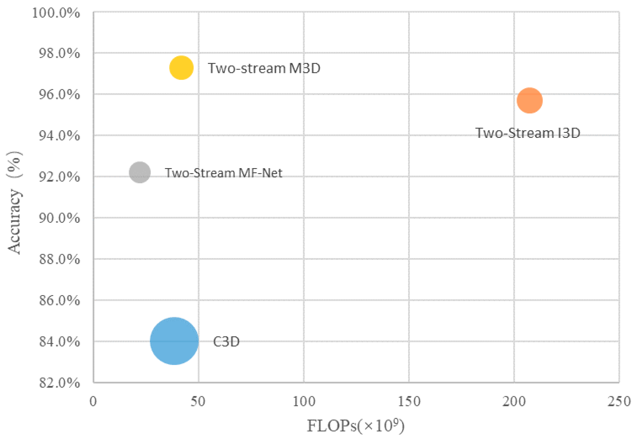
Two-Stream M3D	R+OF	20.9M	98%	96.5%	96%	98.5%	97.5%	97.3%

shows the video action recognition results of different models trained on the dataset established in this paper. It can be seen that: (1) From the perspective of the network structure, the algorithm combines different size feature maps, which is not available in other networks. The fusion of a multi-scale feature map compensates for the risk of the video information loss; (2) From the experimental results, compared with the traditional single-channel input network such as C3D [14], the accuracy of the two-stream M3D is improved by 13.3%. The main reason for this is that the multi-scale feature fusion strategy can more effectively extract spatio-temporal information. Compared with the LSTM+CNN [14], the accuracy of the Two-Stream M3D is improved by 17%. The main reason is that the LSTM (Long Short-Term Memory) on features from the last layers of ConvNets can model a high-level variation, but may not be able to capture fine low-level motion. Because CNN loses many fine-grained underlying features during down-sampling, these underlying features may be critical for a proper motion recognition. That is to say, the feature map outputted by CNN loses the information of smaller targets. If this feature map is input into LSTM for a timing analysis, the recognition result will be greatly affected. Compared with the two-stream network, the Two-Stream M3D proposed in this paper effectively improves the recognition accuracy, which is 1.6% and 5.1% higher than Two-Stream I3D and Two-Stream MF-Net, respectively. Figure 9 shows that the proposed model achieves a good trade-off between computational complexity and accuracy.

6. Conclusions

This paper was aimed at the problem of battlefield target aggregation behavior recognition based on intelligence videos: (1) This paper proposes the M3D model, which effectively reduces the impact of network down-sampling on the network recognition accuracy by combining different scale feature maps. The algorithm can effectively deal with the problem that the target of aggregation behavior is small and that the duration is uncertain; (2) Thanks to the multi-fiber module, our algorithm achieves a good trade-off between computational complexity and accuracy. On the established aggregation behavior dataset, the algorithm of this paper is experimentally verified and compared with several advanced algorithms. The results of multiple experiments show that the proposed algorithm can effectively improve the accuracy of the aggregation behavior recognition.

We have not yet verified the algorithm in a complex environment. Under realistic conditions, complex environmental factors will increase the difficulty of recognition of the algorithm. When the cloud is occluded or the visibility is low, the recognition fails because the target cannot be observed. For the ocean target, when the sea surface has a severe diffuse reflection, the optical flow images extracted by the traditional optical flow method will have a large noise, which is not conducive to the algorithm’s recognition of the behavior. In future work, in view of the feature extraction advantages of traditional algorithms in complex environments, we will start with a combination of traditional methods and deep learning to explore a more robust recognition algorithm.

References

- Huang, M.; Su, S.Z.; Cai, G.R.; Zhang, H.B.; Cao, D.; Li, S.Z. Meta-action descriptor for action recognition in RGBD video. IET Comput. Vis. 2017, 11, 301–308. [Google Scholar] [CrossRef]
- Peng, X.; Wang, L.; Wang, X.; Qiao, Y. Bag of visual words and fusion methods for action recognition: Comprehensive study and good practice. Comput. Vis. Image Underst. 2016, 150, 109–125. [Google Scholar] [CrossRef] [Green Version]
- Duta, I.C.; Ionescu, B.; Aizawa, K.; Sebe, N. Spatio-Temporal VLAD Encoding for Human Action Recognition in Videos. In Proceedings of the International Conference on the MultiMedia Modeling (MMM), Reykjavik, Iceland, 4–6 January 2017. [Google Scholar]
- Li, C.; Zhong, Q.; Xie, D.; Pu, S. Collaborative Spatio-temporal Feature Learning for Video Action Recognition. Available online: https://arxiv.org/pdf/1903.01197 (accessed on 14 May 2019).
- Zolfaghari, M.; Oliveira, G.L.; Sedaghat, N.; Brox, T. Chained Multi-stream Networks Exploiting Pose, Motion, and Appearance for Action Classification and Detection. In Proceedings of the IEEE International Conference on Computer Vision (ICCV), Venice, Italy, 22–29 October 2017. [Google Scholar]
- Wang, H.; Schmid, C. Action Recognition with Improved Trajectories. In Proceedings of the IEEE International Conference on Computer Vision (ICCV), Sydney, Australia, 8–12 April 2013. [Google Scholar]
- Simonyan, K.; Zisserman, A. Two-Stream Convolutional Networks for Action Recognition in Videos. Adv. Neural Inf. Process. Syst. 2014, 2, 111–119. [Google Scholar]
- Wang, L.; Xiong, Y.; Wang, Z.; Qiao, Y.; Lin, D.; Tang, X.; Van Gool, L. Temporal Segment Networks: Towards Good Practices for Deep Action Recognition. In Proceedings of the European Conference on Computer Vision (ECCV), Amsterdam, The Netherlands, 8–16 October 2016. [Google Scholar]
- Feichtenhofer, C.; Pinz, A.; Wildes, R.P. Spatiotemporal Residual Networks for Video Action Recognition. Neural Inf. Process. Syst. 2016, 29, 3468–3476. [Google Scholar]
- Feichtenhofer, C.; Pinz, A.; Wildes, R.P. Spatiotemporal Multiplier Networks for Video Action Recognition. In Proceedings of the IEEE Conference on Computer Vision and Pattern Recognition (CVPR), Honolulu, HI, USA, 22–25 July 2017. [Google Scholar]
- Zhu, Y.; Lan, Z.; Newsam, S.; Hauptmann, A.G. Hidden Two-Stream Convolutional Networks for Action Recognition. Available online: https://arxiv.org/pdf/1704.0389 (accessed on 14 May 2019).
- Donahue, J.; Anne Hendricks, L.; Guadarrama, S.; Rohrbach, M.; Venugopalan, S.; Saenko, K.; Darrell, T. Long-Term Recurrent Convolutional Networks for Visual Recognition and Description. TPAMI 2017, 39, 677–691. [Google Scholar] [CrossRef] [PubMed]
- Varol, G.; Laptev, I.; Schmid, C. Long-Term Temporal Convolutions for Action Recognition. IEEE Trans. Pattern Anal. Mach. Intell. 2018, 40, 1510–1517. [Google Scholar] [CrossRef] [PubMed]
- Carreira, J.; Zisserman, A. Quo Vadis, Action Recognition? In Proceedings of the IEEE Conference on Computer Vision and Pattern Recognition (CVPR), Honolulu, HI, USA, 22–25 July 2017. [Google Scholar]
- Qiu, Z.; Yao, T.; Mei, T. Learning Spatio-Temporal Representation with Pseudo-3D Residual Networks. In Proceedings of the IEEE International Conference on Computer Vision (ICCV), Venice, Italy, 22–29 October 2017. [Google Scholar]
- Xie, S.; Sun, C.; Huang, J.; Tu, Z.; Murphy, K. Rethinking Spatiotemporal Feature Learning: Speed-Accuracy Trade-offs in Video Classification. In Proceedings of the European Conference on Computer Vision (ECCV), Munich, Germany, 8–14 September 2018; pp. 305–321. [Google Scholar]
- Tran, D.; Wang, H.; Torresani, L.; Ray, J.; LeCun, Y.; Paluri, M. A Closer Look at Spatiotemporal Convolutions for Action Recognition. In Proceedings of the IEEE Conference on Computer Vision and Pattern Recognition (CVPR), Salt Lake City, UT, USA, 19–21 June 2018. [Google Scholar]
- Chen, Y.; Kalantidis, Y.; Li, J.; Yan, S.; Feng, J. Multi-Fiber Networks for Video Recognition. In Proceedings of the European Conference on Computer Vision (ECCV), Munich, Germany, 8–14 September 2018. [Google Scholar]
- Lin, T.Y.; Dollar, P.; Girshick, R.; He, K.M.; Hariharan, B.; Belongie, S. Feature Pyramid Networks for Object Detection. Available online: https://arxiv.org/pdf/1612.03144 (accessed on 14 May 2019).
- Qu, L.; Wang, K.R.; Chen, L.L.; Li, M.J. Fast road detection based on RGBD images and convolutional neural network Acta Optica Sinica. Acta Opt. Sinica 2017, 37, 1010003. [Google Scholar]
Figure 1.
Two-Stream M3D (3D convolution Two-Stream model based on multi-scale feature fusion). M3D (3D ConvNets based on multi-scale feature fusion) extracts the features of RGB (Red-Green-Blue) sequences and optical flow sequences respectively, and gets the recognition results by averaging the output of the two networks.
Figure 2.
Multi-fiber unit and multiplexer. The multiplexer module was incorporated to facilitate the information flow between the fibers.
Figure 3.
Network architecture details for M3D. The input of the first branch is the output of Conv5_3 and Conv4_6. The input of the second branch is the output of the first branch convolution module and the output of Conv3_4. The classification probability of the three-way network is averaged to obtain the final recognition probability. In the first branch network, in order to splice the output feature maps of Conv5_3 and Conv4_6, we use the up-sampling layer to up-sample the feature map of Conv5_3 from 4 × 7 × 7 to 8 × 14 × 14. The spliced feature map is sent to the convolution module to extract the features, and after the pooling layer the full connection layer obtains the classification probability of the branch. In the second branch network, with the first branch network feature map, we up-sample the spatio-temporal resolution by a factor of 2 (using nearest neighbor up-sampling for simplicity). The up-sampled map is then merged with the feature map of Conv3_4. The spliced feature map is sent to the convolution module to extract the features and results in the classification probability after the fully connected layer. Finally, the classification probability of the three-way network is averaged to obtain the final recognition probability.
Figure 4.
(a) Simulation data. (b) Real data. Visually speaking, the background and the shape of the object are similar.
Figure 5.
Dataset RGB sample. The above pictures show a few frames extracted from a video clip.
Figure 6.
Dataset optical flow sample. The optical flow image is obtained by calculating the optical flow between two frames of the RGB images.
Figure 7.
(a) Accuracy of optical flow branches under different fusion strategies. (b) Accuracy of RGB branches under different fusion strategies. We compared the accuracy rates in different fusion methods. The experimental result is the average of the results of 5-fold cross-validation tests. Concatenation works best because the concatenation method does not merge the channels and can retain the original information of the feature map.
Figure 8.
Efficiency comparison between different 3D convolutional networks on the dataset constructed in this paper. The computational complexity is measured using FLOPs, i.e., floating-point multiplication-adds. The area of each circle is proportional to the total parameter number of the model. FLOPs for computing the optical flow are not considered.
Figure 9.
Efficiency comparison between different methods. The computational complexity is measured using FLOPs, i.e., floating-point multiplication-adds. The area of each circle is proportional to the total parameter number of the model. FLOPs for the computing optical flow are not considered.