A Time-Space Network Model Based on a Train Diagram for Predicting and Controlling the Traffic Congestion in a Station Caused by an Emergency

1
Key Laboratory of Transport Industry of Big Data Application Technologies for Comprehensive Transport, Ministry of Transport, Beijing Jiaotong University, Beijing 100044, China
2
School of Transportation, Beijing Jiaotong University, Beijing 100044, China
*
Author to whom correspondence should be addressed.
Symmetry 2019, 11(6), 780; https://doi.org/10.3390/sym11060780
Submission received: 23 May 2019
/
Revised: 6 June 2019
/
Accepted: 10 June 2019
/
Published: 12 June 2019
(This article belongs to the Special Issue Symmetry in Engineering Sciences)
Abstract
:Timely predicting and controlling the traffic congestion in a station caused by an emergency is an important task in railway emergency management. However, traffic forecasting in an emergency is subject to a dynamic service network, with uncertainty surrounding elements such as the capacity of the transport network, schedules, and plans. Accurate traffic forecasting is difficult. This paper proposes a practical time-space network model based on a train diagram for predicting and controlling the traffic congestion in a station caused by an emergency. Based on the train diagram, we constructed a symmetric time-space network for the first time by considering the transition of the railcar state. On this basis, an improved A* algorithm based on the railcar flow route was proposed to generate feasible path sets and a dynamic railcar flow distribution model was built to simulate the railcar flow distribution process in an emergency. In our numerical studies, these output results of our proposed model can be used to control traffic congestion.
1. Introduction
1.1. The Description of the Subject of Research and the Motives to Take
When the station in a transportation network stops operation due to natural disasters and other emergencies, trains cannot pass through the station. Thus, trains arriving or passing through the station have to be rerouted. As there are capacity limitation stations in the transportation network, after a period of time, the railcar flow in some of the other stations will become overstocked, thus forming congestion. The congestion will greatly reduce the network’s transport capacity. Failure to timely predict the congestion will result in propagation of congestion and even the paralysis of the transportation network.
Effectively predicting and controlling the traffic congestion in a station caused by an emergency must have the following characteristics:
- Strong timeliness. Because of the transmissibility of congestion, it is of great significance to predict congestion in time for maintaining and improving the capacity of the transport network in an emergency.
- Time-space. The final output of the model should be which station will become congested first and when the station begins to become congested. These output results will become the basis of the decision of the railway transportation managers.
- Strongly controllable. Rail transportation is a strongly controlled mode of transport, which means that the turnover process of railcar flow and the distribution of railcar flow in the transport network are subject to schedules and plans.
- Multiple highly dynamic constraints. Congestion prediction and control in an emergency is a complicated system involving many components. First, the capacity in the network will be reduced in an emergency. Second, the state of railcar flow will change dynamically with the operation process and the state of some railcar flows changes more than twice within the decision-making period horizon. Third, the completion rate of the transportation plan and scheduled train departure will be affected by the emergency.
Congestion prediction and control problem is a new research field with strong exploration, which is not only the premise of rational utilization and enhancement of transport capacity, but also the premise of adjustment of rail transit. However, large-scale railcar flow, the complex railcar flow turnover process, and dynamic constraints (schedule constraints, loading plan constraints, emptying plan constraints, capacity constraints) make congestion prediction and control in an emergency very difficult.
To summarize, reasonable prediction and control of traffic congestion in a station caused by an emergency has already become a theoretically and practically urgent problem.
1.2. Literature Review
Recent research efforts have shown the ability to model congestion prediction and control of road transportation [1,2,3,4,5] and the metro [6,7,8,9,10]. Sun et al. [11] explored the hazardous materials route problem in the road-rail multimodal transportation network with a hub-and-spoke structure. Jiang et al. [12] proposed an emergency material vehicle dispatching and routing model which has multi-objective and multi-dynamic-constraint. Lu et al. [13] presented an approach to measure and analyze the vulnerability of urban rail transit network based on accessibility, which explicitly considers the characteristics of rail transit passenger flow, travel cost changes and alternative modes of transportation. Deng et al. [14] designed for passenger bus bridge circuit in the case of urban rail traffic interruption. The results of these models have provided a basis for emergency traffic control planning and evacuation order in time for transportation disruptions caused by equipment failures, accidents, peak traffic, and natural disasters.
The core problem of prediction and control of traffic congestion in a station caused by an emergency is the railcar management problem (this problem mainly concerns the distribution of railcar flow in the transportation network). White et al. [15] generated the network from the time-space graph and solved the transshipment problem by using the improved out-of-kilter algorithm. Static formulations solvable as transportation problems were proposed by Allman et al. [16]. Spieckermann et al. [17] formulated the problem of empty railcar assignment as a scheduling problem with machine to represent railcar and job to represent railcar process request. Holmberg et al. [18] proposed a multi-commodity network flow model for operational distribution of empty railcars. Narisetty et al. [19] proposed an optimization model to implement the union Pacific railway (UP) to allocate empty freight railcars based on demand. Gorman et al. [20] discussed the practice of optimizing the allocation of empty freight railcars for shippers by BNSF and CSX, two major U.S. freight companies. Heydari et al. [21] proposed a new solution to the problem of empty railcars distribution, which not only meets the needs of customers, but also takes into account the practical technical and business needs. Jiang et al. [22] proposed an integrated scheduling coordination model, which aimed to maximize the production connection time (PCT) and production delivery time (PDT). Sun et al. [23] explored the impact of demand uncertainty on the problem of the run-level cargo path of the multi-modal transport network based on rail transit based on time arrangement and road traffic based on time flexibility. Aiming at the design problem of railway express freight service network, Lin et al. [24] proposed a bi-level programming model, and transformed the lower-level model into a linear model by using linearization technology, which can be solved directly by standard optimization solver. Lawley et al. [25] proposed a time-space network flow model for scheduling regular bulk rail traffic from suppliers to customers. Sayarshad et al. [26] proposed a solution to optimize the fleet size and the configuration of freight railcars under uncertain demand conditions. However, the traditional railcar management model such as the empty railcar distribution model does not consider the transition of the railcar state (empty railcar to loaded railcar and loaded railcar to empty railcar) [27]. The comparisons between a few published studies on the railcar management model and this work are presented in Table 1. The innovation points of this paper are as follows:
- Based on the train diagram, we constructed a time-space network for the first time by considering the transition of the railcar state.
- The problem is split into two sub-problems: feasible path set generation and railcar flow distribution. An improved A* algorithm based on railcar flow route was used to generate a feasible path set of any pair of transportation demands. A dynamic railcar flow distribution model in an emergency which can be solved by mathematical programming software was established to simulate the process of railcar flow operation in emergency, and the railcar flow distribution in the future period was estimated based on the distribution results of railcar flow in the time-space network, so as to predict where there will be traffic congestion and when the traffic congestion will begin in the station.
The paper is organized as follows: Section 1 introduces the subject of research and the motives to take, and provides a brief survey of the literature devoted to the congestion prediction and control problem. In Section 2, we describe the congestion prediction and control problem in detail. In Section 3, an improved A* algorithm based on railcar flow route and a dynamic railcar flow distribution model in emergency are proposed. Section 4 and Section 5 present a numerical example and conclusion respectively.
2. Problem Description
In this section, first, we describe the process resulting in traffic congestion in a station due to the emergency to illustrate the need for timely predicting and controlling the traffic congestion. Then, we analyze the turnover process of railcar and transition of the railcar state in detail. Finally, we abstract the railcar management problem into a multi-commodity flow problem.
2.1. The Process Resulting in Traffic Congestion due to the Emergency
We describe the process resulting in traffic congestion due to the emergency in Figure 1. There are five normal stations and two railcar flow types (a railcar flow type refers to a class of railcar flows with the same origin station, destination station, and flow route) in period 1. In period 2, station B is interrupted due to an emergency, so the railcar flows with type 1 have to adjust the transport path. When a large number of railcar flows of type 1 and type 2 converge at station C simultaneously, it is likely that the number of real-time railcars in station C exceeds the capacity of the station, thus forming traffic congestion in period 3. For both types of railcar flows, the two paths to be traveled are blocked, which will result in the accumulation of railcars at station B and station A in period 4. Stations A and B become congested stations when the number of accumulated railcars exceeds their capacity. The propagation of congestion will greatly decrease the station capacity and transportation efficiency, therefore, it is of great significance to predict and control the traffic congestion in time.
2.2. The Turnover Process of Railcar and Transition of Railcar State
The railcar flow (a railcar flow refers to a collection of railcars with the same railcar flow type and generated in the same period) starts from the origin station and ends at the destination station through various transfer stations. As shown in Figure 2, each railcar flow is assigned into different trains along the way and each railcar flow can go through 11 activities, including train arrival, train break-up, loaded railcar delivery, empty railcar delivery, railcar loading, railcar unloading, loaded railcar pickup, empty railcar pickup, railcar assembly, train formation, and train departure. The implications of these 11 activities are as follows:
- Train arrival. The activity begins when the inbound train carrying railcars arrives at the station’s receiving yard and ends when railcars detached from the inbound train are pushed over the top of the station’s hump.
- Train break-up. The activity begins when the railcars starts to slide off the hump and ends when all railcars detached from the inbound train roll down to the appropriate track in the station’s switchyard.
- Loaded railcar delivery. The activity begins when all loaded railcars detached from the inbound train roll down to the station’s switchyard and ends when the loaded railcars are pulled to the freight yard by the local locomotive.
- Empty railcar delivery. The activity begins when all empty railcars detached from the inbound train roll down to the station’s switchyard and ends when the empty railcars are pulled to the freight yard by the local locomotive.
- Railcar loading. The activity begins when all empty railcars detached from the inbound train start to load in the freight yard and ends when the empty railcars have finished loading the goods.
- Railcar unloading. The activity begins when all loaded railcars detached from the inbound train start to unload in the freight yard and ends when the loaded railcars have finished unloading the goods.
- Loaded railcar pickup. The activity begins when the loaded railcars detached from the inbound train start to hang to the local locomotive and ends when all the loaded railcars are pulled back to the station’s switchyard from the freight yard by the local locomotive.
- Empty railcar pickup. The activity begins when the empty railcars detached from the inbound train start to hang to the local locomotive and ends when all the empty railcars are pulled back to the station’s switchyard from the freight yard by the local locomotive.
- Railcar assembly. The activity begins when all railcars detached from the inbound train are pulled back to the station’s switchyard from the freight yard and ends when the railcars are able to form an outbound train.
- Train formation. The activity begins when the railcars detached from many inbound trains are able to form an outbound train and ends when the formation of an outbound train is completed.
- Train departure. The activity begins when the formation of an outbound train is completed and ends when the outbound train carrying railcars starts from the departure yard.
The operation process of a railcar flow is different in its origin station, transfer station, and destination station. The state of each railcar flow changes at the departure and destination stations, but does not change at the transfer stations. The processes of a railcar flow in different stations are as follows:
- Origin station. The operation processes of a railcar flow mainly include the initialization process of loaded railcar flow and the initialization process of empty railcar flow. The initialization process of empty railcar flow consists of railcar unloading, empty railcar pickup, railcar assembly, train formation, and train departure. The process realizes the transition of loaded railcar flow into empty railcar flow. The initialization process of loaded railcar flow consists of railcar loading, loaded railcar pickup, railcar assembly, train formation, and train departure. The process realizes the transition of loaded railcar flow into empty railcar flow.
- Transfer station. The main operation process is the transfer process of railcar flow. The transfer process of railcar flow consists of train arrival, train break-up, railcar assembly, train formation, and train departure.
- Destination station. The operation processes of a railcar flow mainly include the local operation process of loaded railcar flow, the secondary operation process, the local operation process of empty railcar flow, the empty railcar allocation process, and the formation and departure process. The local operation process of loaded railcar flow consists of train arrival, train break-up, loaded railcar delivery, and railcar unloading. The secondary operation process is the process of reloading for the loaded railcar after unloading. The local operation process of empty railcar flow consists of train arrival, train break-up, empty railcar delivery, and railcar loading. The empty railcar allocation process consists of empty railcar pickup, railcar assembly, train formation, and train departure. The formation and departure process consists of loaded railcar pickup, railcar assembly, train formation, and train departure. The local operation process of loaded railcar flow realizes the transition of loaded railcar flow into empty railcar flow. The secondary operation process and the local operation process of empty railcar flow realize the transition of loaded railcar flow into empty railcar flow.
2.3. Problem Abstraction
Kwon et al. [28] defined the railcars dispatching process as the blocks and sequences of railcars s that are scheduled to continue moving, as well as the stations where the railcar will be taken and started during its travel. In addition, they formulated the railcar management problem as a multi-commodity flow problem on a transport network.
We abstract the transportation process of railcar flow in the railroad network into the service network with time attributes. The loaded railcar flow has a fixed origin station and destination station in the transportation process, and cannot be separated [29,30]. Therefore, each loaded railcar flow can be regarded as a commodity in the service network, so the loaded railcar flow management problem can be regarded as a multi-commodity flow problem [31]. The empty railcar flow does not have a fixed origin station and destination station in the transportation process. However, the empty railcar flow comes from the loaded railcar flow after unloading and is consumed by converting to the loaded railcar flow after loading, so the empty railcar flow can also be regarded as a commodity in the service network. In this paper, we abstracted the railcar management problem into a multi-commodity flow problem.
3. Methods
The flowchart of predicting traffic congestion in a station in an emergency is shown in Figure 3. We disassemble the railcar management problem into two sub-problems. One of the sub-problems is the construction of a time-space network based on the turnover process of railcar and transition of railcar state, the other sub-problem is the construction of a dynamic railcar flow distribution model in an emergency. Based on the solution results of the model, we can calculate the real-time number of railcars at each station in each period. Finally, the congested station is determined by comparing the real-time number of railcars at the station and the storage capacity of the station.
We define each OD as a set of railcars flow which has the same origin station and destination station.
3.1. Construction of time-space Network Based on the Train Diagram
In order to simplify the scale of the problem, a railway bureau is taken as the research object, and the marshaling station, district station, large freight station, and boundary station of the railway bureau are taken as the main fulcrum stations, while the railcar flow of the intermediate station is merged in accordance with the section center rule [32]. Set the fulcrum station set in the railway bureau as S, and define the time-space network as G = (N, A), where N denotes the set of nodes and A denotes the set of arcs in the network. The network takes 18:00 of the current day to 18:00 of the next day as a decision cycle. The train diagram is the main frame of constructing the time-space network.
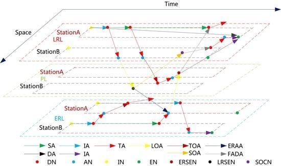
Network G takes the Arrival Node (AN) and Departure Node (DN) of as the main time-space nodes. The AN represents the arrival moment of a train and the DN represents the departure moment of a train. The Loaded Railcar State End Node (LRSEN) and the Empty Railcar State End Node (ERSEN) represent the mutual transformation moment of loaded railcar flow and empty railcar flow. Secondary Operation Completion Node (SOCN) represents the completion moment of secondary operation of loaded railcar flow. Each station sets two Initial Nodes (IN), which are divided into loaded railcar layer and empty railcar layer, to represent the start moment of the railcar flow in the decision cycle. Each station sets two End Nodes (EN), which are also divided into loaded railcar layer and empty railcar layer, to represent the end moment of the railcar flow in the decision cycle. The type indexes of time-space nodes are shown in Table 2.
Network G takes the train as the Train Arc (TA), and adds the corresponding Local Operation Arc (LOA) and Secondary Operation Arc (SOA) based on the technical operation time of each fulcrum station, and realizes the connection of each arc through the Formation and Departure Arc (FADA), Empty Railcar Allocation Arc (ERAA), Transfer Operation Arc (TOA), and Stay Arc (SA). The Initial Arc (IA) represents the initialization process of the railcar flow. The End Arc (EA) and the Detention Arc (DA) represent the process of railcar flow detention to the end of the decision cycle. At the same time, hierarchy attributes were added to distinguish the Loaded Railcar Layer (LRL), Empty Railcar Layer (ERL), and Public Layer (PL). At present, the research on dynamic railcar flow operation lacks the consideration of the secondary operation of the loaded railcar flow, and this paper represents the secondary operation process of the loaded railcar flow through the connection between LRSEN and SOCN. The network topology relationship between time-space nodes and time-space arcs is shown in Figure 4. The type indexes of time-space arcs are shown in Table 3 and the hierarchy indexes of the hierarchy set are shown in Table 4.
Because loaded railcar flow has the characteristics of a tree path, this paper describes the transport process of loaded railcar flow by constructing a time-space path which is a set of time-space arcs that satisfy the constraint of time continuity. The time-space path of loaded railcar flow is divided into four categories: Initial Path (IP), Secondary Operation Path (SOP), Empty to Loaded Path (ETLP), and Detention Path (DP). The IP represents the transport process of the initial loaded railcar flow. The path starts from the IN and ends at the LRSEN. The path takes the LOA as the final arc. The SOP represents the transport process of secondary operation loaded railcar flow. The path starts from the LRSEN and ends at the ETN. The path takes the SOA as the first arc and cannot contain the LOA. ETLP represents the transport process of self-loading railcar flow. The path starts from the ERSEN and ends at the EN. The DP representing the loaded railcar flow remains at the station throughout the decision cycle. The path starts from the IN and ends at the EN. The type indexes of time-space paths are shown in Table 5.
3.2. Feasible Path Set Generation Algorithm Based on Improved A* Algorithm
According to the requirements of a train marshaling plan, each OD (a set of railcars flow which has the same origin station and destination station) has a fixed railcar flow connection mode, thus each OD has a specific route, that is, the railcar flow route. In this paper, the feasible path has a broader meaning in the time-space network. For each OD, a set of time-space arc sets that satisfies the time continuity constraint and the constraint of the railcar flow route station sequence is a feasible time-space path.
A* algorithm is an efficient algorithm for solving K-shortest path [33,34,35]. We improve the algorithm based on the railcar flow route. Set OD index as f, the flowchart of improved A* algorithm is shown in Figure 5 and the algorithm for generating the feasible path set is as follows:
Step 1: Take f = 1, and turn to Step 2;
Step 2: Set the maximum index of K-shortest path of demand f to N, and initial K = 0, set the starting station of demand f as station1, and the final station as station2. Traverse the railcar flow route set, find the railcar flow route of the starting station as station1 and ending station as station2, and record the station sequence corresponding to the railcar flow route as station-list, and turn to Step 3;
Step 3: Taking the EN corresponding to station2 as the source node, the Dijkstra algorithm is used to find the shortest distance between the source node and other nodes in the time-space network, which is taken as the H value of each node, and turn to Step 4;
Step 4: Establish a node set as close-list which has been estimated and a node set as open-list which will be estimated. Add the IN corresponding to the station1 to the open-list, and turn to Step 5;
Step 5: Traverse the nodes in the open-list to find the node with the lowest F value and treat it as m to be processed, and turn to Step 6;
Step 6: Move this node from the open-list to the close-list, and turn to Step 7;
Step 7: For each pointing node of m as n, set its parent node as m, and recalculate its G and F values, and add them to the open-list, and turn to Step 8;
Step 8: If the open-list is empty, the target K short path is not found, and the search fails, then f = f + 1, and turn to Step 2. If the open-list is not empty, traverse the open-list, if the node with the lowest F value is the EN corresponding to station2, the target K shortest path is found, then K = K + 1, and turn to Step 9; otherwise turn to Step 5;
Step 9: First, judge whether K is greater than N, if K is greater than N, f = f + 1, then turn to Step 2. Otherwise, judge the number of LOA in the K shortest path. If the number is greater than 1, remove the K short path and turn to Step 4; if the number is equal to 1, divide the K short path into two paths with the end node of the LOA as the cutting node, and turn to Step 10;
Step 10: Take the station sequence of these two paths as station-list1 and station-list2. Determine whether the station sequence of each path is the same as the station-list, and if so, add the path to the feasible path set, and turn to Step 5;
Step 11: When all OD demands are traversed to generate a feasible path set, the algorithm is finished.
3.3. The Dynamic Railcar Flow Distribution Model in an Emergency
The key to predict the traffic congestion is to grasp the real-time number of railcars at a station. The train runs according to the train diagram, and the time-space network constructed based on the train diagram conforms to the situation of railway field operation. In this paper, based on the time-space network, the distribution results of railcar flow on the time-space network are obtained by establishing the dynamic railcar flow distribution model in an emergency. According to the arc flow, the real-time number of railcars at each station can be obtained. By comparing the real-time number of railcars at each station with the storage capacity of the station, it can be concluded whether the station belongs to the congestion stage, so as to be able realize the prediction of traffic congestion in the station.
3.3.1. Set Parameter and Variable Definitions
The general notations used in the formulation are listed in Table 6.
3.3.2. Objective Function
The objective is to compress the transit time of the loaded railcars at the station, reduce the running time of the empty railcars, and minimize the number of off-axle railcars. The expression is as follows:
3.3.3. Constraint Conditions
Initial loaded railcar flow constraints: For each loaded railcar flow, the sum of the number of flows allocated on the feasible path is equal to the number of initial loaded railcar flows.
Initial empty railcar flow constraints: For each empty railcar flow, the sum of the number of flows allocated on the feasible arc is equal to the number of initial empty railcar flow.
Consistent constraints of decision variables: For each IP or DP, the sum of the number of initial loaded railcar flows allocated on that path is equal to the number of flows of that path; for each IA or DA, the sum of the number of initial empty railcar flows allocated on that arc is equal to the number of flows of that arc.
Time-space arc capability constraints: For each time-space arc, the sum of the number of loaded railcar flows on that arc and the number of empty railcar flows on that arc cannot exceed the capacity of that arc.
Consistent constraints of exchange of LRL and ERL: For each LRSEN, the loaded railcar flow number of the IP ending at that node is equal to the sum of the loaded railcar flow number of the SOP starting from that node and the empty railcar flow number of the ERAA starting from that node. For each ERSEN, the empty railcar flow number of the LOA ending at that node is equal to the sum of the loaded railcar flow numbers of the ETLP starting from that node.
Flow conservation constraints of node in ERL: For each time-space node in ERL or PL, the sum of the empty railcar flow number of the time-space arc ending at that node in ERL or PL is equal to the sum of the empty railcar flow number of the time-space arc starting from that node in ERL or PL.
Loading plan constraints: For each loading plan, the sum of the loaded railcar flow number of the time-space paths in line with the loading plan cannot exceed the planned loading number for one day of the plan, nor can it be lower than the completed loading number of the plan when an emergency occurs.
Emptying plan constraints: For each emptying plan, the sum of the empty railcar flow number of time-space arcs in line with the emptying plan cannot exceed the planned emptying number for one day of the plan, nor can it be lower than the completed emptying number of the plan when an emergency occurs.
Train operation restrictions constraints in an emergency: For each affected TA, the sum of the number of loaded railcar flow on that arc and the number of empty railcar flow on that arc is equal to zero.
3.3.4. Model Synthesis
By combining constraints (1) to (12), the Dynamic Railcar Flow Distribution Model in an emergency (DRFDMUE) can be obtained.
DRFDMUE:
s.t.
Change constraint (10) and constraint (11) into constraint (13) and constraint (14) as follows:
Combining constraints (1) to (9), together with constraint (13) and constraint (14), the Dynamic Railcar Flow Distribution Model under Normality (DRFDMUN) can be obtained.
DRFDMUN:
s.t.
3.3.5. Solution Method
The model is a pure integer linear programming, so it can be solved by a branch and bound algorithm [36]. We implement the algorithm by c# programming. We use branch and bound algorithm to search the solution space tree of the problem and each node can become an extension node at most once. Its search strategy is as follows:
Step 1: Generate all children of the current extension node;
Step 2: In the generated child nodes, the nodes that cannot generate a feasible solution (or an optimal solution) are dropped.
Step 3: Add the remaining children to the list of open nodes;
Step 4: Select the next node from the list of open nodes as the new extension node;
Step 5: This loop continues until either the feasible solution (optimal solution) or the open node list is left empty.
3.4. The Method of Calculating the Real-Time Number of Railcars at Each Station in Each Period
We set the decision cycle as one day and divide the day into 24 periods (i.e., one hour is one period). We mainly analyze the real-time number of railcars at each station at the end of each period (i.e., the real-time number of railcars at station A at 18:00 represents the number of railcars at the station during the period from 17:00 to 18:00). The algorithm of calculating the number of railcars in period g of station s is as follows:
Step 1: Search out the space-time arc set based on the time-space network. Traverse the time-space arc set A, for any add the arc to the set ;
Step 2: Calculate
4. Numerical Studies
4.1. Data Input
Set up a small network, where A, B, C, and D are fulcrum stations and D is the boundary station. Set the arrival time, disintegration time, assembly time, grouping time and departure time of each fulcrum station as 30 min, loading time and unloading time of each fulcrum station as 180 min, and pick-up time and delivery time of each fulcrum station as 40 min. Set the capacity at each fulcrum station as 1300, 800, 1200, 900 in turn. The maximum number of marshaling railcars in a train is set to 55. Suppose station C stopped operation at 23:00 that day due to natural disasters. The train diagram is shown in Table S1 in Supplementary Materials. The initial railcar flows and their routes are shown in Table 7, where the generation moment is the conversion minutes (the difference between the time and 18:00, for example, 60 refers to 19:00). The loading plan is shown in Table 8 and the emptying plan is shown in Table 9.
4.2. Results and Discussion
C# programming was adopted to realize the construction of a time-space network, and 307 time-space nodes and 584 time-space arcs were generated. A feasible path set generation algorithm based on an improved A* algorithm was used to generate the feasible path set between any pair of OD demands. The generation results of the feasible path sets between OD demands are shown in Figure 6.
Since this model was a linear programming model, the distribution results of railcar flow in the time-space network can be obtained by using the optimization solution software CPLEX. The loaded railcar flows were loaded onto the time-space arc, and the flow distribution results of time-space arcs are shown in Table S2 in Supplementary Materials. The railcar flow number of the TA indexed 2 and 36 in the table was 0, indicating that some trains stop running after the emergency occurred at station C. According to the distribution results of the time-space arc, the real-time number of railcars at the station can be obtained. The ratio of the real-time number of railcars at the station to the storage capacity of the station was taken as the indicator to measure whether the station became congested, that is, the Station Capacity Utilization (SCU). When SCU was greater than 1, the station was in congestion at that moment. SCU time series curves of each station are shown in Figure 7. It can be concluded from the figure that station B was in congestion from 16:00 to 18:00 of the next day, and other stations were in the normal state.
The solution of DRFDMUN was used to represent the dynamic railcar flow operation process under normality, and it was compared with the solution of DRFDMUE. Comparison of Total Loss (TL), comparison of Average Loading Plan Complete Rate (ALPCR) and comparison of Average Emptying Plan Complete Rate (AEPCR) under two different conditions are shown in Figure 8. As can be seen from the figure, when an emergency occurred at station C at 23:00, the TL of the transport system would increase by 16.6%, the ALPCR would be reduced from 100% to 25%, and the AEPCR would be reduced from 58% to 19%.
Aiming at the overstock phenomenon of railcar flow in station B, a restriction loading strategy can be adopted to solve the congestion of the station. In order to obtain the appropriate loading number, the loading number of the loading plan whose destination station was station B can be continuously reduced, and then the SCU time series curves of station B can be obtained by using the solution of DRFDMUE. In this paper, the gradient was set as 20, and the loading number of the loading plan whose destination station was station B was set as 100, 80, 60, 40, and 20 successively. The SCU time series curves of station B corresponding to different loading numbers of the loading plan are shown in Figure 9. In order to facilitate observation, the SCU time series curves from 13:00 to 18:00 of the next day at station B were mainly intercepted. As can be seen from Figure 9, when the loading number of the loading plan was constantly reduced, the real-time SCU of station B constantly decreased. When the loading number of the loading plan was 80, the real-time SCU of station B during this period was less than 1, indicating that the congestion of station B had been solved. Although the loading number of the loading plan could be reduced, and the SCU of station B would be lower, the economic benefits of the transportation system would be reduced. Therefore, it is relatively reasonable to adjust the loading number of the loading plan to 80. Of course, in order to get a more ideal loading number for the loading plan, the gradient can be set smaller.
5. Conclusions
In this paper, we analyzed strong timeliness, time-space, and the strongly controllable and multiple highly dynamic constraints of traffic congestion prediction and control in an emergency, which demands accuracy and efficiency in terms of a solution methodology. Then, we analyzed the turnover process of the railcar and the transition of the railcar state in detail and abstracted the railcar management model into a multi-commodity flow problem. Furthermore, we disassembled the railcar management problem into two sub-problems. One of the sub-problems was the construction of a time-space network based on the turnover process of the railcar and the transition of the railcar state, the other sub-problem was the construction of a dynamic railcar flow distribution model in an emergency. The innovation points of the proposed model are as follows: (1) Based on the train diagram, we constructed a time-space network for the first time by considering the transition of the railcar state; (2) an improved A* algorithm based on the railcar flow route was used to generate a feasible path set of any pair of transportation demands; (3) we obtained the real-time number of railcars at each station basing the results to predict the traffic congestion in the station.
The numerical studies demonstrated that: (1) this proposed model can be used to predict which station will become congested first and when the station begins to become congested (i.e., station B was in congestion from 16:00 to 18:00 of the next day); (2) the emergency can lead to a dramatic increase in the overall loss of the transport system (i.e., compared with the solution of DRFDMUN, DRFDMUE showed that an emergency caused the TL to increase by 16.6%, the ALPCR to drop from 100% to 25%, and the AEPCR to drop 58% to 19%); (3) we can control the traffic congestion of the station by adjusting the loading plan (i.e., the reasonable loading number to solve the traffic congestion of station B is 80).
Even though the relatively comprehensive features of traffic congestion prediction and control in an emergency are considered in this paper, stochastic and large-scale computing problems are lacking. For example, the arrival and departure times of trains do not follow the train diagram exactly. When the calculation scale is too large, the calculation efficiency will be affected. In the future, the stochastic of train arrival and departure will be considered and we intend to choose a large-scale domain search algorithm as the solution method.
Supplementary Materials
The following are available online at https://www.mdpi.com/2073-8994/11/6/780/s1, Table S1: Train diagram, Table S2: The flow distribution results of time-space arcs.
Author Contributions
Methodology, Z.Q.; Resources, S.H.; Data Curating, Z.Q.; Writing—Original Draft Preparation, Z.Q.; Writing—Review & Editing, Z.Q.; Project Administration, S.H.; Funding Acquisition, S.H.
Funding
This paper was supported by the National Key R&D Program of China (2018YFB1201402).
Acknowledgments
The authors wish to acknowledge the anonymous reviewers for their insightful comments.
Conflicts of Interest
The authors declare no conflict of interest.
Abbreviations
All the abbreviations are listed as follows:
| AN | Arrival Node |
| DN | Departure Node |
| LRSEN | Loaded Railcar State End Node |
| ERSEN | Empty Railcar State End Node |
| SOCN | Secondary Operation Completion Node |
| IN | Initial Node |
| EN | End Node |
| TA | Train Arc |
| LOA | Local Operation Arc |
| SOA | Secondary Operation Arc |
| FADA | Formation And Departure Arc |
| ERAA | Empty Railcar Allocation Arc |
| TOA | Transfer Operation Arc |
| SA | Stay Arc |
| IA | Initial Arc |
| EA | End Arc |
| DA | Detention Arc |
| LRL | Loaded Railcar Layer |
| ERL | Empty Railcar Layer |
| PL | Public Layer |
| IP | Initial Path |
| SOP | Secondary Operation Path |
| ETLP | Empty To Loaded Path |
| DP | Detention Path |
| DRFDMUE | Dynamic Railcar Flow Distribution Model Under Emergency |
| DRFDMUN | Dynamic Railcar Flow Distribution Model Under Normality |
| SCU | Station Capacity Utilization |
| TL | Total Loss |
| ALPCR | Average Loading Plan Complete Rate |
| AEPCR | Average Emptying Plan Complete Rate |
References
- Backfrieder, C.; Ostermayer, G.; Mecklenbrauker, C.F. Increased traffic flow through node-based congestion prediction and v2x communication. IEEE Trans. Intell. Transp. Syst. 2017, 18, 349–363. [Google Scholar] [CrossRef]
- Ros, B.G.; Knoop, V.L.; Shiomi, Y.; Takahashi, T.; Arem, B.V.; Hoogendoorn, S.P. Modeling traffic at sags. Int. J. Intell. Transp. Syst. Res. 2016, 14, 64–74. [Google Scholar]
- Lee, W.H.; Tseng, S.S.; Shieh, J.L.; Chen, H.H. Discovering traffic congestion in an urban network by spatiotemporal data mining on location-based services. IEEE Trans. Intell. Transp. Syst. 2011, 12, 1047–1056. [Google Scholar] [CrossRef]
- Arnott, R.; Palma, A.D.; Lindsey, R. A structural model of peak-period congestion: A traffic congestion with elastic demand. Am. Econ. Rev. 1993, 83, 161–179. [Google Scholar]
- Davis, L.C. Mitigation of congestion at a traffic congestion with diversion and lane restrictions. Phys. A 2012, 391, 1679–1691. [Google Scholar] [CrossRef]
- Sun, L.; Wei, L.; Yao, L.; Shi, Q.; Jian, R. A comparative study of funnel shape congestion in subway stations. Transp. Res. Part A Policy Pract. 2017, 98, 14–27. [Google Scholar] [CrossRef]
- Xu, X.; Liu, J.; Li, H.; Hu, J.Q. Analysis of subway station capacity with the use of queueing theory. Transp. Res. Part C Emerg. Technol. 2014, 38, 28–43. [Google Scholar] [CrossRef]
- Ma, J.; Xu, S.M.; Li, T.; Mu, H.L.; Wen, C.; Song, W.G.; Lo, S.M. Method of congestion identification and evaluation during crowd evacuation process. Procedia Eng. 2014, 71, 454–461. [Google Scholar] [CrossRef]
- Liu, J.; Shengxue, H.E.; Zhang, H.; School, B. Optimization analysis for serial congestion system of urban rail transit station. J. Comput. Appl. 2016, 36, 271–274. [Google Scholar]
- Yi-Fan, L.I.; Chen, J.M.; Jie, J.I.; Ying, Z.; Sun, J.H. Analysis of crowded degree of emergency evacuation at “congestion” position in subway station based on stairway level of service. Procedia Eng. 2011, 11, 242–251. [Google Scholar] [CrossRef]
- Sun, Y.; Li, X.; Liang, X.; Zhang, C. A bi-objective fuzzy credibilistic chance-constrained programming approach for the hazardous materials road-rail multimodal route problem under uncertainty and sustainability. Sustainability 2019, 11, 2577. [Google Scholar] [CrossRef]
- Jiang, J.; Li, Q.; Wu, L.; Tu, W. Multi-objective emergency material vehicle dispatching and route under dynamic constraints in an earthquake disaster environment. ISPRS Int. J. Geo-Inf. 2017, 6, 142. [Google Scholar] [CrossRef]
- Lu, Q.-C.; Lin, S. Vulnerability analysis of urban rail transit network within multi-modal public transport networks. Sustainability 2019, 11, 2109. [Google Scholar] [CrossRef]
- Deng, Y.; Ru, X.; Dou, Z.; Liang, G. Design of bus bridging routes in response to disruption of urban rail transit. Sustainability 2018, 10, 4427. [Google Scholar] [CrossRef]
- White, W.; Bomberault, A. A network algorithm for empty freight car allocation. IBM Syst. J. 2010, 8, 147–169. [Google Scholar] [CrossRef]
- Allman, W.P. Application series || an optimization approach to freight car allocation under time-mileage per diem rental rates. Manag. Sci. 1972, 18, 567–574. [Google Scholar] [CrossRef]
- Spieckermann, S.; Voß, S. A case study in empty railcar distribution. Eur. J. Oper. Res. 1995, 87, 586–598. [Google Scholar] [CrossRef]
- Holmberg, K.; Joborn, M.; Lundgren, J.T. Improved empty freight car distribution. Transp. Sci. 1998, 32, 163–173. [Google Scholar] [CrossRef]
- Narisetty, A.K.; Richard, J.P.P.; Ramcharan, D.; Murphy, D.; Minks, G.; Fuller, J. An optimization model for empty freight car assignment at union pacific railroad. Interfaces 2008, 38, 89–102. [Google Scholar] [CrossRef]
- Gorman, M.F.; Crook, K.; Sellers, D. North American freight rail industry real-time optimized equipment distribution systems: State of the practice. Transp. Res. Part C Emerg. Technol. 2011, 19, 103–114. [Google Scholar] [CrossRef]
- Heydari, R.; Melachrinoudis, E. A path-based capacitated network flow model for empty railcar distribution. Ann. Oper. Res. 2017, 253, 773–798. [Google Scholar] [CrossRef]
- Jiang, Y.; Zhou, X.; Xu, Q. Scenario Analysis–Based Decision and Coordination in Supply Chain Management with Production and Transportation Scheduling. Symmetry 2019, 11, 160. [Google Scholar] [CrossRef]
- Sun, Y.; Liang, X.; Li, X.; Zhang, C. A Fuzzy Programming Method for Modeling Demand Uncertainty in the Capacitated Road–Rail Multimodal Route Problem with Time Windows. Symmetry 2019, 11, 91. [Google Scholar] [CrossRef]
- Lin, B.; Wu, J.; Wang, J.; Duan, J.; Zhao, Y. A Bi-Level Programming Model for the Railway Express Cargo Service Network Design Problem. Symmetry 2018, 10, 227. [Google Scholar] [CrossRef]
- Lawley, M.; Parmeshwaran, V.; Richard, J.P.; Turkcan, A.; Dalal, M.; Ramcharan, D. A time-space scheduling model for optimizing recurring bulk railcar deliveries. Transp. Res. Part B Methodol. 2008, 42, 438–454. [Google Scholar] [CrossRef]
- Sayarshad, H.R.; Tavakkoli-Moghaddam, R. Solving a multi periodic stochastic model of the rail–car fleet sizing by two-stage optimization formulation. Appl. Math. Model. 2010, 34, 1164–1174. [Google Scholar] [CrossRef]
- Liang, D.; Lin, B. Research on the model of optimizing strategically dynamic railcar operation. Syst. Eng. Theory Pract. 2007, 27, 77–84. [Google Scholar]
- Kwon, O.K.; Martland, C.D.; Sussman, J.M. Routing and scheduling temporal and heterogeneous freight car traffic on rail networks. Transp. Res. Part E Logist. Transp. Rev. 1998, 34, 101–115. [Google Scholar] [CrossRef]
- Tian, Y.; Lin, B.; Ji, L. Railway car flow distribution node-arc and arc-path models based on multi-commodity and virtual arc. J. China Railw. Soc. 2011, 33, 7–12. [Google Scholar]
- Wang, L.; Ma, J.; Lin, B. Optimal route choice model for loaded and empty car flows in railway network. J. Beijing Jiaotong Univ. 2014, 38, 12–18. [Google Scholar]
- Guo, P.; Lin, B. Section center optimization method for distribution of empty railcars over large scale road network. China Railw. Sci. 2001, 22, 122–128. [Google Scholar]
- Alfaki, M.; Haugland, D. A multi-commodity flow formulation for the generalized pooling problem. J. Glob. Optim. 2013, 56, 917–937. [Google Scholar] [CrossRef]
- Chabini, I.; Shan, L. Adaptations of the a* algorithm for the computation of fastest paths in deterministic discrete-time dynamic networks. IEEE Trans. Intell. Transp. Syst. 2002, 3, 60–74. [Google Scholar] [CrossRef]
- Zhan, W.; Wang, W.; Chen, N.; Wang, C. Path planning strategies for UAV based on improved a* algorithm. Geomat. Inf. Sci. Wuhan Univ. 2015, 40, 315–320. [Google Scholar]
- Qian, H.; Wenfeng, G.E.; Zhong, M.; Ming, G.E. Application of improved a* algorithm based on hierarchy for route planning. Comput. Eng. Appl. 2014, 50, 225–229. [Google Scholar]
- D’Ariano, A.; Pacciarelli, D.; Pranzo, M. A branch and bound algorithm for scheduling trains in a railway network. Eur. J. Oper. Res. 2007, 183, 643–657. [Google Scholar] [CrossRef]
Figure 1.
Schematic diagram of the process resulting in traffic congestion due to the emergency.

Figure 2.
Schematic diagram of the turnover process of railcar and transition of railcar state.

Figure 3.
Flowchart of predicting traffic congestion in a station in an emergency.

Figure 4.
Schematic diagram of time-space network.

Figure 5.
Flowchart of improved A* algorithm.

Figure 6.
The generation results of feasible path sets.

Figure 7.
Station Capacity Utilization (SCU) time series curves corresponding to different stations in an emergency.
Figure 7.
Station Capacity Utilization (SCU) time series curves corresponding to different stations in an emergency.

Figure 8.
Indicator comparison in an emergency and normality.

Figure 9.
SCU time series curves of station B corresponding to different loading numbers.


Table 1.
Comparisons between a few published studies and this work.
| Studies | Holmberg et al. (1998) | Narisetty et al. (2008) | Heydari et al. (2017) | This Model |
|---|---|---|---|---|
| Combines railcar routing and distribution? | Yes | No | No | Yes |
| Formulation | Capacitated network design | Transportation problem | Path-based capacitated network | Multi-commodity flow problem |
| Considers transition of railcar state? | No | No | No | Yes |
| Capacitated? | Yes | No | Yes | Yes |
| Solution method | Tabu Search | LP | LP | Heuristic decomposition |
Table 2.
Type indexes of time-space nodes.
| Time-Space Node Type | Type Index |
|---|---|
| AN | 1 |
| DN | 2 |
| LRSEN | 3 |
| ERSEN | 4 |
| SOCN | 5 |
| IN | 6 |
| EN | 7 |
Table 3.
Type indexes of time-space arcs.
| time-space Arc Type | Type Index |
|---|---|
| TA | 1 |
| LOA | 2 |
| SOA | 3 |
| FADA | 4 |
| ERAA | 5 |
| TOA | 6 |
| SA | 7 |
| IA | 8 |
| EA | 9 |
| DA | 10 |
Table 4.
Hierarchy indexes of hierarchy.
| Hierarchy | Hierarchy Index |
|---|---|
| LRL | 1 |
| ERL | 2 |
| PL | 3 |
Table 5.
Type indexes of time-space paths.
| time-space Path Type | Type Index |
|---|---|
| IP | 1 |
| SOP | 2 |
| ETLP | 3 |
| DP | 4 |
Table 6.
Notations used in the formulation.
| Sets | Descriptions |
|---|---|
| Set of hierarchy index; | |
| Set of time-space node; | |
| Set of type indexes of time-space nodes; | |
| Set of time-space arc; | |
| Set of time-space arcs starting from time-space node ; | |
| Set of time-space arcs ending in time-space node ; | |
| Set of type indexes of time-space arcs; | |
| Set of time-space path; | |
| Set of time-space paths starting from time-space node ; | |
| Set of time-space paths ending in time-space node ; | |
| Set of type indexes of time-space paths; | |
| Set of initial loaded railcar flow; | |
| Set of feasible paths of initial loaded railcar flow ; | |
| Set of initial empty railcar flow; | |
| Set of feasible arcs of initial empty railcar flow ; | |
| Set of loading plan; | |
| Set of time-space; | |
| Set of emptying plan set; | |
| Set of time-space; | |
| Set of train arc affected in an emergency; | |
| Set of period; | |
| Set of station; | |
| Set of time-space arcs used to calculate the number of railcars at station in period | |
| Parameters | Descriptions |
| Type index of time-space node ; | |
| Hierarchy index of time-space node ; | |
| Type index of time-space arc ; | |
| Hierarchy index of time-space arc ; | |
| Time of time-space arc ; | |
| Capacity of time-space arc ; | |
| Type index of time-space path ; | |
| Hierarchy index of time-space path ; | |
| Time of time-space path ; | |
| time-space arc set of time-space path ; | |
| Number of initial loaded railcar flow ; | |
| Number of initial empty railcar flow ; | |
| ; | |
| when emergency occurs, ; | |
| ; | |
| ; | |
| Maximum number of marshaling railcars in a train; | |
| Start moment in minutes of time-space arc ; | |
| End moment in minutes of time-space arc ; | |
| End moment in minutes of period ; | |
| Station of time-space node ; | |
| Start node of time-space arc ; | |
| End node of time-space arc ; | |
| Decision variables | Descriptions |
| Empty railcar flow number of time-space arc ; | |
| Loaded railcar flow number of time-space path ; | |
| Loaded railcar flow number of feasible path of initial loaded railcar flow ; | |
| Empty railcar flow number of feasible arc of initial empty railcar flow . | |
| Number of railcars at station in period; |
Table 7.
Initial railcar flows and their routes.
| O | D | Railcar Flow Number (Generation Moment in minutes) | Type | Railcar Flow Route |
|---|---|---|---|---|
| A | B | 100(0), 200(180), 150(250) | Loaded | A–B |
| A | C | 50(0), 60(120), 90(160) | Loaded | A–C |
| A | D | 30(0), 30(160), 40(200) | Loaded | A–C–D |
| B | C | 20(100), 50(300) | Loaded | B–C |
| B | D | 150(0) | Loaded | B–D |
| C | D | 60(0), 50(100), 80(160), 100(230), 50(350) | Loaded | C–D |
| A | 200(100), 20(170), 100(230), 80(310), 30(350) | Empty | ||
| B | 60(0), 100(160), 60(200), 100(270), 60(360) | Empty | ||
| C | 100(120), 80(250), 160(300), 150(360), 150(450) | Empty |
Table 8.
Loading plan.
| Loading Station | Destination Station | Planned Loading Number | Completed Loading Number |
|---|---|---|---|
| A | B | 120 | 0 |
| A | C | 160 | 0 |
| B | C | 100 | 0 |
| B | D | 100 | 0 |
| C | D | 240 | 0 |
Table 9.
Emptying plan.
| Boundary Station | Planned Emptying Number | Completed Emptying Number |
|---|---|---|
| D | 300 | 0 |
© 2019 by the authors. Licensee MDPI, Basel, Switzerland. This article is an open access article distributed under the terms and conditions of the Creative Commons Attribution (CC BY) license (http://creativecommons.org/licenses/by/4.0/).
Share and Cite
MDPI and ACS Style
Qu, Z.; He, S. A Time-Space Network Model Based on a Train Diagram for Predicting and Controlling the Traffic Congestion in a Station Caused by an Emergency. Symmetry 2019, 11, 780. https://doi.org/10.3390/sym11060780
AMA Style
Qu Z, He S. A Time-Space Network Model Based on a Train Diagram for Predicting and Controlling the Traffic Congestion in a Station Caused by an Emergency. Symmetry. 2019; 11(6):780. https://doi.org/10.3390/sym11060780
Chicago/Turabian StyleQu, Zihan, and Shiwei He. 2019. "A Time-Space Network Model Based on a Train Diagram for Predicting and Controlling the Traffic Congestion in a Station Caused by an Emergency" Symmetry 11, no. 6: 780. https://doi.org/10.3390/sym11060780
Note that from the first issue of 2016, this journal uses article numbers instead of page numbers. See further details here.