Periodic Solution of a Non-Smooth Double Pendulum with Unilateral Rigid Constrain

Abstract

In this paper, a double pendulum model is presented with unilateral rigid constraint under harmonic excitation, which leads to be an asymmetric and non-smooth system. By introducing impact recovery matrix, modal analysis, and matrix theory, the analytical expressions of the periodic solutions for unilateral double-collision will be discussed in high-dimensional non-smooth asymmetric system. Firstly, the impact laws are classified in order to detect the existence of periodic solutions of the system. The impact recovery matrix is introduced to transform the impact laws of high-dimensional system into matrix. Furthermore, by use of modal analysis and matrix theory, an invertible transformation is constructed to obtain the parameter conditions for the existence of the impact periodic solution, which simplifies the calculation and can be easily extended to high-dimensional non-smooth system. Hence, the range of physical parameters and the restitution coefficients is calculated theoretically and non-smooth analytic expression of the periodic solution is given, which provides ideas for the study of approximate analytical solutions of high-dimensional non-smooth system. Finally, numerical simulation is carried out to obtain the impact periodic solution of the system with small angle motion.

1. Introduction

As the most important actuator among all robot mechanisms, the mechanical arm was an important research subject of robot technology [1,2,3]. The researches were focused on the drive system, sensing system, shape design of the mechanical arm, and inertial impact influence on the dynamic response at the link [3,4]. Many results showed that the impact double pendulum could be used to simulate the bionic manipulator [5,6,7]. In fact, with the motion refinement of the manipulator and the installation requirements of the external drive, the gap and damping at the link of the manipulator should be considered, as well as the type and installation mode of the external drive, which can be simplified as a collision double pendulum with external simple harmonic excitation. The collision double pendulum with external excitation can explore the dynamic characteristics of the joint of the external wearable manipulator. Specifically, the non-smooth periodic motion of the system is a hot issue. Through theoretical research, suitable physical and geometric parameters will be provided for the design of the manipulator to improve the application comfort, safety, and service life of the manipulator.

Impact pendulum system is a typical non-smooth dynamic system. In low-dimensional systems most studies focused on the periodic solution, bifurcation, chaos, and so on [8,9,10,11,12]. For non-smooth high-dimensional system, numerical simulation was applied to detect the dynamics [13,14,15,16,17,18]. The oblique impact vibration between the double pendulum and the unilateral rigid constraint surface was studied by numerical method [14]. The influence of excitation parameters and system physical parameters on the steady-state behavior of the system was given. Although the numerical solutions of unilateral constrained systems were discussed, the analytic form and existence conditions of periodic solutions still needed further detection. According to the periodic solution, there are many results of analytical methods. Furthermore, the existence conditions of periodic solutions of single-degree-of-freedom collision systems with unilateral single-impact and bilateral single-impact were obtained in [19,20], which provided a theoretical analytical method for studying periodic solutions of impact systems. However, its expression was so complex that it is difficult to generalize to practical application engineering. In terms of theoretical analysis, it is also difficult to extend the calculation method to multiple degrees of freedom. Hence, in this paper, by introducing impact recovery matrix and coupling the modal analysis and matrix theory, the analytical expressions of the periodic solutions for unilateral double-impact will be discussed in high-dimensional non-smooth system.

This paper is organized as follows. In the next section, a non-smooth double pendulum model with unilateral double-impact is constructed. In Section 3, the types of periodic solutions of two-degree-of-freedom multi-point collisions are studied due to the different boundary conditions. By using the matrix theory [21] and introducing the invertible transformation, the theoretical conditions for the existence of the periodic solutions of collisions and the analytic expressions of the periodic solutions of collisions are discussed in Section 4. Numerical simulations are also carried out to confirm these analytical predictions in Section 5.

2. System Modeling

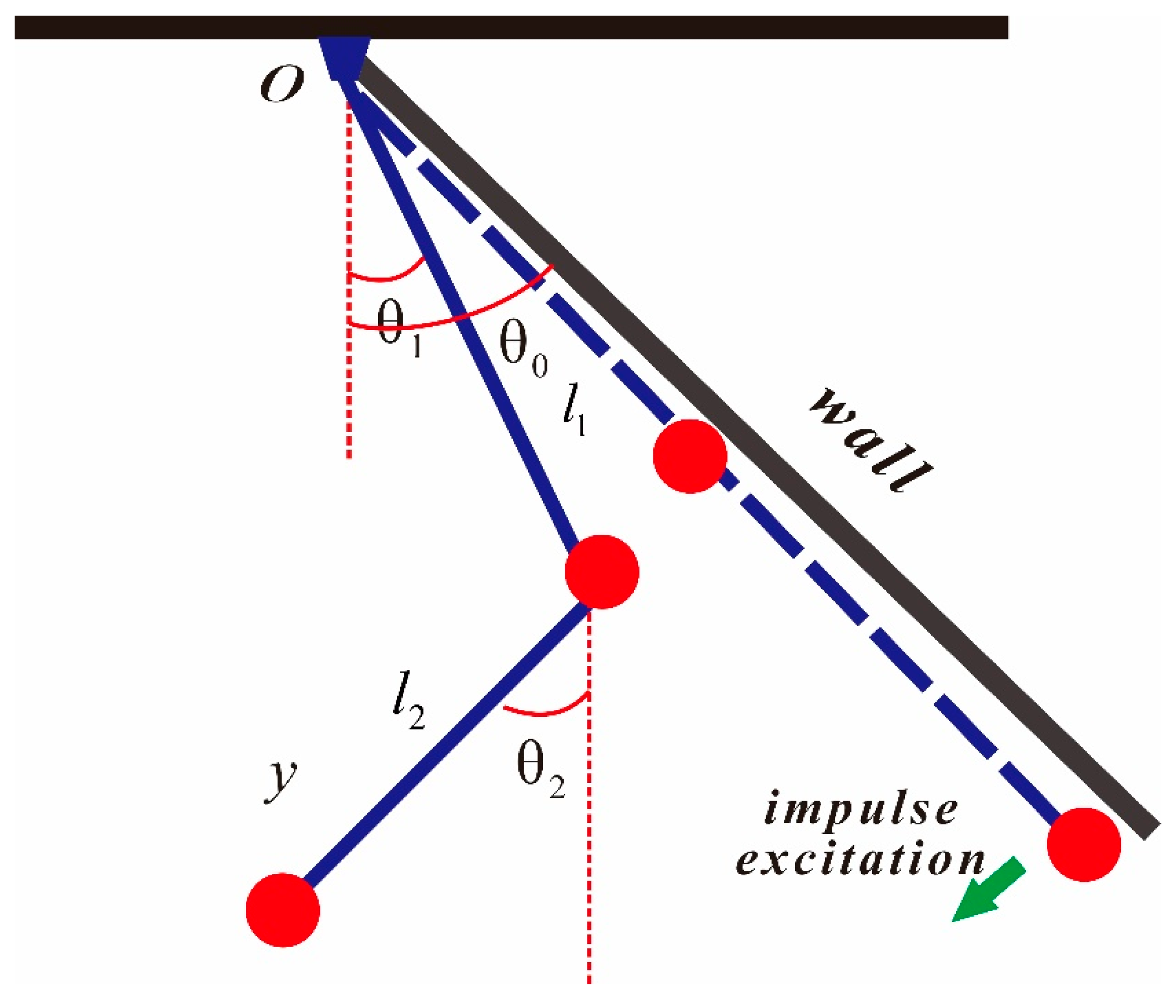
Based on the double pendulum, we constructed a physical model of the non-smooth double pendulum with unilateral rigid constraint as shown in Figure 1. The model consists of a smooth hinged double pendulum with a rigid wall fixed to the base with a horizontal simple harmonic excitation $A\cos (\mathsf{\Omega }t)$. $A,\mathsf{\Omega }$ are the amplitude and frequency of the horizontal simple harmonic excitation. Here, only consider the small angular motion of the two pendulums in the vertical plane, which means ${\theta }_0-{\theta }^{*}\le {\theta }_1\le {\theta }_0$ and ${\theta }_0-{\theta }^{*}\le {\theta }_2\le {\theta }_0$(${\theta }^{*}$ is a smaller positive number). Assume that the angular velocity is positive in the counter clockwise direction.

Where $l_1,l_2;m_1,m_2;c_1,c_2$ are the lengths of the two pendulums, the mass of two pendulums, and the damper of the hinge joint, respectively. Assuming the two pendulums can only swing at a small angle is considered and the elastic collision of the pendulum occurs at the rigid wall ${\theta }_i={\theta }_0,i=1,2$. That is to say, the deformation and time during the pulse excitation are ignored.

When the pendulum collides with the rigid wall, the vector field of the system will have a sudden change in momentum. The phase diagram and time history diagram will be asymmetrical discontinuity, as shown in Figure 2a,b.

In the system, the pendulum angles ${\theta }_1$ and ${\theta }_2$ of the double pendulum are taken as generalized coordinates. According to Lagrange function method, the equation of the system can be obtained

$$\{\begin{array}{l}(m_1+m_2)l_1{}^2{\ddot{\theta }}_1+m_2{l}_1{l}_2{\ddot{\theta }}_2\cos ({\theta }_1-{\theta }_2)+m_2{l}_1{l}_2{\dot{\theta }}_2{}^2\sin ({\theta }_1-{\theta }_2)\\ +(m_1+m_2)g{l}_1\sin {\theta }_1-A{\mathsf{\Omega }}^2(m_1+m_2)l_1\cos (\mathsf{\Omega }t)\cos {\theta }_1=-c_1{\dot{\theta }}_1-c_2({\dot{\theta }}_1-{\dot{\theta }}_2)\\ {\dot{\theta }}_{1+}^{}=-(1-\gamma ){\dot{\theta }}_{1-}^{}{|}_{\theta ={\theta }_0}-\frac{\pi }{2}<{\theta }_1<{\theta }_0\hspace{1em}\\ m_2{l}_2{}^2{\ddot{\theta }}_2+m_2{l}_1{l}_2{\ddot{\theta }}_1\cos ({\theta }_1-{\theta }_2)-m_2{l}_1{l}_2{\dot{\theta }}_1{}^2\sin ({\theta }_1-{\theta }_2)\\ +m_{2}g{l}_1\sin {\theta }_2-A{\mathsf{\Omega }}^2{m}_2{l}_2\cos (\mathsf{\Omega }t)\cos {\theta }_2=c_2({\dot{\theta }}_1-{\dot{\theta }}_2)\hspace{1em}\hspace{1em}\\ {\dot{\theta }}_{2+}^{}=-(1-\gamma ){\dot{\theta }}_{2-}^{}{|}_{\theta ={\theta }_0}-\frac{\pi }{2}<{\theta }_2<{\theta }_0\hspace{1em} \end{array},$$

(1)

where ${\theta }_0\in [0,\frac{\pi }{2}]$, ${\dot{\theta }}_{-}$ and ${\dot{\theta }}_{+}$ represents the angular velocity before and after the impact, respectively. $\gamma (0<\gamma <1)$ is a coefficient of restitution and $(1-\gamma )\in (0,1)$.

Let

$$\begin{array}{l}m=\frac{m_2}{m_1},\xi =\frac{m}{1+m},{\omega }_1^2=\frac{g}{l_1},{\omega }_2^2=\frac{g}{l_2},\mu =\frac{l_1}{l_2},\alpha =\xi {\mu }^{-1},a=\frac{A}{l_1},\omega \tau =\mathsf{\Omega }t,\\ p_1=\frac{c_1}{{\omega }_1{(1+m)}^{\frac{1}{2}}(m_1+m_2)l_1^2},p_2=\frac{c_2}{{\omega }_1{(1+m)}^{\frac{1}{2}}(m_1+m_2)l_1^2},p_3=\frac{c_2}{{\omega }_1{(1+m)}^{\frac{1}{2}}{m}_2{l}_2{}^2}\end{array}$$

(2)

The non-dimensional Equation (1) is written as

$$\{\begin{array}{l}{{\theta }^{″}}_1+\alpha {{\theta }^{″}}_2\cos ({\theta }_1-{\theta }_2)+\alpha {{\theta }^{\prime }}_2{}^2\sin ({\theta }_1-{\theta }_2)+\frac{1}{1+m}\sin {\theta }_1\\ +p_1{{\theta }^{\prime }}_1+p_2({{\theta }^{\prime }}_1-{{\theta }^{\prime }}_2)-a{\omega }^2\cos (\omega \tau )\cos {\theta }_1=0\hspace{1em}\\ {{\theta }^{\prime }}_{1+}^{}=-(1-\gamma ){{\theta }^{\prime }}_{1-}^{}{|}_{\theta ={\theta }_0}\hspace{1em}-\frac{\pi }{2}<{\theta }_1<{\theta }_0\\ {{\theta }^{″}}_2+\mu {{\theta }^{″}}_1\cos ({\theta }_1-{\theta }_2)-\mu {{\theta }^{\prime }}_1{}^2\sin ({\theta }_1-{\theta }_2)+\frac{\mu }{1+m}\sin {\theta }_2\\ +p_3({{\theta }^{\prime }}_2-{{\theta }^{\prime }}_1)-\mu a{\omega }^2\cos (\omega \tau )\cos {\theta }_2=0\hspace{1em}\hspace{1em}\\ {{\theta }^{\prime }}_{2+}^{}=-(1-\gamma ){{\theta }^{\prime }}_{2-}^{}{|}_{\theta ={\theta }_0}-\frac{\pi }{2}<{\theta }_2<{\theta }_0\end{array},$$

(3)

where ${{\theta }^{\prime }}_i$ is a time derivation $\frac{\mathrm{d}{\theta }_i}{\mathrm{d}\tau },i=1,2$.

3. Classification of Periodic Solution

Take $t=0$(${\theta }_1={\theta }_2={\theta }_0$) as the initial time and $T_0=\frac{2n\pi }{\omega }$(${\theta }_1={\theta }_2={\theta }_0$) as the instantaneous of the next collision. This periodic motion, i.e., $[0,T_0]$, is called a one-touch periodic motion.

$s_1$: The top pendulum collides with the rigid constraint:

$${\theta }_1(0)={\theta }_1(T_0)={\theta }_{10},{{\theta }^{\prime }}_1(0)={{\theta }^{\prime }}_1(T_0^{+}),{{\theta }^{\prime }}_1(T_0^{+})=-(1-\gamma ){{\theta }^{\prime }}_1(T_0^{-}).$$

$s_0$: The top pendulum did not collide with the rigid constraint:

$${\theta }_1(0)={\theta }_1(T_0)={\theta }_{10},{{\theta }^{\prime }}_1(0)={{\theta }^{\prime }}_1(T_0)={{\theta }^{\prime }}_{10}.$$

$x_1$: The bottom pendulum collides with the rigid constraint:

$${\theta }_2(0)={\theta }_2(T_0)={\theta }_{20},{{\theta }^{\prime }}_2(0)={{\theta }^{\prime }}_2(T_0^{+}),{{\theta }^{\prime }}_2(T_0^{+})=-(1-\gamma ){{\theta }^{\prime }}_2(T_0^{-}).$$

$x_0$: The bottom pendulum did not collide with the rigid constraint:

$${\theta }_2(0)={\theta }_2(T_0)={\theta }_{20},{{\theta }^{\prime }}_2(0)={{\theta }^{\prime }}_2(T_0)={{\theta }^{\prime }}_{20}.$$

Note that we consider periodic solutions, which implies ${\theta }_{10}={\theta }_{20}={\theta }_0$.

We consider the existence conditions of different types of periodic solutions. The classification of periodic solutions is shown as

Table 1. This classification of periodic solutions.

Type of Solution	Constraint Condition
The first kind of periodic solution	$(s_1,x_1)$
The second kind of periodic solution	$(s_1,x_0)$
The third kind of periodic solution	$(s_0,x_1)$
The forth kind of periodic solution	$(s_0,x_0)$

.

Because of the strong nonlinearity and non-smoothness of the system, it is difficult to find the periodic solution of the original system directly. It is especially difficult to find the periodic analytical solutions of different boundary conditions by selecting reasonable physical parameters and coefficient of restitution of the model. So, considering the small angle oscillation of the manipulator arm (leg) in engineering practice, we study the periodic solution of the small angle motion of the system. Because of non-smoothness, the system is still strongly nonlinear and non-smooth even though it is moving at a small angle. Hence, we will detect the conditions for the existence of parameters of periodic solutions of non-smooth systems and the reference parameters range for the existence of non-smooth periodic solutions can be given.

4. Periodic Solution

In order to facilitate the subsequent analysis, the following approximations

$$\cos ({\theta }_1-{\theta }_2)\approx 1,\sin ({\theta }_1-{\theta }_2)\approx {\theta }_1-{\theta }_2,\sin {\theta }_i\approx {\theta }_i,\cos {\theta }_i\approx 1,i=1,2,{{\theta }^{\prime }}_1{}^2\approx 0,{{\theta }^{\prime }}_2{}^2\approx 0$$

(4)

are given based on the fact that the swings of top and bottom pendulum are enough small during the whole motion process. Substituting (4) into (3), (3) is rewritten as:

$$\{\begin{array}{l}{{\theta }^{″}}_1+\alpha {{\theta }^{″}}_2+\frac{1}{1+m}{\theta }_1+p_1{{\theta }^{\prime }}_1+p_2({{\theta }^{\prime }}_1-{{\theta }^{\prime }}_2)-a{\omega }^2\cos (\omega \tau )=0\\ {{\theta }^{\prime }}_{1+}^{}=-(1-\gamma ){{\theta }^{\prime }}_{1-}^{}{|}_{\theta ={\theta }_0}-\frac{\pi }{2}<{\theta }_1<{\theta }_0\\ {{\theta }^{″}}_2+\mu {{\theta }^{″}}_1+\frac{\mu }{1+m}{\theta }_2+p_3({{\theta }^{\prime }}_2-{{\theta }^{\prime }}_1)-\mu a{\omega }^2\cos (\omega \tau )=0\\ {{\theta }^{\prime }}_{2+}^{}=-(1-\gamma ){{\theta }^{\prime }}_{2-}^{}{|}_{\theta ={\theta }_0}-\frac{\pi }{2}<{\theta }_2<{\theta }_0\end{array},$$

(5)

i.e.,

$$\{\begin{array}{l}{{\theta }^{″}}_1+{\theta }_1-\xi {\theta }_2+k_1{{\theta }^{\prime }}_1-k_2{{\theta }^{\prime }}_2=a{\omega }^2\cos (\omega \tau )\\ {{\theta }^{\prime }}_{1+}^{}=-(1-\gamma ){{\theta }^{\prime }}_{1-}^{}{|}_{\theta ={\theta }_0}-\frac{\pi }{2}<{\theta }_1<{\theta }_0 \\ {{\theta }^{″}}_2-\mu {\theta }_1+\mu {\theta }_2-k_3{{\theta }^{\prime }}_1+k_4{{\theta }^{\prime }}_2=0\\ {{\theta }^{\prime }}_{2+}^{}=-(1-\gamma ){{\theta }^{\prime }}_{2-}^{}{|}_{\theta ={\theta }_0}-\frac{\pi }{2}<{\theta }_2<{\theta }_0\end{array},$$

(6)

where

$$\begin{array}{l}{k}_1=(1+m)(p_1+p_2+\alpha p_3),k_2=(1+m)(p_2+\alpha p_3),\\ k_3=(1+m)(\mu p_1+\mu p_2+p_3),k_4=(1+m)(\mu p_2+p_3).\end{array}$$

Equation (6) can be rewritten as

$$\left(\begin{array}{cc}1& 0\\ 0& 1\end{array}\right)\left(\begin{array}{c}{{\theta }^{″}}_1\\ {{\theta }^{″}}_2\end{array}\right)+\left(\begin{array}{cc}{k}_1& -k_2\\ -k_3& k_4\end{array}\right)\left(\begin{array}{c}{{\theta }^{\prime }}_1\\ {{\theta }^{\prime }}_2\end{array}\right)+\left(\begin{array}{cc}1& -\xi \\ -\mu & \mu \end{array}\right)\left(\begin{array}{c}{\theta }_1\\ {\theta }_2\end{array}\right)=\left(\begin{array}{c}{f}_{10}\cos (\omega \tau )\\ 0\end{array}\right),$$

(7)

$$-\frac{\pi }{2}<{\theta }_i<{\theta }_0,i=1,2,{{\theta }^{\prime }}_{i+}^{}=-(1-\gamma ){{\theta }^{\prime }}_{i-}^{}{|}_{\theta ={\theta }_0}i=1,2.$$

(8)

Clearly, Equation (8) represents collision constraint conditions and impact equation.

Consider the initial conditions

$$\left(\begin{array}{c}{\theta }_1(0)\\ {{\theta }^{\prime }}_1(0)\\ {\theta }_2(0)\\ {{\theta }^{\prime }}_2(0)\end{array}\right)=\left(\begin{array}{c}{\theta }_0\\ {{\theta }^{\prime }}_{10}\\ {\theta }_0\\ {{\theta }^{\prime }}_{20}\end{array}\right)({\theta }_0\ne 0,{{\theta }^{\prime }}_{10}\ge 0,{{\theta }^{\prime }}_{20}\ge 0),$$

(9)

Let ${\omega }_1$ and ${\omega }_2$ be the natural frequencies of system (7). Without collision, they can be written as

$${\omega }_1=\sqrt{\frac{1+\mu +\sqrt{{\left(1+\mu \right)}^2-4\mu (1-\xi )}}{2}},{\omega }_2=\sqrt{\frac{1+\mu -\sqrt{{\left(1+\mu \right)}^2-4\mu (1-\xi )}}{2}}.$$

(10)

Assume that

$$\mathsf{\Phi }=\left(\begin{array}{cc}{\phi }_{11}& {\phi }_{12}\\ {\phi }_{21}& {\phi }_{22}\end{array}\right)=\left(\begin{array}{cc}\frac{1}{\sqrt{1+{(1-{\omega }_1^2)}^2}}& \frac{1}{\sqrt{1+{(1-{\omega }_2^2)}^2}}\\ \frac{1-{\omega }_1^2}{\sqrt{1+{(1-{\omega }_1^2)}^2}}& \frac{1-{\omega }_2^2}{\sqrt{1+{(1-{\omega }_2^2)}^2}}\end{array}\right)$$

(11)

is the regular mode matrix of system (7).

Take

$$X=\mathsf{\Phi }y,$$

(12)

where $X={\left({\theta }_1,{\theta }_2\right)}^T,y={\left(y_1,y_2\right)}^T$. Equation (7) can be decoupled to

$$I\ddot{y}+C\dot{y}+\mathsf{\Lambda }y=F\cos (\omega t),$$

(13)

where

$$I=\left(\begin{array}{cc}1& 0\\ 0& 1\end{array}\right),C=\left(\begin{array}{cc}2\zeta {\omega }_1^2& 0\\ 0& 2\zeta {\omega }_2^2\end{array}\right),\mathsf{\Lambda }=\left(\begin{array}{cc}{\omega }_1^2& 0\\ 0& {\omega }_2^2\end{array}\right),$$

$$F={\left(\begin{array}{cc}{f}_1& f_2\end{array}\right)}^T={\mathsf{\Phi }}^{T}P,P={\left(\begin{array}{cc}{f}_{10}& 0\end{array}\right)}^T.$$

Using the modal superposition method and considering the transformation (12), the solutions of system (7) are obtained as follows

$${\theta }_i(t)={\displaystyle \sum _{j=1}^2{\phi }_{ij}(e^{-{\eta }_{j}t}(a_j\cos ({\omega }_{dj}t)+b_j\sin ({\omega }_{dj}t))+A_j\sin \omega t+B_j\cos \omega t)}$$

(14)

$$\begin{array}{l}{{\theta }^{\prime }}_i(t)={\displaystyle \sum _{j=1}^2{\phi }_{ij}(e^{-{\eta }_{j}t}(b_j{\omega }_{dj}-{\eta }_j{a}_j)\cos ({\omega }_{dj}t)-(a_j{\omega }_{dj}+{\eta }_j{b}_j)\sin ({\omega }_{dj}t))}\\ +A_j\omega \cos (\omega t)-B_j\omega \sin (\omega t))\end{array}$$

(15)

where ${\omega }_{dj}=\sqrt{{\omega }_j^2-{\eta }_j^2}$,${\eta }_j=\zeta {\omega }_j^2,$$a_j,b_j$ is the integral constant determined by the initial condition of system (6), $i=1,2$.

Let $C(t)$ and $D$ are matrices defined as follows

$$C(t)=\left(\begin{array}{cccc}{\phi }_{11}{e}_1{c}_{d1}& {\phi }_{12}{e}_2{c}_{d2}& {\phi }_{11}{e}_1{s}_{d1}& {\phi }_{12}{e}_2{s}_{d2}\\ -{\phi }_{11}{e}_1{g}_{d_1}& -{\phi }_{12}{e}_2{g}_{d_2}& {\phi }_{11}{e}_1{h}_{d_1}& {\phi }_{12}{e}_2{h}_{d_2}\\ {\phi }_{21}{e}_1{c}_{d1}& {\phi }_{22}{e}_2{c}_{d2}& {\phi }_{21}{e}_1{s}_{d1}& {\phi }_{22}{e}_2{s}_{d2}\\ -{\phi }_{21}{e}_1{g}_{d_1}& -{\phi }_{22}{e}_2{g}_{d_2}& {\phi }_{21}{e}_1{h}_{d_1}& {\phi }_{22}{e}_2{h}_{d_2}\end{array}\right),$$

$$D=\left(\begin{array}{cccc}{\phi }_{11}& {\phi }_{12}& 0& 0\\ 0& 0& -{\phi }_{11}& -{\phi }_{12}\\ {\phi }_{21}& {\phi }_{22}& 0& 0\\ 0& 0& -{\phi }_{21}& -{\phi }_{22}\end{array}\right),$$

(14) and (15) can be rewritten as

$$\left(\begin{array}{c}{\theta }_1(t)\\ {{\theta }^{\prime }}_1(t)\\ {\theta }_2(t)\\ {{\theta }^{\prime }}_2(t)\end{array}\right)=C(t)\left(\begin{array}{c}{a}_1\\ a_2\\ b_1\\ b_2\end{array}\right)+D\left(\begin{array}{c}{A}_1\sin \omega t+B_1\cos \omega t\\ A_2\sin \omega t+B_2\cos \omega t\\ \omega (B_1\sin \omega t-A_1\cos \omega t)\\ \omega (B_2\sin \omega t-A_2\cos \omega t)\end{array}\right),$$

(16)

where $c_{d1}=\cos {\omega }_{d1}t,c_{d2}=\cos {\omega }_{d2}t,s_{d1}=\sin {\omega }_{d1}t,s_{d2}=\sin {\omega }_{d2}t,e_1=e^{-{\eta }_{1}t},e_2=e^{-{\eta }_{2}t},$ $g_{d_1}={\eta }_1{c}_{d1}+{\omega }_{d1}{s}_1,g_{d_2}={\eta }_2{c}_2+{\omega }_{d2}{s}_2,h_{d_1}={\omega }_{d1}{c}_1-{\eta }_1{s}_1,h_{d_2}={\omega }_{d2}{c}_2-{\eta }_2{s}_2,$

$$A_j=\frac{{\omega }_j^2-{\omega }^2}{{\left({\omega }_j^2-{\omega }^2\right)}^2+4{\zeta }^2{\omega }_j^4{\omega }^2}{f}_j,j=1,2$$

(17)

$$B_j=\frac{-2\zeta {\omega }_j^2\omega }{{\left({\omega }_j^2-{\omega }^2\right)}^2+4{\zeta }^2{\omega }_j^4{\omega }^2}{f}_j,j=1,2$$

(18)

According to Table 1, considering the first kind of collision periodic solutions, the impact periodic solution should satisfy conditions $s_1$ and $x_1$.

From (9), (16) and $t=0$, we have

$$\left(\begin{array}{c}{\theta }_{10}\\ {{\theta }^{\prime }}_{10}\\ {\theta }_{10}\\ {{\theta }^{\prime }}_{20}\end{array}\right)=C(0)\left(\begin{array}{c}{a}_1\\ a_2\\ b_1\\ b_2\end{array}\right)+D\left(\begin{array}{c}{B}_1\\ B_2\\ -\omega A_1\\ -\omega A_2\end{array}\right)=\left(\begin{array}{c}{\theta }_0\\ {{\theta }^{\prime }}_{10}\\ {\theta }_0\\ {{\theta }^{\prime }}_{20}\end{array}\right),$$

(19)

where

$$C(0)=\left(\begin{array}{cccc}{\phi }_{11}& {\phi }_{12}& 0& 0\\ -{\eta }_1{\phi }_{11}& -{\eta }_2{\phi }_{12}& {\phi }_{11}{\omega }_{d1}& {\phi }_{12}{\omega }_{d2}\\ {\phi }_{21}& {\phi }_{22}& 0& 0\\ -{\eta }_1{\phi }_{21}& -{\eta }_2{\phi }_{22}& {\phi }_{21}{\omega }_{d2}& {\phi }_{22}{\omega }_{d2}\end{array}\right),D=\left(\begin{array}{cccc}{\phi }_{11}& {\phi }_{12}& 0& 0\\ 0& 0& -{\phi }_{11}& -{\phi }_{12}\\ {\phi }_{21}& {\phi }_{22}& 0& 0\\ 0& 0& -{\phi }_{21}& -{\phi }_{22}\end{array}\right).$$

Moreover, ${\theta }_0\ne 0,{{\theta }^{\prime }}_{10}\ge 0,{{\theta }^{\prime }}_{20}\ge 0$ should be satisfied.

So, the integral constant $a_j,b_j(j=1,2)$ should yield

$$\{\begin{array}{l}{\phi }_{11}{a}_1+{\phi }_{12}{a}_2+{\phi }_{11}{B}_1+{\phi }_{12}{B}_2\ne 0\\ {\phi }_{21}{a}_1+{\phi }_{22}{a}_2+{\phi }_{21}{B}_1+{\phi }_{22}{B}_2\ne 0\\ -{\eta }_1{\phi }_{11}{a}_1-{\eta }_2{\phi }_{12}{a}_2+{\phi }_{11}{\omega }_{d1}{b}_1+{\phi }_{12}{\omega }_{d2}{b}_2+\omega {\phi }_{11}{A}_1+\omega {\phi }_{12}{A}_2\ge 0\\ -{\eta }_1{\phi }_{21}{a}_1-{\eta }_2{\phi }_{22}{a}_2+{\phi }_{21}{\omega }_{d1}{b}_1+{\phi }_{22}{\omega }_{d2}{b}_2+\omega {\phi }_{21}{A}_1+\omega {\phi }_{22}{A}_2\ge 0\end{array}.$$

(20)

Note $T_0^{-}$ and $T_0^{+}$ are the moments before and after the collision. Since the collision is instantaneous, there are $T_0=T_0^{-}=T_0^{+}$. Collision condition can be expressed as

$$\left(\begin{array}{c}{\theta }_1(T_0^{+})\\ {{\theta }^{\prime }}_1(T_0^{+})\\ {\theta }_2(T_0^{+})\\ {{\theta }^{\prime }}_2(T_0^{+})\end{array}\right)=\left(\begin{array}{c}{\theta }_1(0)\\ {{\theta }^{\prime }}_1(0)\\ {\theta }_2(0)\\ {{\theta }^{\prime }}_2(0)\end{array}\right)=\left(\begin{array}{c}{\theta }_0\\ {{\theta }^{\prime }}_{10}\\ {\theta }_0\\ {{\theta }^{\prime }}_{20}\end{array}\right)$$

(21)

$$\left(\begin{array}{c}{\theta }_1(T_0^{+})\\ {{\theta }^{\prime }}_1(T_0^{+})\\ {\theta }_2(T_0^{+})\\ {{\theta }^{\prime }}_2(T_0^{+})\end{array}\right)=R_1\left(\begin{array}{c}{\theta }_1(T_0^{-})\\ {{\theta }^{\prime }}_1(T_0^{-})\\ {\theta }_2(T_0^{-})\\ {{\theta }^{\prime }}_2(T_0^{-})\end{array}\right)$$

(22)

where

$$R_1=\left(\begin{array}{cccc}1& 0& 0& 0\\ 0& -(1-\gamma )& 0& 0\\ 0& 0& 1& 0\\ 0& 0& 0& -(1-\gamma )\end{array}\right),R_1{}^{-1}=\left(\begin{array}{cccc}1& 0& 0& 0\\ 0& -\frac{1}{(1-\gamma )}& 0& 0\\ 0& 0& 1& 0\\ 0& 0& 0& -\frac{1}{(1-\gamma )}\end{array}\right).$$

(23)

So, from (21) and (22), we can obtain

$$\left(\begin{array}{c}{\theta }_1(T_0^{-})\\ {{\theta }^{\prime }}_1(T_0^{-})\\ {\theta }_2(T_0^{-})\\ {{\theta }^{\prime }}_2(T_0^{-})\end{array}\right)=R_1{}^{-1}\left(\begin{array}{c}{\theta }_1(T_0^{+})\\ {{\theta }^{\prime }}_1(T_0^{+})\\ {\theta }_2(T_0^{+})\\ {{\theta }^{\prime }}_2(T_0^{+})\end{array}\right)=R_1{}^{-1}\left(\begin{array}{c}{\theta }_0\\ {{\theta }^{\prime }}_{10}\\ {\theta }_0\\ {{\theta }^{\prime }}_{20}\end{array}\right).$$

(24)

Moreover, $R_1$ is called the corresponding collision recovery matrix for the collision conditions $s_1$ and $x_1$.

According to Equation (16),

$$\left(\begin{array}{c}{\theta }_1(T_0^{-})\\ {{\theta }^{\prime }}_1(T_0^{-})\\ {\theta }_2(T_0^{-})\\ {{\theta }^{\prime }}_2(T_0^{-})\end{array}\right)=C(T_0^{-})\left(\begin{array}{c}{a}_1\\ a_2\\ b_1\\ b_2\end{array}\right)+D\left(\begin{array}{c}{A}_1\sin (\omega T_0^{-})+B_1\cos (\omega T_0^{-})\\ A_2\sin (\omega T_0^{-})+B_2\cos (\omega T_0^{-})\\ \omega (B_1\sin (\omega T_0^{-})-A_1\cos (\omega T_0^{-}))\\ \omega (B_2\sin (\omega T_0^{-})-A_2\cos (\omega T_0^{-}))\end{array}\right)$$

(25)

where

$$\begin{array}{c}C(T_0^{-})=\left(\begin{array}{cccc}{\phi }_{11}{e}_1{c}_{d1}& {\phi }_{12}{e}_2{c}_{d2}& {\phi }_{11}{e}_1{s}_{d1}& {\phi }_{12}{e}_2{s}_{d2}\\ -{\phi }_{11}{e}_1{g}_1& -{\phi }_{12}{e}_2{g}_2& {\phi }_{11}{e}_1{h}_1& {\phi }_{12}{e}_2{h}_2\\ {\phi }_{21}{e}_1{c}_{d1}& {\phi }_{22}{e}_2{c}_{d2}& {\phi }_{21}{e}_1{s}_{d1}& {\phi }_{22}{e}_2{s}_{d2}\\ -{\phi }_{21}{e}_1{g}_1& -{\phi }_{22}{e}_2{g}_2& {\phi }_{21}{e}_1{h}_1& {\phi }_{22}{e}_2{h}_2\end{array}\right),\\ g_1={\eta }_1{c}_1+{\omega }_{d1}{s}_1,g_2={\eta }_2{c}_2+{\omega }_{d2}{s}_2,h_1={\omega }_{d1}{c}_1-{\eta }_1{s}_1,h_2={\omega }_{d2}{c}_2-{\eta }_2{s}_2,\\ c_1=\cos (\frac{2n\pi {\omega }_{d1}}{\omega }),\end{array}$$

$$s_1=\sin (\frac{2n\pi {\omega }_{d1}}{\omega }),c_2=\cos (\frac{2n\pi {\omega }_{d2}}{\omega }),s_2=\sin (\frac{2n\pi {\omega }_{d2}}{\omega }),D=\left(\begin{array}{cccc}{\phi }_{11}& {\phi }_{12}& 0& 0\\ 0& 0& -{\phi }_{11}& -{\phi }_{12}\\ {\phi }_{21}& {\phi }_{22}& 0& 0\\ 0& 0& -{\phi }_{21}& -{\phi }_{22}\end{array}\right)$$

From (24) and (25),

$$R_1{}^{-1}\left(\begin{array}{c}{\theta }_0\\ {{\theta }^{\prime }}_{10}\\ {\theta }_0\\ {{\theta }^{\prime }}_{20}\end{array}\right)=C(T_0^{-})\left(\begin{array}{c}{a}_1\\ a_2\\ b_1\\ b_2\end{array}\right)+D\left(\begin{array}{c}{B}_1\\ B_2\\ -\omega A_1\\ -\omega A_2\end{array}\right)$$

(26)

can be known.

From (26),

$$\left(\begin{array}{c}{\theta }_0\\ {{\theta }^{\prime }}_{10}\\ {\theta }_0\\ {{\theta }^{\prime }}_{20}\end{array}\right)=R_{1}C(T_0^{-})\left(\begin{array}{c}{a}_1\\ a_2\\ b_1\\ b_2\end{array}\right)+R_{1}D\left(\begin{array}{c}{B}_1\\ B_2\\ -\omega A_1\\ -\omega A_2\end{array}\right)$$

(27)

can be obtained.

From (19) and (27), we can obtain

$$C(0)\left(\begin{array}{c}{a}_1\\ a_2\\ b_1\\ b_2\end{array}\right)+D\left(\begin{array}{c}{B}_1\\ B_2\\ -\omega A_1\\ -\omega A_2\end{array}\right)=R_{1}C(T_0^{-})\left(\begin{array}{c}{a}_1\\ a_2\\ b_1\\ b_2\end{array}\right)+R_{1}D\left(\begin{array}{c}{B}_1\\ B_2\\ -\omega A_1\\ -\omega A_2\end{array}\right),$$

(28)

i.e.,

$$(C(0)-R_{1}C(T_0^{-}))\left(\begin{array}{c}{a}_1\\ a_2\\ b_1\\ b_2\end{array}\right)=(R_1-E)D\left(\begin{array}{c}{B}_1\\ B_2\\ -\omega A_1\\ -\omega A_2\end{array}\right),$$

(29)

where $A_1,A_2,B_1,B_2$ are the constants determined by the physical parameters of the system. The existence problem of non-smooth periodic solution of system (6) is transformed into the existence of solutions of (20) and (29). In summary, we can draw a conclusion as follows.

Theorem 1.

If the parameters of the collision system (6) satisfy the condition (20) and (29), system (6) has a one-impact periodic motion.

Let

$$\begin{array}{l}{k}_1=1-e_1{c}_1,k_2=1-e_2{c}_2,m_1=e_1{s}_1,m_2=e_2{s}_2,\\ n_1={\eta }_1-(1-\gamma )e_1{g}_1,n_2={\eta }_2-(1-\gamma )e_2{g}_2,\\ p_1={\omega }_{d1}-(1-\gamma )e_1{h}_1,p_2={\omega }_{d2}-(1-\gamma )e_2{h}_2,\\ u_1=\omega (\gamma -2)({\phi }_{11}{A}_1+{\phi }_{12}{A}_2),u_2=\omega (\gamma -2)({\phi }_{21}{A}_1+{\phi }_{22}{A}_2),\end{array}$$

(30)

Equation (29) can be expressed as follows

$$\left(\begin{array}{cccc}{\phi }_{11}{k}_1& {\phi }_{12}{k}_2& -{\phi }_{11}{m}_1& -{\phi }_{12}{m}_2\\ -{\phi }_{11}{n}_1& -{\phi }_{12}{n}_2& {\phi }_{11}{p}_1& {\phi }_{12}{p}_2\\ {\phi }_{21}{k}_1& {\phi }_{22}{k}_2& -{\phi }_{21}{m}_1& -{\phi }_{22}{m}_2\\ -{\phi }_{21}{n}_1& -{\phi }_{22}{n}_2& {\phi }_{21}{p}_1& {\phi }_{22}{p}_2\end{array}\right)\left(\begin{array}{c}{a}_1\\ a_2\\ b_1\\ b_2\end{array}\right)=\left(\begin{array}{c}0\\ u_1\\ 0\\ u_2\end{array}\right).$$

(31)

When

$$k_1\ne 0,k_2\ne 0,k_1{p}_1-m_1{n}_1\ne 0,k_2{p}_2-m_2{n}_2\ne 0,$$

(32)

by constructing an appropriate invertible transformation matrix

$$P=\left(\begin{array}{cccc}\frac{{\phi }_{22}{p}_1}{{\mathrm{{\rm P}}}_1}& \frac{{\phi }_{22}{m}_1}{{\mathrm{{\rm P}}}_1}& \frac{-{\phi }_{12}{p}_1}{{\mathrm{{\rm P}}}_1}& \frac{-{\phi }_{12}{m}_1}{{\mathrm{{\rm P}}}_1}\\ \frac{-{\phi }_{21}{p}_2}{{\mathrm{{\rm P}}}_2}& \frac{-{\phi }_{21}{m}_2}{{\mathrm{{\rm P}}}_2}& \frac{{\phi }_{11}{p}_2}{{\mathrm{{\rm P}}}_2}& \frac{{\phi }_{11}{m}_2}{{\mathrm{{\rm P}}}_2}\\ \frac{{\phi }_{22}{n}_1}{{\mathrm{{\rm P}}}_1}& \frac{{\phi }_{22}{k}_1}{{\mathrm{{\rm P}}}_1}& \frac{-{\phi }_{12}{n}_1}{{\mathrm{{\rm P}}}_1}& \frac{-{\phi }_{12}{k}_1}{{\mathrm{{\rm P}}}_1}\\ \frac{-{\phi }_{21}{n}_1}{{\mathrm{{\rm P}}}_1}& \frac{-{\phi }_{21}{k}_2}{{\mathrm{{\rm P}}}_1}& \frac{{\phi }_{11}{n}_2}{{\mathrm{{\rm P}}}_1}& \frac{{\phi }_{11}{k}_2}{{\mathrm{{\rm P}}}_1}\end{array}\right),$$

Equation (31) can be taken as

$$\left(\begin{array}{cccc}1& 0& 0& 0\\ 0& 1& 0& 0\\ 0& 0& 1& 0\\ 0& 0& 0& 1\end{array}\right)\left(\begin{array}{c}{a}_1\\ a_2\\ b_1\\ b_2\end{array}\right)=\left(\begin{array}{c}\frac{m_1({\phi }_{22}{u}_1-{\phi }_{12}{u}_2)}{P_1}\\ \frac{m_2({\phi }_{11}{u}_2-{\phi }_{12}{u}_1)}{P_2}\\ \frac{k_1({\phi }_{22}{u}_1-{\phi }_{12}{u}_2)}{P_1}\\ \frac{k_1({\phi }_{11}{u}_2-{\phi }_{12}{u}_1)}{P_2}\end{array}\right),$$

(33)

where $P_1=({\phi }_{11}{\phi }_{22}-{\phi }_{12}{\phi }_{21})(k_1{p}_1-m_1{n}_1),P_2=({\phi }_{11}{\phi }_{22}-{\phi }_{12}{\phi }_{21})(k_2{p}_2-m_2{n}_2)$.

If the physical parameters and the collision recovery coefficient of system (6) are given, the unique integral constant $a_j,b_j(j=1,2)$ can be calculated from (32) as follows

$$a_1=\frac{m_1({\phi }_{22}{u}_1-{\phi }_{12}{u}_2)}{({\phi }_{11}{\phi }_{22}-{\phi }_{12}{\phi }_{21})(k_1{p}_1-m_1{n}_1)},a_2=\frac{m_2({\phi }_{11}{u}_2-{\phi }_{12}{u}_1)}{({\phi }_{11}{\phi }_{22}-{\phi }_{12}{\phi }_{21})(k_2{p}_2-m_2{n}_2)}$$

(34)

$$b_1=\frac{k_1({\phi }_{22}{u}_1-{\phi }_{12}{u}_2)}{({\phi }_{11}{\phi }_{22}-{\phi }_{12}{\phi }_{21})(k_1{p}_1-m_1{n}_1)},b_2=\frac{k_1({\phi }_{11}{u}_2-{\phi }_{12}{u}_1)}{({\phi }_{11}{\phi }_{22}-{\phi }_{12}{\phi }_{21})(k_2{p}_2-m_2{n}_2)}$$

(35)

Therefore, from (14), (20), (34), and (35), the first kind of collision periodic solution of system (6) is obtained

$$\begin{array}{l}{\theta }_i(t)={\displaystyle \sum _{j=1}^2{\phi }_{ij}(e^{-{\eta }_{j}t}(a_j\cos ({\omega }_{dj}t)+b_j\sin ({\omega }_{dj}t))+A_j\sin \omega t+B_j\cos \omega t)}\\ \hspace{1em}(i=1,2)(t=0\hspace{0.17em}\mathrm{mod}\hspace{0.17em}2n\pi /\omega )\end{array}$$

(36)

Moreover, when $k_1\ne 0,k_2\ne 0,k_1{p}_1-m_1{n}_1\ne 0,k_2{p}_2-m_2{n}_2\ne 0$ are not held, (29) has an infinite number of solutions or no solutions, which leads to many periodic or no periodic solutions in the original system (6).

For example, if $k_1\ne 0,k_2\ne 0,k_1{p}_1-m_1{n}_1\ne 0$, $k_2{p}_2-m_2{n}_2=0$, (31) is equivalent to

$$\left(\begin{array}{cccc}{\phi }_{11}{k}_1& {\phi }_{12}{k}_2& -{\phi }_{11}{m}_1& -{\phi }_{12}{m}_2\\ 0& 0& {\phi }_{11}(p_1-\frac{m_1}{k_1}{n}_2)& {\phi }_{12}(p_2-\frac{m_2}{k_2}{n}_2)\\ 0& 1& 0& \frac{-m_2}{k_2}\\ 0& 0& 0& p_2-\frac{m_2}{k_2}{n}_2\end{array}\right)\left(\begin{array}{c}{a}_1\\ a_2\\ b_1\\ b_2\end{array}\right)=\left(\begin{array}{c}0\\ u_1\\ 0\\ \frac{{\phi }_{11}{u}_2-{\phi }_{21}{u}_1}{{\phi }_{11}{\phi }_{22}-{\phi }_{12}{\phi }_{21}}\end{array}\right).$$

(37)

When ${\phi }_{11}{u}_2-{\phi }_{21}{u}_1\ne 0$ or $u_1\ne 0$ is true, Equation (37) has no solution. Hence, system (6) has no collision periodic solution.

Note 1 Conditions (20) and (32) are sufficient and unnecessary conditions for system (6) with the first kind of collision periodic solution.

Note 2 The collision recovery matrices $R_2,R_3,R_4$ of the second type, the third type, and the fourth type of periodic solutions can be shown as

$$R_2=\left(\begin{array}{cccc}1& 0& 0& 0\\ 0& -(1-\gamma )& 0& 0\\ 0& 0& 1& 0\\ 0& 0& 0& 1\end{array}\right),R_3=\left(\begin{array}{cccc}1& 0& 0& 0\\ 0& 1& 0& 0\\ 0& 0& 1& 0\\ 0& 0& 0& -(1-\gamma )\end{array}\right),R_4=\left(\begin{array}{cccc}1& 0& 0& 0\\ 0& 1& 0& 0\\ 0& 0& 1& 0\\ 0& 0& 0& 1\end{array}\right).$$

In order to get the second type, the third type and the fourth type of periodic solutions, $R_1$ can be replaced by $R_i,i=2,3,4$ in Equation (28), we have

$$(C(0)-R_{i}C(T_0^{-}))\left(\begin{array}{c}{a}_1\\ a_2\\ b_1\\ b_2\end{array}\right)=(R_i-E)D\left(\begin{array}{c}{B}_1\\ B_2\\ -\omega A_1\\ -\omega A_2\end{array}\right),i=2,3,4$$

(38)

Clearly, for specific matrices, invertible transformation matrices can be constructed. Similar methods can be used to obtain the existence conditions and analytical expressions of periodic solutions.

5. Numerical Simulation

In order to verify the results of theoretical analysis, the suitable physical parameters and coefficient of restitution are selected to solve the periodic solutions according to (20) and (32). From (17), (18), and (20), we know $A_2=0,B_2=0$ and

$$\{\begin{array}{l}{\phi }_{11}{a}_1+{\phi }_{12}{a}_2+{\phi }_{11}{B}_1\ne 0\\ {\phi }_{21}{a}_1+{\phi }_{22}{a}_2+{\phi }_{21}{B}_1\ne 0\\ -{\eta }_1{\phi }_{11}{a}_1-{\eta }_2{\phi }_{12}{a}_2+{\phi }_{11}{\omega }_{d1}{b}_1+{\phi }_{12}{\omega }_{d2}{b}_2+\omega {\phi }_{11}{A}_1\ge 0\\ -{\eta }_1{\phi }_{21}{a}_1-{\eta }_2{\phi }_{22}{a}_2+{\phi }_{21}{\omega }_{d1}{b}_1+{\phi }_{22}{\omega }_{d2}{b}_2+\omega {\phi }_{21}{A}_1\ge 0\end{array}.$$

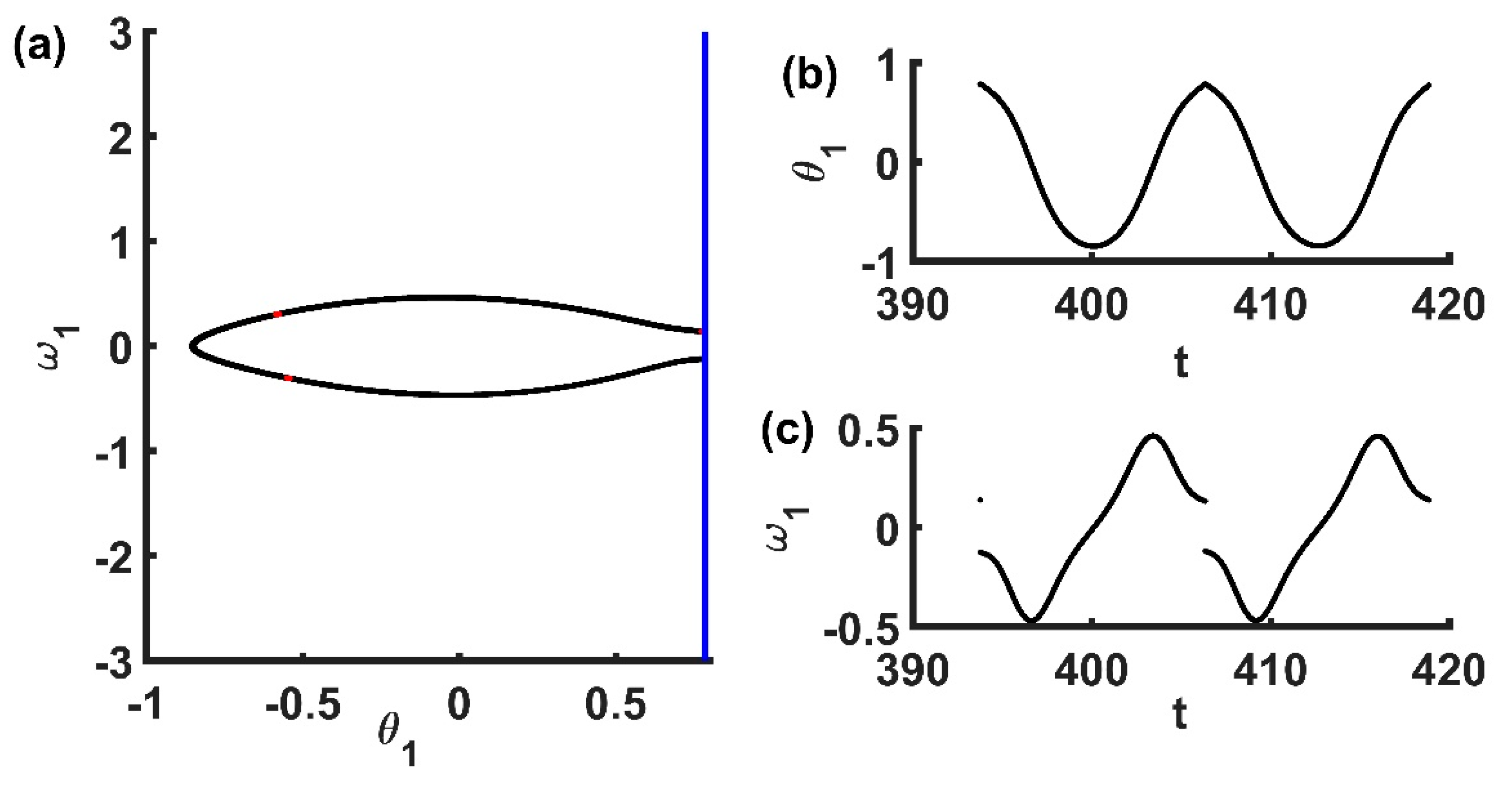
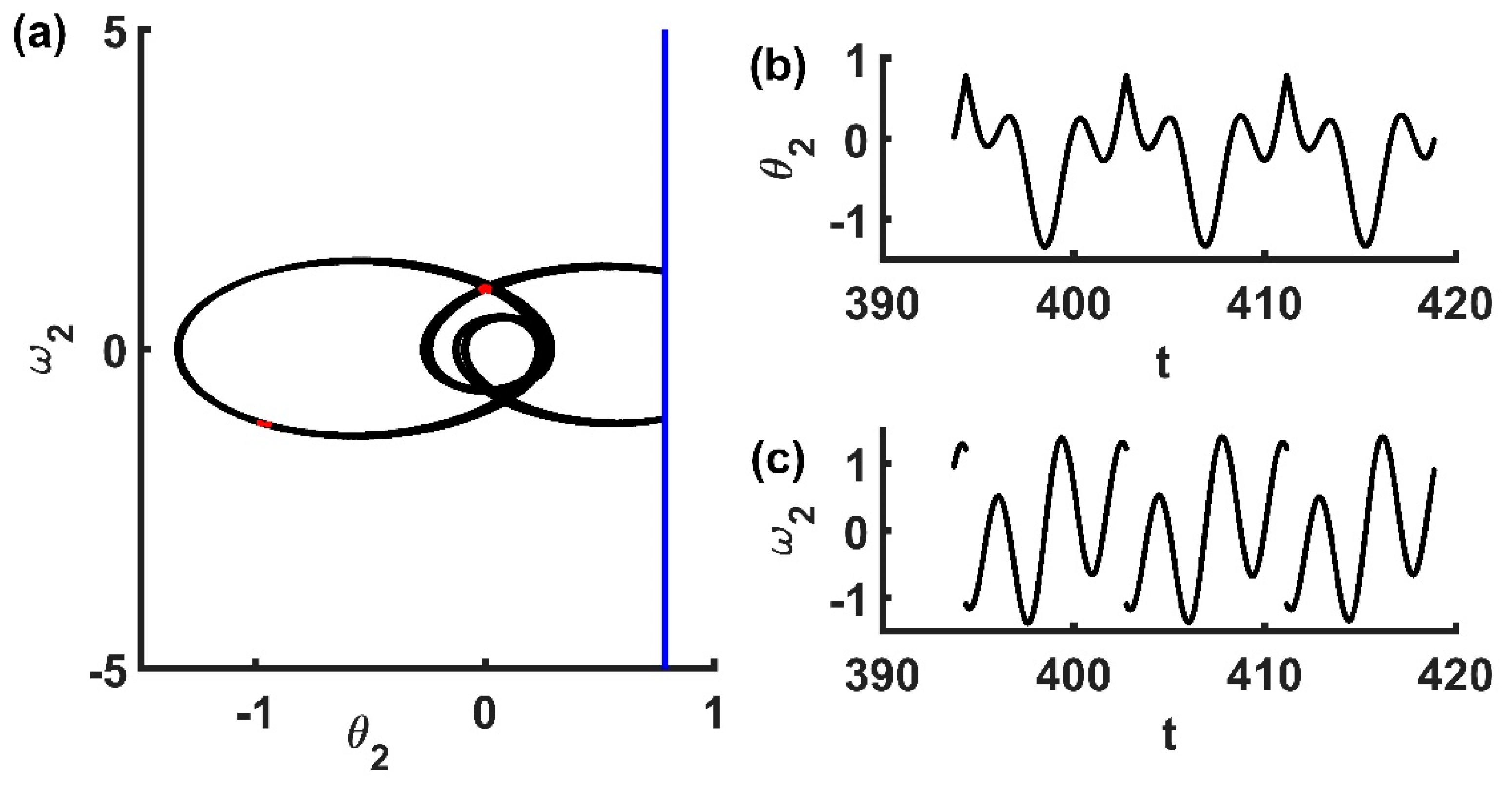
Let $m=3,\mu =3.24,\xi =0.75,\omega =1.5,f_{10}=0.162,\gamma =0.1$, from (20), (30), (31), and (32), the corresponding parameter values are calculated. The phase diagram and Poincare section of the periodic 3 motion of the upper (lower) pendulum of system (6) are shown in Figure 3 and Figure 4. The blue solid line on the right side of the phase diagram is the displacement of the collision point. The red phase point is the projection of the Poincare section on the phase diagram. As can be seen in Figure 3 and Figure 4, the phase diagram and the velocity at the collision point have a momentary jump, indicating that upper (lower) pendulum and the rigid wall collided.

When the parameter value is $m=1,\mu =3.24,\xi =0.5,\omega =1.5,f_{10}=0.22,\gamma =0.1$, from (37) and $R_2$, $a_j,b_j(j=1,2)$ can be obtained. Hence, we get the second kind of collision periodic solution. The phase diagram and Poincare section of the periodic 2 motion of the upper pendulum are shown in Figure 5a and Figure 6a. As can be seen in Figure 5a,c, the phase diagram and the velocity at the collision point have a momentary jump, indicating that upper pendulum and the rigid wall collided. But in Figure 6a, there is a small gap between the phase diagram curve and the blue solid line, which indicates that the upper pendulum does not collide with the right wall. As can be seen from Figure 6c, the velocity diagram is continuous, which further confirms the fact that the lower pendulum does not collide.

When the parameter value is $m=1,\mu =3.2,\xi =0.5,\omega =1.5,f_{10}=0.1,\gamma =0.1$, from (37) and $R_3$, a_j, b_j(j = 1, 2) can be obtained. Hence, we can detect the third kind of collision periodic solution. The phase diagram and Poincare section of the periodic 2 motion are shown in Figure 7a and Figure 8a. As can be seen in Figure 7a, there is a big gap between the phase diagram curve and the blue solid line, indicating that the upper pendulum does not collide with the right wall and the velocity diagram further confirms the fact in Figure 7c. In Figure 8a,c, the phase diagram and the velocity at the collision point have a momentary jump, showing that lower pendulum and the rigid baffle collided with the right wall.

The simulation results show that the collision periodic solution of the system can be found based on the condition of the existence of the collision analytical periodic solution, which provides a theoretical method for studying the periodic solution of the non-smooth system. The case of collision with left wall can be discussed similarly. Due to the complex type of periodic solution, further analysis will be conducted for the case of bilateral constraint, which could be carried out in a separate paper.

6. Conclusions

A kind of asymmetry system has been constructed by use of the non-smooth unilateral rigid constrained double pendulum, which is subjected to harmonic excitation. Using the mode superposition method and matrix theory, the existence conditions of periodic solutions and the expressions of periodic analytical solutions were deduced for small angle vibration of the system. The numerical simulation showed that this method can predict the existence of periodic solutions of collisions. From the previous calculation, it can be seen that the integral constants and existence conditions of three kinds of periodic solutions of collisions can be calculated by introducing matrix tools. This method provided a matrix computing tool for solving the periodic solutions of high-dimensional non-smooth systems, aiming at multi-point collisions. As long as the appropriate collision recovery matrix was found, the calculation process was similar, which provided a mechanized calculation for simplifying the manipulator into several degrees of freedom problems in the research and design of the manipulator. Thus, a method for the fault research of the fine manipulator was provided to facilitate the engineers to use this method to find the periodic solution of the high-dimensional non-smooth system.

References

- Guan, T.M.; Li, N.; Xuan, L.; Wang, M.L. Kinematics Simulation Analysis of Shoulder Joint of New Bionic Robot Arm. J. Dalian Jiaotong Univ. 2018, 39, 65–70. [Google Scholar]
- Yang, Q.Z.; Cao, D.F.; Zhao, J.H. Analysis on State of the Art of Upper Limb Rehabilitation Robots. Robot 2013, 35, 631–640. [Google Scholar] [CrossRef]
- Hong, Z.R. Design Analysis of Mechanism Structure of Bionic Robotic Arm. J. Lanzhou Petrochem. Polytech. 2017, 17, 1–4. [Google Scholar]
- Qian, Z.J.; Zhang, D.G.; Jin, C.Q. A regularized approach for frictional impact dynamics of flexible multi-link manipulator arms considering the dynamic stiffening effect. Multibody Syst. Dyn. 2018, 43, 229–255. [Google Scholar] [CrossRef]
- Kumar, R.; Gupta, S.; Ali, S.F. Energy harvesting from chaos in base excited double pendulum. Mech. Syst. Signal Process. 2019, 124, 49–64. [Google Scholar] [CrossRef]
- Wojna, M.; Wijata, A.; Wasilewski, G.; Awrejcewicz, J. Numerical and experimental study of a double physical pendulum with magnetic interaction. J. Sound Vib. 2018, 430, 214–230. [Google Scholar] [CrossRef]
- Izadgoshasb, I.; Lim, Y.Y.; Tang, L.; Padilla, R.V.; Tang, Z.S.; Sedighi, M.; Sedighi, M. Improving efficiency of piezoelectric based energy harvesting from human motions using double pendulum system. Energy Convers. Manag. 2019, 184, 559–570. [Google Scholar] [CrossRef]
- Battelli, F.; Feckan, M. Nonsmooth homoclinic orbits, Melnikov functions and chaos in discontinuous systems. J. Phys. D 2012, 241, 1962–1975. [Google Scholar] [CrossRef]
- Tian, R.L.; Zhao, Z.J.; Yang, X.W.; Zhou, Y.F. Subharmonic bifurcation for non-smooth oscillator. Int. J. Bifurc. Chaos 2017, 27, 17501631. [Google Scholar] [CrossRef]
- Tian, R.L.; Zhou, Y.F.; Wang, Y.Z.; Feng, W.J.; Yang, X.W. Chaotic threshold for non-smooth system with multiple impulse effect. Nonlinear Dyn. 2016, 85, 1849–1863. [Google Scholar] [CrossRef]
- Tian, R.L.; Zhou, Y.F.; Zhang, B.L.; Yang, X.W. Chaotic threshold for a class of impulsive differential system. Nonlinear Dyn. 2016, 83, 2229–2240. [Google Scholar] [CrossRef]
- Bi, Q.S.; Chen, Y.S. Bifurcation Analysis of a Double Pendulum With Internal Resonance. Appl. Math. Mech. 2000, 21, 226–234. [Google Scholar]
- Han, W.; Hu, H.Y.; Jin, D.P.; Hou, Z.Q. The oblique-impact vibration of a double compound pendulum with the end displacement limit. J. Dyn. Control 2004, 2, 24–30. [Google Scholar]
- Han, W.; Hu, H.Y.; Jin, D.P. Oblique impact analysis of two-degree-of-freedom vibration systems. J. Mech. 2003, 35, 723–729. [Google Scholar]
- Zhu, X.F.; Cao, X.X. Flutter motion and transition law of two-degree-of-freedom elastic collision system. J. Lanzhou Jiaotong Univ. 2014, 33, 191–195. [Google Scholar]
- Hu, H.Y. Numerical analysis of periodic response of high-dimensional non-smooth dynamic systems. Acta Solid Mech. Sin. 1994, 15, 135–145. [Google Scholar]
- Li, Q.H.; Lu, Q.S. Analysis to motions of a two-degree-of-freedom vibro-impact system. Acts Mech. Sin. 2001, 33, 776–786. [Google Scholar]
- Jin, D.P.; Hu, H.Y. Vibro-impacts and their typical behaviors of mechanical systems. Adv. Mech. 1999, 29, 155–164. [Google Scholar]
- Luo, G.W.; Chu, Y.D.; Gou, X.F. Quasi-periodic impact motions and routes to chaos of an impact system with two singer-degree–freedom oscillators. J. Mech. Strength 2005, 27, 445–451. [Google Scholar]
- Luo, G.W.; Xie, J.H.; Sun, X.F. Periodic motions and stability of a two-degree-of-freedom vibro-impact system. J. Lanzhou Railw. Inst. 1999, 18, 47–54. [Google Scholar]
- Cao, D.Q.; Shu, Z.Z. Periodic motions and robust stability of the multi-degree-of-freedom systems with clearances. Acts Mech. Sin. 1997, 29, 74–83. [Google Scholar]
Figure 1.
Collision double pendulum model.
Figure 2.
Phase diagram and time-velocity diagram.
Figure 3.
The first kind of collision periodic solutions: (a) Phase diagram and Poincare section of periodic 3 motion of upper pendulum; (b) Time-displacement diagram of the upper pendulum; (c) Time-velocity diagram of upper pendulum.
Figure 4.
The first kind of collision periodic solution: (a) Phase diagram and Poincare section of periodic 3 motion of lower pendulum; (b) The time-displacement diagram of the lower pendulum; (c) The time-velocity diagram of the lower pendulum.
Figure 5.
The second kind of collision periodic solutions: (a) Phase diagram and Poincare section of periodic 2 motion of upper pendulum; (b) Time-displacement diagram of the upper pendulum; (c) Time-velocity diagram of upper pendulum.
Figure 6.
The second kind of collision periodic solution: (a) phase diagram and Poincare section of periodic 2 motion of lower pendulum; (b) the time-displacement diagram of the lower pendulum; (c) the time-velocity diagram of the lower pendulum.
Figure 7.
The third kind of collision periodic solutions: (a) Phase diagram and Poincare section of periodic 2 motion of upper pendulum; (b) Time-displacement diagram of the upper pendulum; (c) Time-velocity diagram of upper pendulum.
Figure 8.
The third kind of collision periodic solution: (a) Phase diagram and Poincare section of periodic 2 motion of lower pendulum; (b) The time-displacement diagram of the lower pendulum; (c) The time-velocity diagram of the lower pendulum.