Multiple Slip Effects on Magnetohydrodynamic Axisymmetric Buoyant Nanofluid Flow above a Stretching Sheet with Radiation and Chemical Reaction


Department of Applied Mathematics, School of Science, Northwestern Polytechnical University, Dongxiang Road, Chang’an District, Xi’an 710129, China
*
Author to whom correspondence should be addressed.
Symmetry 2019, 11(9), 1171; https://doi.org/10.3390/sym11091171
Submission received: 25 July 2019
/
Revised: 4 September 2019
/
Accepted: 9 September 2019
/
Published: 16 September 2019
(This article belongs to the Special Issue Future and Prospects in Non-Newtonian and Nanofluids)
Abstract
:The present article investigates the effect of multiple slips on axisymmetric magnetohydrodynamics (MHD) buoyant nano-fluid flow over a stretching sheet with radiation and chemical effect. The non-linear partial differential equations were transformed to a non-linear control equation using an appropriate similarity transformation. The governing equations were solved through the finite element method. The influence of physical parameters such as multiple slips, magnetic, thermal radiation, Prandtl number, stretching, Brownian motion, thermophoresis, Schmidt number, Lewis number and chemical reaction on the radial velocity, temperature, solutal concentration and nano-fluid volume fraction profile were investigated. We noted that the boundary layers increases in the presence of multiple slip effects whereas, the effect of thermal slip on Nusselt number increases with the increasing values of magnetic and thermal radiation. To verify the convergence of the numerical solution, the computations were made by reducing the mesh size. Finally, our results are parallel to previous scholarly contributions.
1. Introduction
The study of the hydromagnetics flow of non-Newtonian fluids related to nano-particles has attracted many mathematicians, physician, engineers and modelers due to numerous significant applications. These applications spread through a wide range including neural-electronic interfaces and protein engineering, solar systems, nuclear reactors, cooling systems and so forth. As a result, nano-fluids have been examined both hypothetically and experimentally to attain higher degree characteristics of heat transfer in base fluids. Studies have also focused on improved energy efficiency in an assortment of thermal exchange system for various mechanical, physics and engineering applications. These novel kinds of fluids have attracted numerous researchers in view of its improved thermal features. Compared with basic fluids such as water and oil, nano-fluids possess higher thermal conductivity and convection heat transfer properties. Choi and Eastman [1] empirically established that adding a small amount of these particles would significantly improve their effective thermal conductivity. Buongiorno [2] in his non-homogenous equilibrium model reveals that the abnormal increase in the thermal conductivity occurs due to the presence of Brownian motion and thermophoretic diffusion of nanoparticles. A wide range of current and future applications of nano-fluids are prescribed [3,4,5,6,7,8]. Nield and Kuznetsov [9] used the Buongiorno model to study the nano-fluids with respect to free convection flow problem in the permeable medium. Similarly Salleh et al. [10] conducted numerical analysis of the boundary layer heat flow adjacent to a thin needle in the nano-fluid in the presence of heat source and chemical reaction.
Kuznetsov and Nield [11] analyzed boundary layer flow through a plate and later through a porous medium [12]. Likewise, the flow of nano-fluids on a moving plate in uniform free flow is studied by Bachok et al. [13].
The effect of magnetic field on free convection heat transfer of nano-fluid in sinusoidal wall channel is studied by Rashidi et al. [14]. Numerical study on the flow of nano-fluids in rotating systems with permeable films is carried out by Sheikholeslami et al. [15]. Hatami et al. [16] analyzed nano-fluid flow in axisymmetric porous channels with expansion or shrinkage wall.
Magnetohydrodynamics plays a key role in the field of engineering, agriculture and metal processing. The application of mixed convection problem under the influence of the magnetic field in geophysics and astrophysics has attracted the attention of many researchers. Soundalgekar et al. [17] studied the free convection effect of vertical plates with transverse magnetic fields on Stokes problem, while Elbasheshy [18] studied the problems of MHD heat and mass transfer and the role of vertical plates along with the buoyancy effect of heat and species diffusion. In the MHD flow, the inductive current in the fluid creates a force that changes the flow field. Mohanty et al. [19] studied the reaction of the chemical to MHD fluid with heat generation/absorption on the stretching sheet. In another study, M. Ramzan et al. [20] examined the effects of MHD, Joule heating and thermal radiation on an incompressible Jeffrey nano-fluid flow over a linearly stretched surface. MHD and heat transfer flow on a vertical stretching sheet with heat sink or source effect was studied by M. Alfari et al. [21]. Steady two-dimensional laminar incompressible MHD flow over an exponentially shrinking sheet with the effects of slip conditions and viscous dissipation was examined by Ali Lund et al. [8]. Najib et al. [22] examined the stagnation point flow and mass transfer with chemical reaction through stretch/shrink cylinder. The heat and mass transfer flow of MHD micro-polar fluid in the presence of heat sources was investigated by Mishra et al. [23].
Thermal system performance using common base fluids is relatively poor. One way to improve the performance of these systems is to suspend metal nano-particles in the base fluid. Thermal radiation for heat transfer and mass transfer on tensile surfaces plays an important role because of its numerous applications in engineering and physics fields such as satellites, solar energy, geophysics, geophysics, spacecraft and fossil fuels combustion. We know that concentrations and temperature gradients describe mass and energy flux. These effects have significant role in density difference flow. It is of great help to manufacture, pollute and discover drugs of optical fibers and others. Zaimi [24] sought the influence of heat transfer on the nano-fluid flow by means of permeable stretching/shrinking sheet. Ahmed et al. [25] presented the unsteady boundary layer flow and heat transfer of power-law fluid model over a radially stretching sheet. Heat transfer of viscous fluid over a non-linear radially stretching sheet was studied by Azeem et al. [26]. Ilyas Khan et al. [27] introduced a mathematical model of a convection flow of MHD nano-fluid in a channel embedded in a porous medium. The influence of the external magnetic field and thermal radiation on heat transfer intensification of nano-fluid in a porous curved enclosure is simulated by M. Sheikholeslami et al. [5]. Steady 2-D MHD free convective boundary-layer flows of an electrically conducting nano-fluid over a non-linear stretching sheet, taking into account the chemical reaction and heat source/sink, was investigated by D. Makinde et al. [28]. Multiple Slip Effects on MHD Unsteady Flow Heat and Mass transfer impinging on permeable stretching sheet with radiation is studied by Fazle and Stanford Shateyi [29]. Chemical reaction effect of an axisymmetric flow over a radially stretching sheet was considered by B. Nayak [30].
To the author’s best knowledge, no previous studies have thus far examined the multiple slips on hydromagnetics axisymmetric nano-fluid steady flow, heat and mass transfer influenced by radiation, buoyancy and chemical effect in a permeable frame of reference. We provide numerical solutions for some special cases, while the physical interpretation for the various parameters have been explained with the help of graphs. The current study investigates the analysis of mass and heat transfer in the axisymmetric MHD nano-fluid flow over a stretching sheet in the presence of multiple slip conditions with buoyancy effect, chemical reaction and thermal radiation. The governing partial differential equations of the model are converted to ordinary differential equations ODE through proper similarity transformations. The ODE’s are then solved through finite element method. The numerical results of radial velocity distribution, temperature profile, solutal concentration and nano-fluid volume fraction with different physical parametric values are discussed graphically. The present results are compared with those of published papers [31,32,33] and found a good agreement.
2. Mathematical Formulation
We consider the steady axisymmetric MHD flow of an electrically conducting incompressible viscous flow immersed in nano-fluid over a stretching sheet. The geometry of the problem is illustrated in Figure 1. The flow of conductive fluids is caused by the sheet stretching in the direction, where is a dimensional constant. It is considered that there is no nanoparticle flux across the wall and the surface is stretching along z-direction. Furthermore, it is assumed that , and denotes the stretching sheet temperature, solute concentration and the nano-particle fraction at the sheet respectively. At the infinity the , and are the ambient temperature, ambient solute concentration and ambient nano-particle volume fraction, respectively. In the current study, summarizes the strength of magnetic field, where is a uniform magnetic field strength. The magnetic field acts along normal to the sheet in the positive z-direction. When the magnetic field is varying in the radial direction, it also vary in the vertical direction, since the divergence of B should be zero, that is, . Under the boundary layer approximation, the equations of mass conservation, linear momentum conservation, energy conservation and nano-particle volume fraction (see References [30,34,35,36]) can be obtained as:
where u and w are supposed to be the velocity components along r and z respectively, , and are the kinetic viscosity, electric conductivity and viscosity of fluid, respectively. , , , , are the Brownian diffusion, thermophoretic diffusion, the solutal and chemical reaction, respectively.
The quantity is the relative heat flux. Applying the Rosseland approximation [37], can be defined as:
where and are the Stefan-Boltzmann constant and the mean absorbtion coefficient, respectively. If the variation in temperature across the flow is small, maybe expended using Tayler series at a free stream temperature after neglecting higher-order terms as
Using Equations (7) and (8), we get
To simplify the mass equation, the chemical reaction must be constant. This constraint holds if has the following form [38]:
where is constant and is the stretching constant. The required physical boundary conditions of the above governing Equations are as follows [39]:
where is the thermal slip, is the temperature slip factor, is the solutal slip, is the solutal concentration slip factor, is the slip velocity of the nanoparticle, is the nanoparticle concentration slip factor, is the variable surface concentration, is a constant, n is power-law exponent signifies the change of amount of solute in –direction.
In order to solve Equations (1)–(6), we introduce the following similarity transformations (see References [30,34]):
In view of the similarity transformation equation, the partial nonlinear differential Equations (1)–(6) transform into the following system of nonlinear ODEs:
and the transformed boundary conditions of Equation (10) are:
The primes shows the differentiation with respect to . The parameters in Equations (12)–(17) are defined as: , , , , , , , are magnetic, Prandtl number, Brownian, thermophoresis, Schmidt number, Lewis number, thermal radiation and chemical reaction parameter, respectively. , , are the buoyancy parameters. , , and are the hydrodynamic slip, thermal slip, solutal slip and nano-fluid slip, respectively.
3. Finite Element Method Solutions
We applied the finite element method to solve nonlinear differential Equations (12)–(17), with the boundary conditions (12). Finite element method is extremely efficient and was applied to solve different problems in fluid mechanics, heat transfer, chemical processing, solid mechanics and other fields also (see References [40,41,42]). In order to find numerical solutions, we consider
substitute Equation (13) in to Equation (8)–(11) the system reduce to:
with following reduce boundary condition
For the computation purposes, the at ∞ is chosen large enough, therefore the numerical solution depicts no perceptible variation for larger than . Subject to the boundary condition the has been fixed at .
3.1. Variational Formulations
The variational form associated with Equations (13)–(18) over a linear element is given by
where and are arbitrary shape function or trial function.
3.2. Finite Element Formulations
The Equation of finite element model is obtained by replacing finite element approximation of the following form in the Equations (19)–(23).
with , where the shape function for a line element are given by
The finite element method model equations are, therefore given by
where and (m, n = 1, 2, 3, 4, 5) are defined as
and
where and are considered to be known. After assembling all the element equations the resulting system of equations obtained are nonlinear, therefore an iterative scheme is used in the solution. The system is linearized by incorporating the function , , and known at a lower iteration level. Computations for the functions are carried out for high level. This process is repeated till the desired accuracy of 0.00005 is obtained.
4. Results and Discussion
Research goal of the current study was to identify the role of mass, heat transfer, chemical reaction and thermal radiation in the axisymmetric MHD boundary layer flow of nano-fluid in the presence of multiple slip effects over a stretching sheet. The finite element method was used to solve the control model equations numerically. In this part, we discuss the results of velocity, temperature, solute concentration and the distribution of the volume fraction of nano-fluid by the proposed numerical scheme. We describe the effect of above profiles on the various dimensionless parametric values such as thermal radiation , magnetic M, Prandtl number , stretching parameter n, Brownian motion parameter , buoyancy parameters , thermophoresis , Schmidt number , Lewis number and chemical reaction parameters in the presence of multiple slips paramters ().
The calculations were carried out for fixed values of the parameters , , , , , , , , , . Convergence of the finite element method is reflected in Table 1, which explicates no significant variation in the values of f, h, , S and when the number of elements passes through 320. In order to prove the validity of the numerical results in Table 2, Table 3 and Table 4, current study archived an excellent correlation and exact solution as in the studies of Crane [31] data, Gireesha et al. [32], Mudassar et al. [33], Mabood and Das [43], Fazle Mabood et al. [29] and Ali [44]. An excellent correlation has been obtained and a grid invariance test has been conducted to maintain 4 decimal point accuracy. Table 5 displays the computed skin friction, heat and mass transfer coefficients which are expressed as , and , respectively for different values of M, , , , , and . It was noted that the skin friction increases while heat and mass transfer coefficient decreases as M increases. Also mass transfer coefficient increases as increases, heat transfer coefficient increases with increase in while the heat transfer coefficient decreases as accelerates. The Skin friction coefficient retarded whereas, heat and mass transfer coefficients amplified with the enhancement in the buoyancy parameters (). The velocity profile decreases in both cases of hydrodynamic slip () and no hydrodynamic slip () with the increase in magnetic parameter, the results are depicted in Figure 2. These results are in accordance with the previous contributions [29]. This shows that the Lorentz force slows down the speed of the fluid in a radial direction. However, with existence of the hydrodynamic slip as can be clearly seen in Figure 2 that velocity boundary layer increased. Figure 3 shows that the temperature increases with the increase in the value of the magnetic parameter in the presence and absence of thermal slip conditions. Figure 4 demonstrates that the effect of solutal slip for concentration increased in the boundary layer while increasing in the magnetic parameter M. The velocity distribution increases as the value of buoyancy parameters (, , ) accelerated in the presence and absence of multiple slip conditions (hydrodynamic slip and no hydrodynamic slip, thermal slip and no thermal slip, solute slip and no solute slip) the results maybe seen in Figure 5, Figure 6 and Figure 7. The variation of temperature profile with the increase in thermal radiation parameter thermal slip and no thermal slip conditions are described in Figure 8. The temperature distribution increases with the increase of thermal radiation, which leads to the enormous heat transfer rate through the nano-fluid and the surface. Effect of on concentration profile in nano-fluid slip condition is reflected in Figure 9, the concentration profiles elucidate an opposite behavior for growing values of that the thickness of nanoparticle concentration boundary layer reduces with the increasing values for . It is observed that the increase in the number of Schmidt slows down the concentration distribution of nano-particles, which led to delays in concentration and heat transfer rates. The effects of solutal slip was examined to reduce concentration on the boundary layer with the increase in the stretching parameter n, Schmidt number and chemical reaction parameter, results are graphically depicted in Figure 10, Figure 11 and Figure 12.
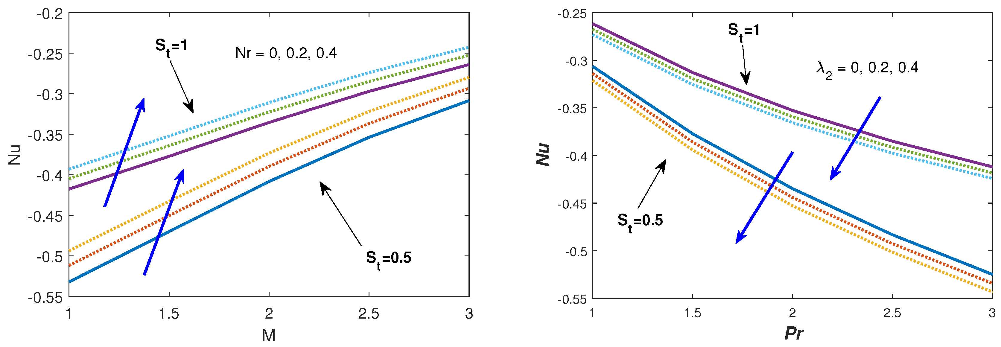
Effect of Lewis number () in nano-fluid slip condition on nano-fluid concentration profile is shown in Figure 13. Increase in Lewis number makes the boundary layer thinner. Lewis number is directly proportional to the Schmidt number and inversely proportional to the Brownian diffusion coefficient, which will cause the solute boundary layer to become‘thinner. Figure 14 exhibits the nature of the Skin friction coefficient with the magnetic, hydrodynamic slips and buoyancy parameters. We observed in Figure 14 that increase in the magnetic field strength M and strongly suppresses the Skin friction coefficient. Skin friction coefficient on the stretching surface is significantly enhanced with the increase in the values of the hydrodynamic slip parameters, thermal buoyancy and solutal buoyancy parameters. Effect of M, , , and thermal slip on Nusselt number are shown in Figure 15. We noticed in this figure that the effect of thermal slip () on Nusselt number increases with the increasing values of magnetic and thermal radiation parameters, while it decreases with increasing values of buoyancy parameter and Prandtl number. From the figures, above, we see that in the existence of the hydrodynamic, thermal, solute and nano-fluid slip the velocity, temperature, solute concentration and nano-fluid volume fraction boundary layers all increased.
5. Conclusions
The present study investigated the axisymmetric MHD buoyant nano-fluid incompressible viscous electrically conducting flow in the presence of multiple slips, chemical reaction and thermal radiation over a stretching sheet. The current study leads to the following conclusions:
- In the existence of the hydrodynamic, thermal, solute and nano-fluid slip the velocity, temperature, solute concentration and nano-fluid volume fraction boundary layers increases.
- The radial velocity profile decreases while temperature and solute concentration increases with the increase in magnetic field and slip conditions.
- The velocity profile increases with increasing buoyancy parameters ().
- After enhancement of magnetic and thermal radiation parameter the effect of thermal slip for temperature profile increased the boundary layer.
- Solute concentration decreases with an increase in the stretching parameter, solutal slip, Schmidt number and chemical reaction parameter.
- The nano-fluid volume fraction profile retards with large values of Brownian motion parameter and Lewis number.
- Nusselt number increases in the presence of thermal slip with the increasing values of magnetic and thermal radiation parameters. Whereas, the effect is reversed for enhancing the values of solutal buoyancy parameter and Prandtl number.
Author Contributions
All authors contributed equally.
Funding
This research was funded by National Natural Science Foundation of China No. [11971386].
Conflicts of Interest
The authors declare no conflict of interest.
Nomenclature
| u,w | velocity components |
| B | magnetic field strength |
| uniform magnetic field strength | |
| Brownian parameter | |
| Schmidt number | |
| thermophoresis parameter | |
| Lewis number | |
| heat flux | |
| Brownian diffusion | |
| thermophoretic diffusion | |
| solute parameter | |
| chemical reaction | |
| constant temperature | |
| nanoparticle volume fraction | |
| ambient temperature | |
| ambient nanoparticle volume fraction | |
| M | magnetic parameter |
| Prandtl number | |
| thermal radiation | |
| a constant | |
| n | power-law exponent |
| hydrodynamic slip | |
| thermal slip | |
| solute slip | |
| nano-fluid slip | |
| temperature slip factor | |
| solutal concentration slip factor | |
| nanoparticle concentration slip factor | |
| mean absorbtion coefficient |
Greek Symbol
| ratio of nanoparticle heat capacity | |
| kinetic viscosity | |
| electric conductivity | |
| Stefan-Boltzmann constant | |
| thermal diffusivity | |
| viscosity of the fluid | |
| solute concentration | |
| chemical reaction | |
| ambient solute concentration | |
| Buoyancy parameters |
References
- Choi, S.U.; Eastman, J.A. Enhancing Thermal Conductivity of Fluids with Nanoparticles; Technical Report; Argonne National Lab.: Springfield, IL, USA, 1995. [Google Scholar]
- Buongiorno, J. Convective transport in nanofluids. J. Heat Transf. 2006, 128, 240–250. [Google Scholar] [CrossRef]
- Turkyilmazoglu, M. Exact analytical solutions for heat and mass transfer of MHD slip flow in nanofluids. Chem. Eng. Sci. 2012, 84, 182–187. [Google Scholar] [CrossRef]
- Kandelousi, M.S. Nanofluid Heat and Mass Transfer in Engineering Problems; BoD-Books on Demand: Norderstedt, Germany, 2017. [Google Scholar]
- Sheikholeslami, M.; Shamlooei, M.; Moradi, R. Numerical simulation for heat transfer intensification of nanofluid in a porous curved enclosure considering shape effect of Fe3O4 nanoparticles. Chem. Eng. Process. Intensif. 2018, 124, 71–82. [Google Scholar] [CrossRef]
- Sheikholeslami, M.; Shehzad, S. Magnetohydrodynamic nanofluid convection in a porous enclosure considering heat flux boundary condition. Int. J. Heat Mass Transf. 2017, 106, 1261–1269. [Google Scholar] [CrossRef]
- Sheikholeslami, M.; Sadoughi, M. Simulation of CuO-water nanofluid heat transfer enhancement in presence of melting surface. Int. J. Heat Mass Transf. 2018, 116, 909–919. [Google Scholar] [CrossRef]
- Ali Lund, L.; Omar, Z.; Khan, I.; Raza, J.; Bakouri, M.; Tlili, I. Stability Analysis of Darcy-Forchheimer Flow of Casson Type Nanofluid Over an Exponential Sheet: Investigation of Critical Points. Symmetry 2019, 11, 412. [Google Scholar] [CrossRef]
- Kuznetsov, A.; Nield, D. The Cheng–Minkowycz problem for natural convective boundary layer flow in a porous medium saturated by a nanofluid: A revised model. Int. J. Heat Mass Transf. 2013, 65, 682–685. [Google Scholar] [CrossRef]
- Salleh, S.N.A.; Bachok, N.; Arifin, N.M.; Ali, F.M. Numerical Analysis of Boundary Layer Flow Adjacent to a Thin Needle in Nanofluid with the Presence of Heat Source and Chemical Reaction. Symmetry 2019, 11, 543. [Google Scholar] [CrossRef]
- Kuznetsov, A.; Nield, D. Natural convective boundary-layer flow of a nanofluid past a vertical plate. Int. J. Therm. Sci. 2010, 49, 243–247. [Google Scholar] [CrossRef]
- Nield, D.; Kuznetsov, A. The Cheng–Minkowycz problem for natural convective boundary-layer flow in a porous medium saturated by a nanofluid. Int. J. Heat Mass Transf. 2009, 52, 5792–5795. [Google Scholar] [CrossRef]
- Bachok, N.; Ishak, A.; Pop, I. Boundary-layer flow of nanofluids over a moving surface in a flowing fluid. Int. J. Therm. Sci. 2010, 49, 1663–1668. [Google Scholar] [CrossRef]
- Rashidi, M.M.; Nasiri, M.; Khezerloo, M.; Laraqi, N. Numerical investigation of magnetic field effect on mixed convection heat transfer of nanofluid in a channel with sinusoidal walls. J. Magn. Magn. Mater. 2016, 401, 159–168. [Google Scholar] [CrossRef]
- Sheikholeslami, M.; Ganji, D. Numerical investigation for two phase modeling of nanofluid in a rotating system with permeable sheet. J. Mol. Liq. 2014, 194, 13–19. [Google Scholar] [CrossRef]
- Hatami, M.; Sheikholeslami, M.; Ganji, D. Nanofluid flow and heat transfer in an asymmetric porous channel with expanding or contracting wall. J. Mol. Liq. 2014, 195, 230–239. [Google Scholar] [CrossRef]
- Soundalgekar, V.; Gupta, S.; Aranake, R. Free convection effects on MHD Stokes problem for a vertical plate. Nucl. Eng. Des. 1979, 51, 403–407. [Google Scholar] [CrossRef]
- Elbashbeshy, E. Heat and mass transfer along a vertical plate with variable surface tension and concentration in the presence of the magnetic field. Int. J. Eng. Sci. 1997, 35, 515–522. [Google Scholar] [CrossRef]
- Jena, S.; Mishra, S.; Dash, G. Chemical reaction effect on MHD Jeffery fluid flow over a stretching sheet through porous media with heat generation/absorption. Int. J. Appl. Comput. Math. 2017, 3, 1225–1238. [Google Scholar] [CrossRef]
- Ramzan, M.; Bilal, M.; Chung, J.D.; Mann, A. On MHD radiative Jeffery nanofluid flow with convective heat and mass boundary conditions. Neural Comput. Appl. 2018, 30, 2739–2748. [Google Scholar] [CrossRef]
- Alarifi, I.M.; Abokhalil, A.G.; Osman, M.; Lund, L.A.; Ayed, M.B.; Belmabrouk, H.; Tlili, I. MHD Flow and Heat Transfer over Vertical Stretching Sheet with Heat Sink or Source Effect. Symmetry 2019, 11, 297. [Google Scholar] [CrossRef]
- Najib, N.; Bachok, N.; Arifin, N.M.; Ishak, A. Stagnation point flow and mass transfer with chemical reaction past a stretching/shrinking cylinder. Sci. Rep. 2014, 4, 4178. [Google Scholar] [CrossRef]
- Mishra, S.; Dash, G.; Pattnaik, P. Flow of heat and mass transfer on MHD free convection in a micropolar fluid with heat source. Alex. Eng. J. 2015, 54, 681–689. [Google Scholar] [CrossRef]
- Zaimi, K.; Ishak, A.; Pop, I. Boundary layer flow and heat transfer over a nonlinearly permeable stretching/shrinking sheet in a nanofluid. Sci. Rep. 2014, 4, 4404. [Google Scholar] [CrossRef] [PubMed] [Green Version]
- Ahmed, J.; Mahmood, T.; Iqbal, Z.; Shahzad, A.; Ali, R. Axisymmetric flow and heat transfer over an unsteady stretching sheet in power law fluid. J. Mol. Liq. 2016, 221, 386–393. [Google Scholar] [CrossRef]
- Shahzad, A.; Ahmed, J.; Khan, M. On heat transfer analysis of axisymmetric flow of viscous fluid over a nonlinear radially stretching sheet. Alex. Eng. J. 2016, 55, 2423–2429. [Google Scholar] [CrossRef] [Green Version]
- Khan, I.; Alqahtani, A.M. MHD Nanofluids in a Permeable Channel with Porosity. Symmetry 2019, 11, 378. [Google Scholar] [CrossRef]
- Makinde, O.D.; Mabood, F.; Ibrahim, M.S. Chemically reacting on MHD boundary-layer flow of nanofluids over a non-linear stretching sheet with heat source/sink and thermal radiation. Therm. Sci. 2018, 22, 495–506. [Google Scholar] [CrossRef]
- Mabood, F.; Shateyi, S. Multiple Slip Effects on MHD Unsteady Flow Heat and Mass Transfer Impinging on Permeable Stretching Sheet with Radiation. Model. Simul. Eng. 2019, 2019, 3052790. [Google Scholar] [CrossRef]
- Nayak, B.; Mishra, S.; Krishna, G.G. Chemical reaction effect of an axisymmetric flow over radially stretched sheet. Propuls. Power Res. 2019, 8, 79–84. [Google Scholar] [CrossRef]
- Crane, L.J. Flow past a stretching plate. Z. FÜR Angew. Math. Und Phys. Zamp 1970, 21, 645–647. [Google Scholar] [CrossRef]
- Gireesha, B.; Ramesh, G.; Bagewadi, C. Heat transfer in MHD flow of a dusty fluid over a stretching sheet with viscous dissipation. J. Appl. Sci. Res. 2012, 3, 2392–2401. [Google Scholar]
- Jalil, M.; Asghar, S.; Yasmeen, S. An exact solution of MHD boundary layer flow of dusty fluid over a stretching surface. Math. Probl. Eng. 2017, 2017, 2307469. [Google Scholar] [CrossRef]
- Nawaz, M.; Hayat, T. Axisymmetric stagnation-point flow of nanofluid over a stretching surface. Adv. Appl. Math. Mech. 2014, 6, 220–232. [Google Scholar] [CrossRef]
- Mustafa, M.; Khan, J.A.; Hayat, T.; Alsaedi, A. Analytical and numerical solutions for axisymmetric flow of nanofluid due to non-linearly stretching sheet. Int. J. Non-Linear Mech. 2015, 71, 22–29. [Google Scholar] [CrossRef]
- Mustafa, M.; Hayat, T.; Alsaedi, A. Axisymmetric flow of a nanofluid over a radially stretching sheet with convective boundary conditions. Curr. Nanosci. 2012, 8, 328–334. [Google Scholar] [CrossRef]
- Pal, D. Heat and mass transfer in stagnation-point flow towards a stretching surface in the presence of buoyancy force and thermal radiation. Meccanica 2009, 44, 145–158. [Google Scholar] [CrossRef]
- Almakki, M.; Dey, S.; Mondal, S.; Sibanda, P. On Unsteady Three-Dimensional Axisymmetric MHD Nanofluid Flow with Entropy Generation and Thermo-Diffusion Effects. Entropy 2017, 19, 168. [Google Scholar] [CrossRef]
- Mabood, F.; Khan, W.; Ismail, A.M. Multiple slips effects on MHD Casson fluid flow in porous media with radiation and chemical reaction. Can. J. Phys. 2015, 94, 26–34. [Google Scholar] [CrossRef]
- Gupta, D.; Kumar, L.; Bég, O.A.; Singh, B. Finite-element simulation of mixed convection flow of micropolar fluid over a shrinking sheet with thermal radiation. Proc. Inst. Mech. Eng. Part J. Process. Mech. Eng. 2014, 228, 61–72. [Google Scholar] [CrossRef]
- Gupta, D.; Kumar, L.; Bég, O.A.; Singh, B. Finite element analysis of MHD flow of micropolar fluid over a shrinking sheet with a convective surface boundary condition. J. Eng. Thermophys. 2018, 27, 202–220. [Google Scholar] [CrossRef]
- Madhu, M.; Kishan, N. Finite Element Analysis of MHD viscoelastic nanofluid flow over a stretching sheet with radiation. Procedia Eng. 2015, 127, 432–439. [Google Scholar] [CrossRef]
- Mabood, F.; Das, K. Melting heat transfer on hydromagnetic flow of a nanofluid over a stretching sheet with radiation and second-order slip. Eur. Phys. J. Plus 2016, 131, 3. [Google Scholar] [CrossRef]
- Ali, M.E. Heat transfer characteristics of a continuous stretching surface. Wärme-und Stoffübertragung 1994, 29, 227–234. [Google Scholar] [CrossRef]
Figure 1.
Physical configuration and coordinate system.

Figure 2.
Effect of M on velocity distribution in the presence and absence of hydrodynamic slip condition .
Figure 2.
Effect of M on velocity distribution in the presence and absence of hydrodynamic slip condition .
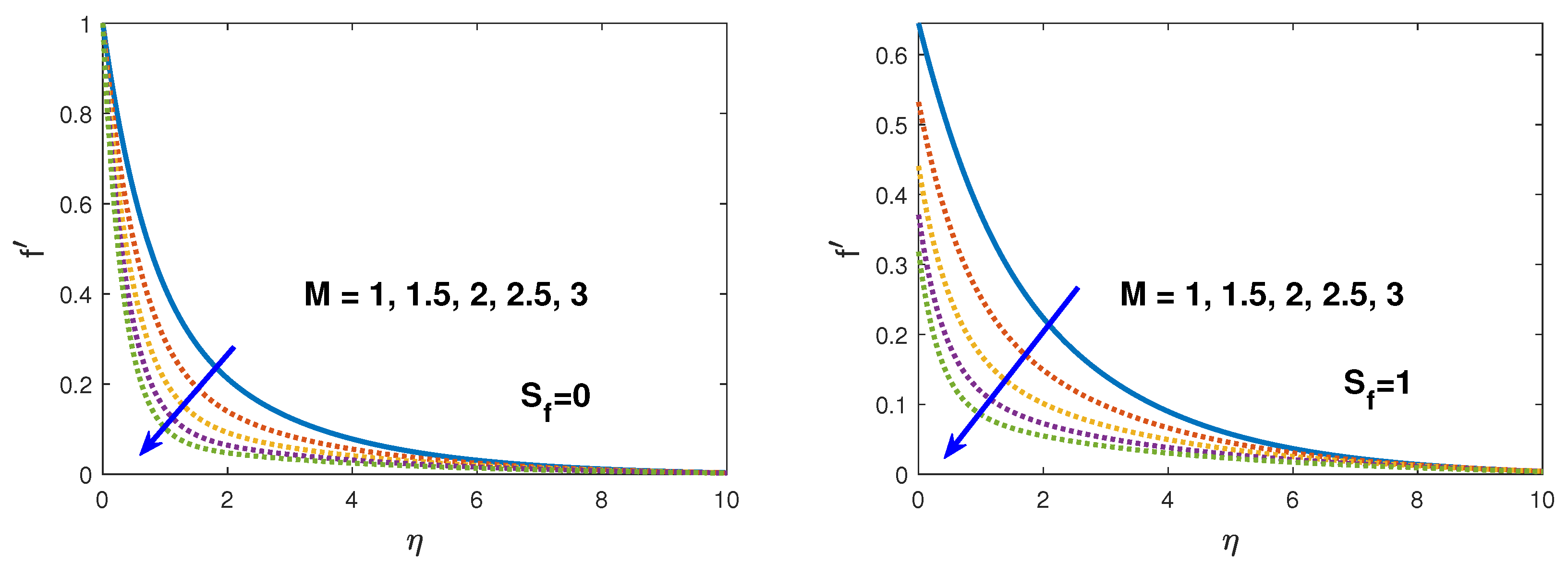
Figure 3.
Effect of M on temperature distribution in the presence and absence of thermal slip condition .
Figure 3.
Effect of M on temperature distribution in the presence and absence of thermal slip condition .
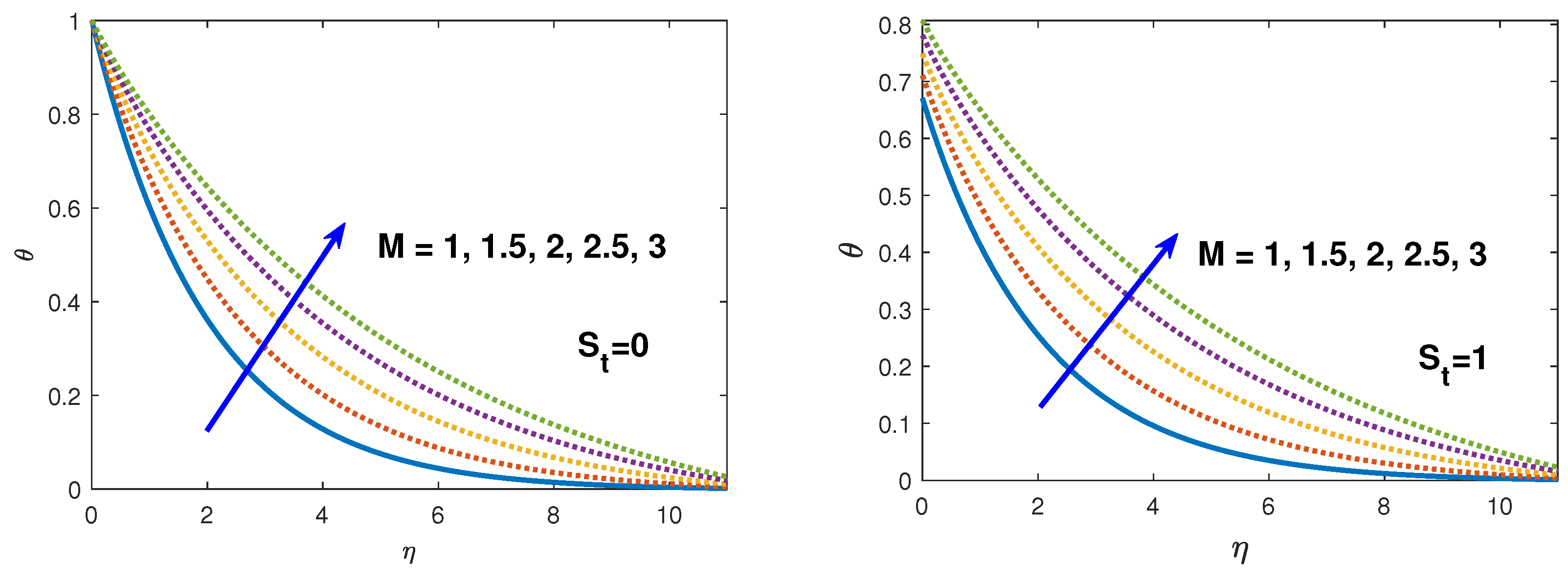
Figure 4.
Effect of M on solute concentration in the presence and absence of solute slip condition .
Figure 4.
Effect of M on solute concentration in the presence and absence of solute slip condition .

Figure 5.
Effect of on velocity distribution in the presence and absence of solute slip condition .
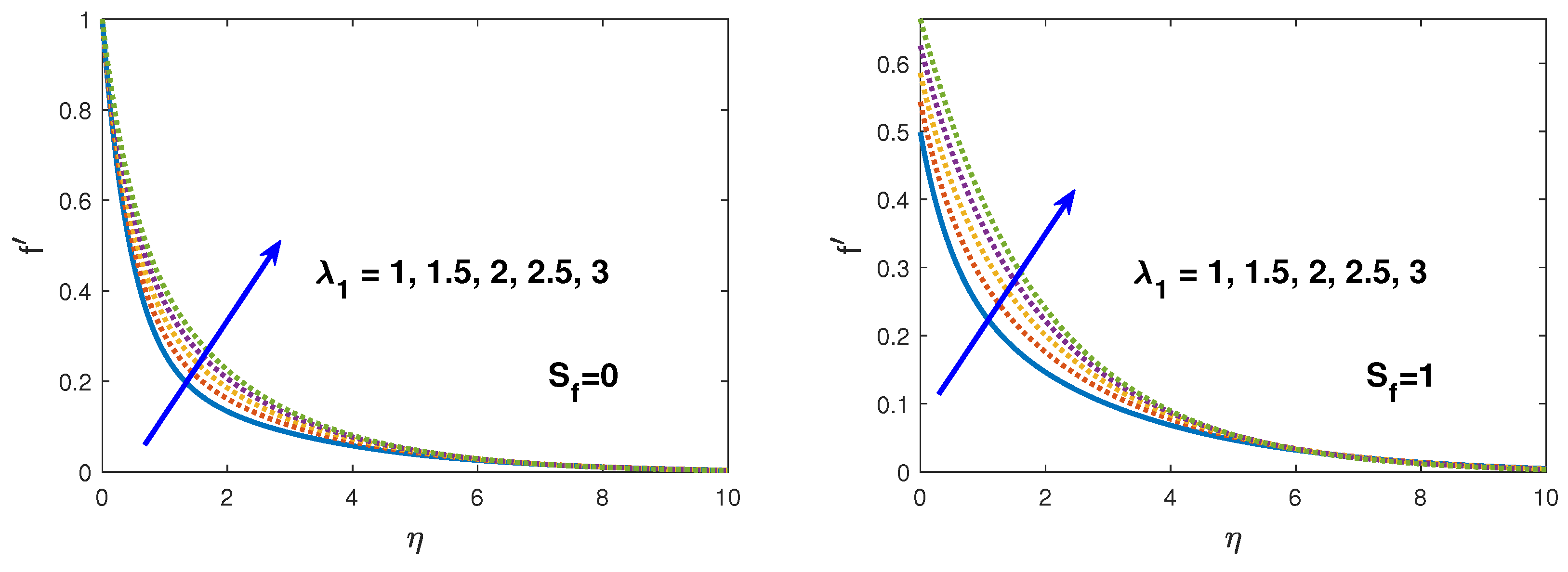
Figure 6.
Effect of on velocity distribution in the presence and absence of solute slip condition .
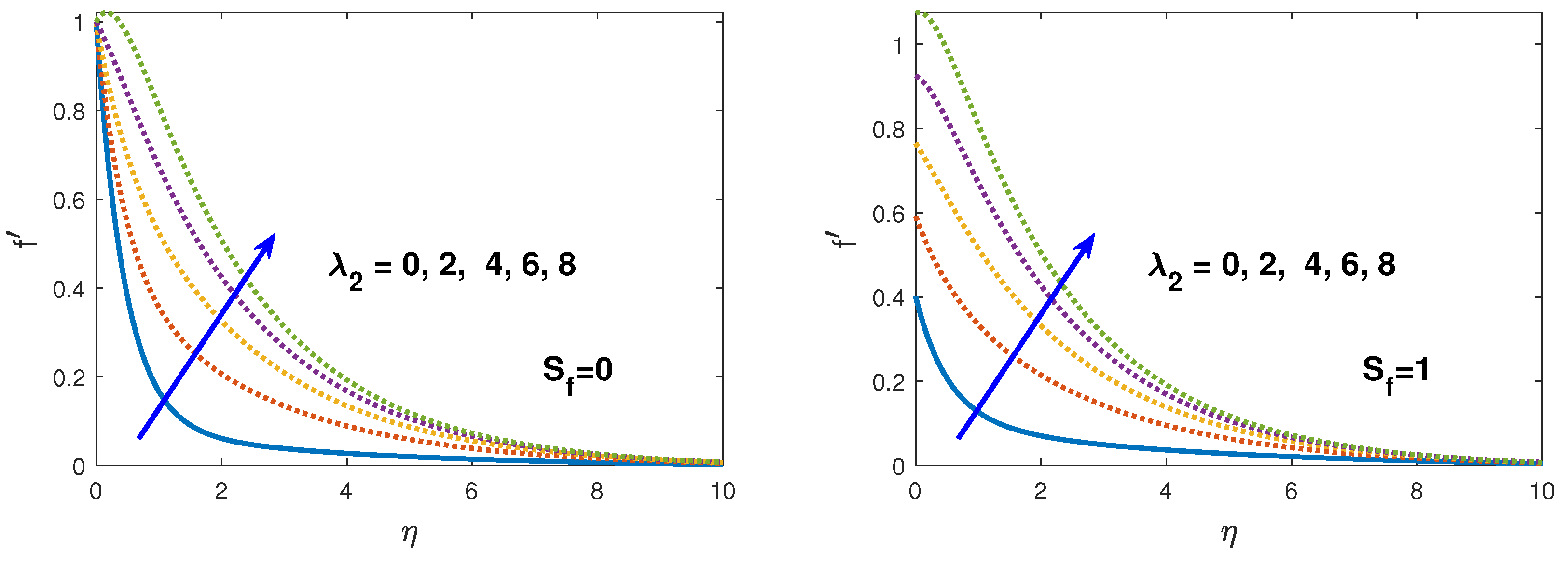
Figure 7.
Effect of on velocity distribution in the presence and absence of solute slip condition .
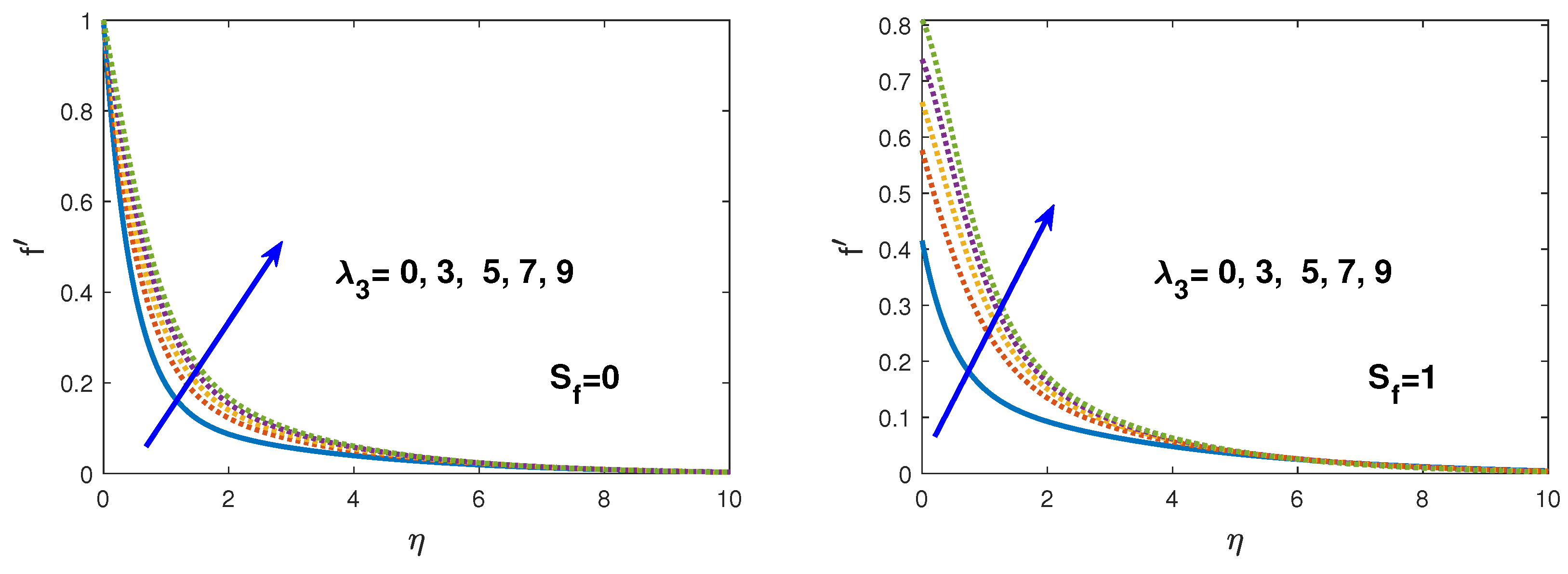
Figure 8.
Effect of on temperature distribution in the presence and absence of thermal slip condition .
Figure 8.
Effect of on temperature distribution in the presence and absence of thermal slip condition .
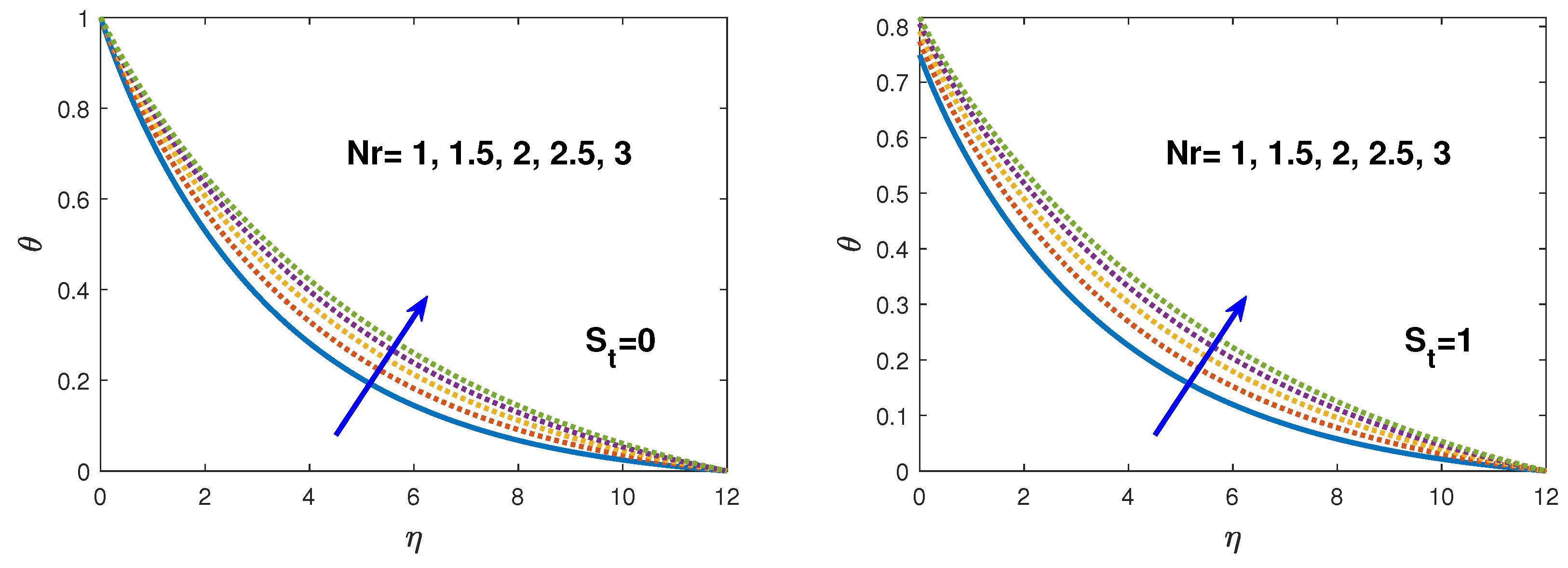
Figure 9.
Effect of on nano-fluid volume fraction profile in the presence and absence of nano-fluid slip condition .
Figure 9.
Effect of on nano-fluid volume fraction profile in the presence and absence of nano-fluid slip condition .
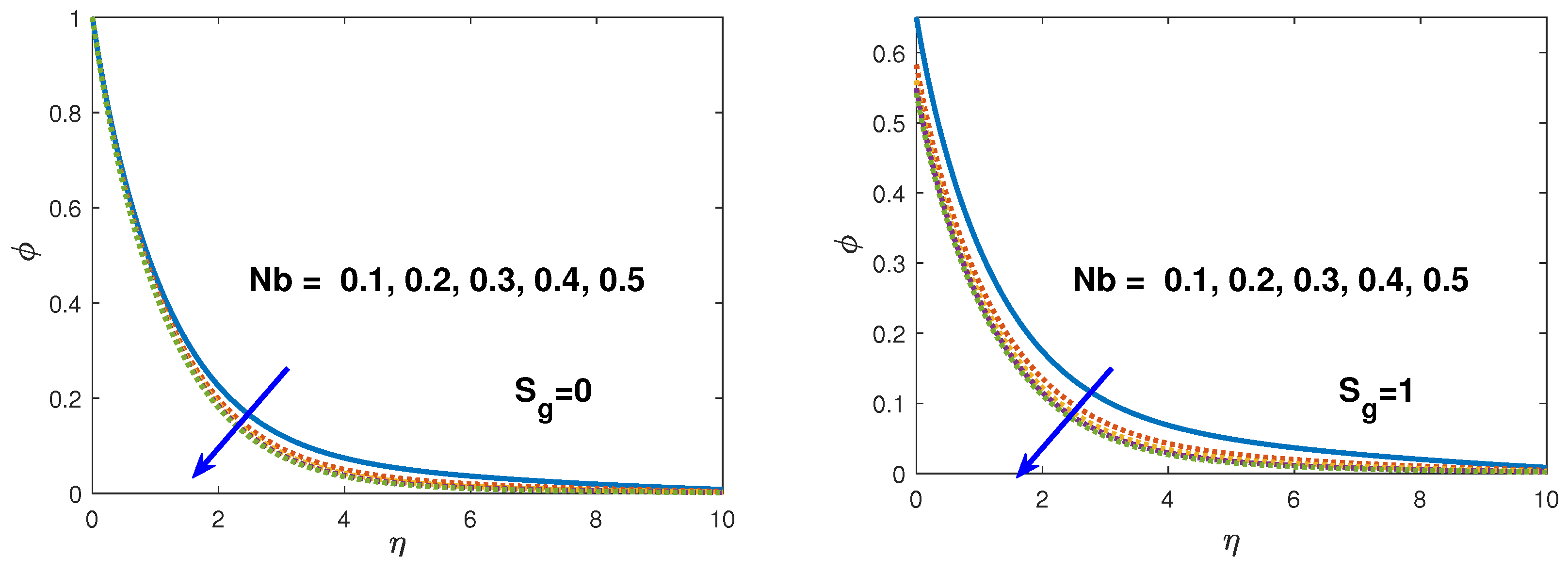
Figure 10.
Effect of n on solute concentration in the presence and absence of solutal slip condition .
Figure 10.
Effect of n on solute concentration in the presence and absence of solutal slip condition .
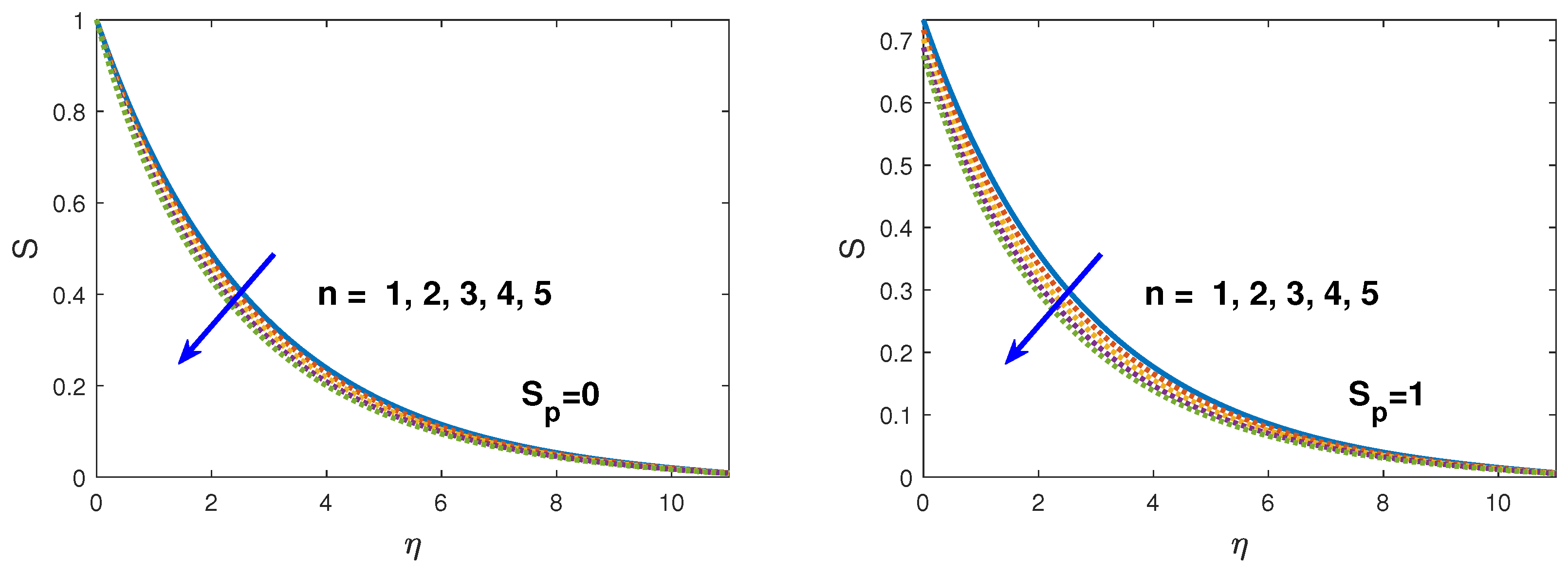
Figure 11.
Effect of on solute concentration in the presence and absence of solute slip condition .
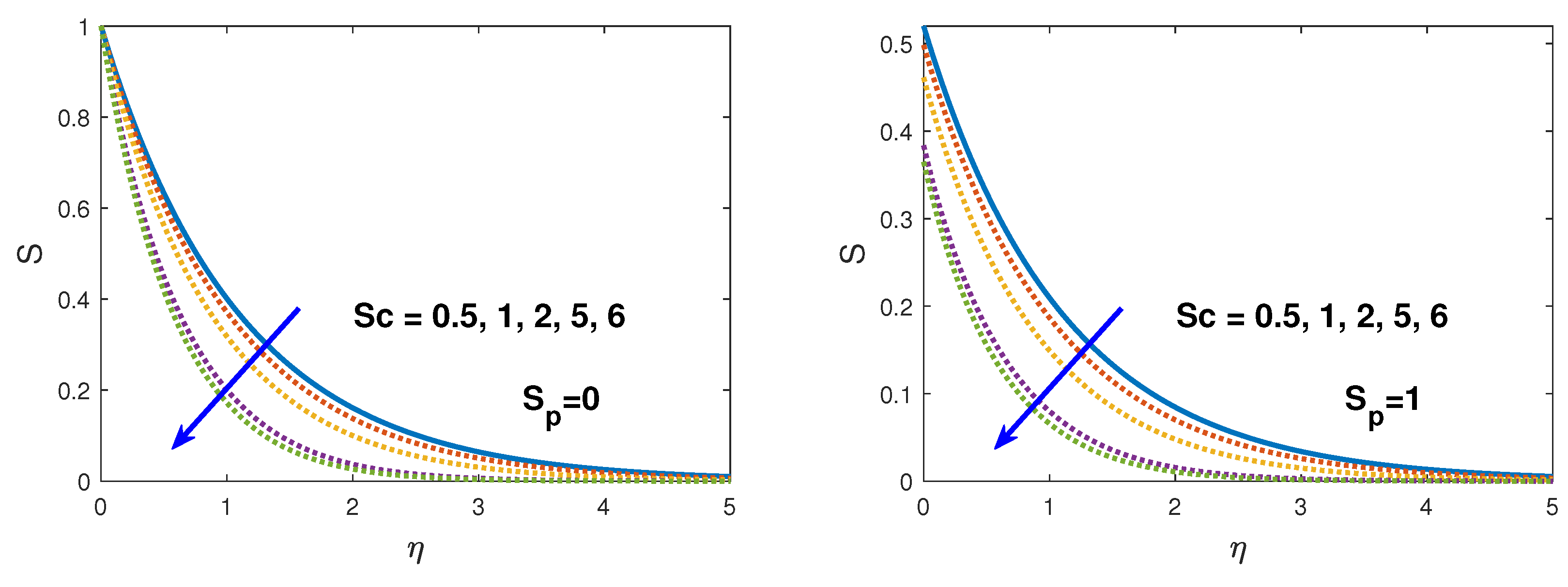
Figure 12.
Effect of on solute concentration in the presence and absence of solute slip condition .

Figure 13.
Effect of on nano-fluid volume fraction profile in the presence and absence of nano-fluid slip condition .
Figure 13.
Effect of on nano-fluid volume fraction profile in the presence and absence of nano-fluid slip condition .
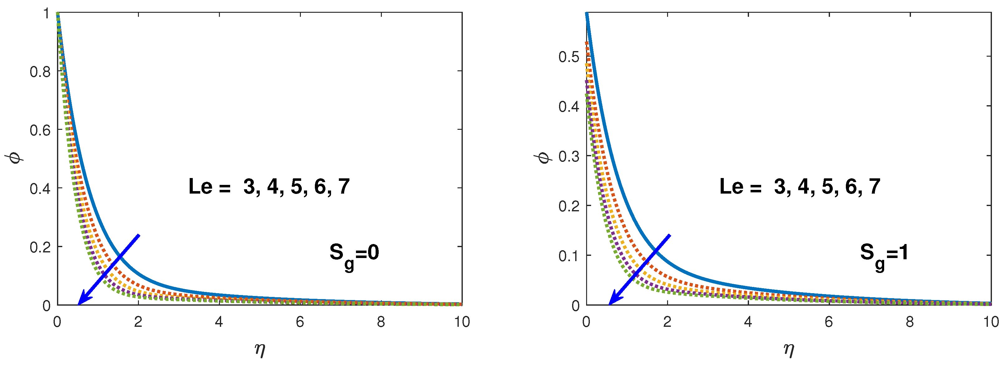
Figure 14.
Effect of M, and in hydrodynamic slip condition on Skin friction coefficient.

Figure 15.
Effect of M, , and in thermal slip condition on Nusselt number.

Table 1.
Convergence results of FEM with the variation of number of elements (, , , , , , , , , , , ).
Table 1.
Convergence results of FEM with the variation of number of elements (, , , , , , , , , , , ).
| Number of Elements | |||||
|---|---|---|---|---|---|
| 40 | 0.5275 | 0.0670 | 0.3416 | 0.2898 | 0.0546 |
| 80 | 0.5305 | 0.0670 | 0.3409 | 0.2898 | 0.0546 |
| 120 | 0.5310 | 0.0670 | 0.3408 | 0.2898 | 0.0547 |
| 160 | 0.5312 | 0.0670 | 0.3407 | 0.2898 | 0.0547 |
| 200 | 0.5313 | 0.0670 | 0.3407 | 0.2898 | 0.0547 |
| 240 | 0.5313 | 0.0670 | 0.3407 | 0.2898 | 0.0547 |
| 280 | 0.5314 | 0.0670 | 0.3407 | 0.2898 | 0.0547 |
| 320 | 0.5314 | 0.0670 | 0.3407 | 0.2898 | 0.0547 |
Table 2.
Comparison of the FEM solution with the exact solution of Crane [31].
Table 2.
Comparison of the FEM solution with the exact solution of Crane [31].
| Crane [31] | FEM | Crane [31] | FEM | ||
|---|---|---|---|---|---|
| 0 | 1 | 1 | 7 | 0.0009 | 0.0009 |
| 1 | 0.3679 | 0.3679 | 8 | 0.0003 | 0.0003 |
| 2 | 0.1353 | 0.1353 | 9 | 0.0001 | 0.0001 |
| 3 | 0.0498 | 0.0498 | 10 | 0.0000 | 0.0000 |
| 4 | 0.0183 | 0.0183 | 11 | 0.0000 | 0.0000 |
| 5 | 0.0067 | 0.0067 | 12 | 0.0000 | 0.0000 |
| 6 | 0.0025 | 0.0025 | 13,14,15 | 0.0000 | 0.0000 |
Table 3.
Comparison of skin friction coefficient for different values of M.
| M | Gireesha et al. [32] | Mudassar et al. [33] Exact Solution (a) | FEM (Our Results) (b) | Error in % |
|---|---|---|---|---|
| 0.0 | 1.000 | 1.000000 | 1.0000080 | 0.00080 |
| 0.2 | 1.095 | 1.095445 | 1.0954458 | 0.00007 |
| 0.5 | 1.224 | 1.224745 | 1.2247446 | 0.00003 |
| 1.0 | 1.414 | 1.414214 | 1.4142132 | 0.00006 |
| 1.2 | 1.483 | 1.483240 | 1.4832393 | 0.00005 |
| 1.5 | 1.581 | 1.581139 | 1.5811384 | 0.00004 |
| 2.0 | 1.732 | 1.732051 | 1.7320504 | 0.00003 |
Table 4.
Comparison of for various values of M when and when .
| M | Mabood and Das [43] | Fazle [29] | FEM (Present) | Ali [44] | Fazle [29] | FEM (Present) | |
|---|---|---|---|---|---|---|---|
| 0 | −1.000008 | −1.0000084 | −1.0000082 | - | - | - | - |
| 1 | 1.4142135 | 1.41421356 | 1.41421353 | - | - | - | - |
| 5 | 2.4494897 | 2.44948974 | 2.44948963 | 0.72 | 0.8058 | 0.8088 | 0.8088 |
| 10 | 3.3166247 | 3.31662479 | 3.31662463 | 1 | 0.9691 | 1.0000 | 1.0000 |
| 50 | 7.1414284 | 7.14142843 | 7.14142839 | 3 | 1.9144 | 1.9237 | 1.9237 |
| 100 | 10.049875 | 10.0498756 | 10.0498751 | 10 | 3.7006 | 3.7207 | 3.7207 |
| 500 | 22.383029 | 22.3830293 | 22.3830283 | - | - | - | - |
| 1000 | 31.638584 | 31.6385840 | 31.6385833 | - | - | - | - |
Table 5.
Computed values of skin fraction coefficient, heat transfer coefficient and mass transfer coefficient for , , , , , , , , , ).
Table 5.
Computed values of skin fraction coefficient, heat transfer coefficient and mass transfer coefficient for , , , , , , , , , ).
| M | |||||||||
|---|---|---|---|---|---|---|---|---|---|
| 1 | −0.51871906 | −0.39914438 | −0.33469636 | ||||||
| 1.5 | 0.1 | 0.773 | 1 | 0.4 | 0.4 | 0.4 | −0.70007439 | −0.34330234 | −0.32039573 |
| 2 | −0.86037797 | −0.29152259 | −0.30916534 | ||||||
| 0.1 | −0.86037797 | −0.29152259 | −0.30916534 | ||||||
| 2 | 0.5 | 0.773 | 1 | 0.4 | 0.4 | 0.4 | −0.87456687 | −0.27774645 | −0.53903314 |
| 1 | −0.88233600 | −0.27260197 | −0.67751871 | ||||||
| 2 | −0.86809394 | −0.46620439 | −0.30740431 | ||||||
| 2 | 0.1 | 3 | 1 | 0.4 | 0.4 | 0.4 | −0.87169999 | −0.55675321 | −0.30668459 |
| 4 | −0.87422111 | −0.62457605 | −0.30622757 | ||||||
| 2 | −0.85775278 | −0.23671739 | −0.30981895 | ||||||
| 2 | 0.1 | 0.773 | 3 | 0.4 | 0.4 | 0.4 | −0.85618413 | −0.20495708 | −0.31022032 |
| 4 | −0.85513340 | −0.18408657 | −0.31049339 | ||||||
| 0.5 | −0.84545297 | −0.29890014 | −0.31058477 | ||||||
| 1 | −0.77396002 | −0.32928379 | −0.31696545 | ||||||
| 1.5 | −0.70660726 | −0.35282310 | −0.32248200 | ||||||
| 0.5 | −0.84570667 | −0.29845530 | −0.31051308 | ||||||
| 0.7 | −0.81650214 | −0.31161198 | −0.31317081 | ||||||
| 0.9 | −0.78749387 | −0.32389598 | −0.31577681 | ||||||
| 0.4 | −0.86037797 | −0.29152259 | −0.30916534 | ||||||
| 0.8 | −0.82636008 | −0.30157756 | −0.31127720 | ||||||
| 1.2 | −0.79384196 | −0.31065228 | −0.31323236 |
© 2019 by the authors. Licensee MDPI, Basel, Switzerland. This article is an open access article distributed under the terms and conditions of the Creative Commons Attribution (CC BY) license (http://creativecommons.org/licenses/by/4.0/).
Share and Cite
MDPI and ACS Style
Khan, S.A.; Nie, Y.; Ali, B. Multiple Slip Effects on Magnetohydrodynamic Axisymmetric Buoyant Nanofluid Flow above a Stretching Sheet with Radiation and Chemical Reaction. Symmetry 2019, 11, 1171. https://doi.org/10.3390/sym11091171
AMA Style
Khan SA, Nie Y, Ali B. Multiple Slip Effects on Magnetohydrodynamic Axisymmetric Buoyant Nanofluid Flow above a Stretching Sheet with Radiation and Chemical Reaction. Symmetry. 2019; 11(9):1171. https://doi.org/10.3390/sym11091171
Chicago/Turabian StyleKhan, Shahid Ali, Yufeng Nie, and Bagh Ali. 2019. "Multiple Slip Effects on Magnetohydrodynamic Axisymmetric Buoyant Nanofluid Flow above a Stretching Sheet with Radiation and Chemical Reaction" Symmetry 11, no. 9: 1171. https://doi.org/10.3390/sym11091171
Note that from the first issue of 2016, this journal uses article numbers instead of page numbers. See further details here.