Article

Critically-Finite Dynamics on the Icosahedron

Department of Mathematics and Statistics, California State University, Long Beach, CA 90840, USA
Symmetry 2020, 12(1), 177; https://doi.org/10.3390/sym12010177
Submission received: 11 December 2019 / Revised: 10 January 2020 / Accepted: 16 January 2020 / Published: 19 January 2020
(This article belongs to the Special Issue Symmetry and Dynamical Systems)

Abstract

:
A recent effort used two rational maps on the Riemann sphere to produce polyhedral structures with properties exemplified by a soccer ball. A key feature of these maps is their respect for the rotational symmetries of the icosahedron. The present article shows how to build such “dynamical polyhedra” for other icosahedral maps. First, algebra associated with the icosahedron determines a special family of maps with 60 periodic critical points. The topological behavior of each map is then worked out and results in a geometric algorithm out of which emerges a system of edges—the dynamical polyhedron—in natural correspondence to a map’s topology. It does so in a procedure that is more robust than the earlier implementation. The descriptions of the maps’ geometric behavior fall into combinatorial classes the presentation of which concludes the paper.

Graphical Abstract

1. Overview

A polynomial map on the projective space CP 1 —the Riemann sphere—is given by an ordered pair of polynomials
f ( x , y ) = ( P ( x , y ) , Q ( x , y ) ) .
Being well-defined on the complex projective line requires the coordinates ( x , y ) to be homogeneous, meaning that each term in P and Q has the same total degree—the sum of the exponents. This total degree is the degree of f. By introducing an inhomogeneous coordinate z = x y , we can express f as a rational map in one variable on the space C = { ( x , y )   |   y 0 } :
f ( z ) = P ( z , 1 ) Q ( z , 1 ) .
At the core of the quintic-solving algorithm devised by Doyle and McMullen is the dynamics of a special rational map with the symmetries of the icosahedron [1]. Their degree-11 map on the Riemann sphere has a critical set that coincides with the 20 vertices of the regular dodecahedron—a special icosahedral orbit. There is also a map of degree 19 under which the 12 icosahedral vertices are critical.
A key property of these maps is a strong form of critical-finiteness: the critical points are periodic. The critical set of a map f = ( u , v ) consists of the points ( a , b ) where no neighborhood exists on which the map is invertible, a condition equivalent to
u x ( a , b ) = v x ( a , b ) = 0 .
The behavior of a map’s critical orbit—where the critical points go when the map is applied iteratively—bears strongly on the map’s global dynamics (See [2], Chapter 9). In the particular case of periodic critical points, their basins of attraction have full measure on the sphere. An attracting cycle’s basin of attraction contains all points whose dynamical orbits asymptotically approach the cycle. Moreover, each map gives rise to a forward invariant polyhedral structure of edges relative to which the map has an elegant geometric description. Due to the critical sets’ achiral arrangements, the edges lie along great circles of reflective icosahedral symmetry. Indeed, the maps are also symmetric under reflection along the edges. Associated with the “11-map” is a dodecahedron and with the 19-map an icosahedron.
A recent unexpected discovery revealed the existence of two icosahedrally-symmetric maps with periodic critical sets of generic size, that is, each critical set is a 60-point orbit under the icosahedral group [3]. The configurations of critical points take the form, in one case, of a soccer ball’s vertices and, in the other, of the vertices on a type of dual soccer ball. For a 60-point critical set, the core question of the current investigation is whether there are dynamically natural edges between the vertices. A combinatorial structure of this kind has two important properties: (1) invariance as a collection of points when the respective map is applied and (2) the wherewithal for describing in geometric terms the respective map’s behavior. The previous effort showed a way of constructing such a “dynamical polyhedron” for the soccer-ball map.
In the present undertaking, we will determine all icosahedral maps with internally periodic critical sets of size 60; ‘internal’ means that the map permutes the critical points. We then study two special cases in some detail, describing the dynamical behavior in geometric terms. Subsequent discussion turns to the heart of the problem: edge-constructions for dynamical polyhedra. The critical sets, hence the systems of edges, for most of the maps form chiral configurations.
On terminology and graphics: “Facts” and graphical output are computational results generated by Mathematica. Notebooks that implement the construction are available at [4].

2. Preliminaries: Icosahedral Geometry, Invariants, and Equivariants

Detailed descriptions of the geometric and algebraic structures associated with the icosahedron appear elsewhere [1,5]. For a brief summary of the relevant background, see [3]. The features essential to the topic at hand will now be discussed.
First, choose coordinates in CP 1 so that a pair of antipodal icosahedral vertices are at [ 0 , 1 ] and [ 1 , 0 ] where square brackets indicate projective coordinates; that is, the point
[ x , y ] = { ( α   x , α   y )   |   α C ( 0 , 0 ) }
in CP 1 is an equivalence class in C 2 . Using an inhomogeneous coordinate z on the complex line { y   |   y 0 } such that
[ z , 1 ] = x y , 1 = [ x , y ] ,
the respective locations of these two vertices are 0 and . Rendered on the sphere, the two points can be taken to be the south and north poles. Placing a third vertex on the real axis at 1 + 5 2 determines the locations of the remaining vertices:
V = { 0 , 1 2 ( 1 5 ) , 1 2 ( 1 + 5 ) , 5 + 5 i 10 ( 5 + 5 ) 2 ( 5 5 ) , 5 + 5 i 10 ( 5 + 5 ) 2 ( 5 + 5 ) , 10 + 2 5 + 5 i 2 ( 5 + 5 ) i 10 ( 5 + 5 ) 20 + 4 5 , 2 ( 5 + 5 ) + 5 i 2 ( 5 + 5 ) i 10 ( 5 + 5 ) 4 ( 5 5 ) , 5 + 5 + i 10 ( 5 + 5 ) 2 ( 5 5 ) , 5 + 5 + i 10 ( 5 + 5 ) 2 ( 5 + 5 ) , 10 + 2 5 5 i 2 ( 5 + 5 ) + i 10 ( 5 + 5 ) 20 + 4 5 , 2 ( 5 + 5 ) 5 i 2 ( 5 + 5 ) + i 10 ( 5 + 5 ) 4 ( 5 5 ) } .
By taking triples of vertices that belong to a face of the icosahedron, we obtain 20 face-centers. Similarly, from pairs of vertices that are endpoints of icosahedral edges that bound a face, we compute 30 edge-midpoints.
Taking the set V to be the regular icosahedron, its orientation-preserving symmetries form a group consisting of 60 rotations that act on the Riemann sphere CP 1 . The icosahedral group I is isomorphic to the alternating group A 5 . Furthermore, I can be extended by a reflection through a great circle to a group I ˜ of 120 transformations half of which are orientation-reversing—that is, anti-holomorphic.
The I -invariant polynomials form an algebraic object known as a ring. Three forms F, H, and T generate this ring. Each generator vanishes on a special icosahedral orbit, that is, F = 0 at the vertices, H = 0 at the face-centers, and T = 0 at the edge-midpoints. Accordingly, the generating invariants have respective degrees 12, 20, and 30. Since I permutes the vertices, the polynomial F ( x , y ) that takes the value zero exactly at each vertex is I -invariant. That is,
F ( A ( x , y ) ) = F ( x , y ) for   all   A I .
In homogeneous coordinates,
F ( x , y ) = x y ( x 10 11 x 5 y 5 y 10 ) .
Applying the same reasoning to the face-centers and edge-midpoints yields I -invariants of degrees 20 and 30:
H ( x , y ) = x 20 + 228 x 15 y 5 + 494 x 10 y 10 228 x 5 y 15 + y 20 , T ( x , y ) = x 30 522 x 25 y 5 10 , 005 x 20 y 10 10 , 005 x 10 y 20 + 522 x 5 y 25 + y 30 .
An important fact in other contexts is that the generating invariants satisfy an algebraic relation in degree 60:
T 2 = H 3 1728   F 5 .
Associated with an I -invariant G is an I -equivariant rational map— I -map for short—whose degree is one less than that of G. An equivariant is a map f that commutes with a group action A and thereby respects group orbits. In symbolic terms,
f B = B f for   all   B A
and the group orbit A ( x , y ) = { B ( x , y )   |   B A } maps to
f ( A ( x , y ) ) = A ( f ( x , y ) ) ,
also a group orbit. Accordingly, an I -map can be pushed down to a map on the quotient space CP 1 / I consisting of equivalence classes of group orbits. We will put this property to computational use below.
In the icosahedral case, maps of degrees 11 and 19 generate the module of I -maps over the ring of I -invariants. This module contains I -maps of the form
R · ϕ + S · η ,
where R and S are I -invariants such that the degrees of each product are the same. Generators for I -maps result from applying a differential operator to the I -invariants F and H:
ϕ ( x , y ) =   F y , F x = ( x 11 + 66 x 6 y 5 + 11 x y 10 , 11 x 10 y 66 x 5 y 6 y 11 ) , η ( x , y ) =   H y , H x = ( 20 ( 57 x 15 y 4 + 247 x 10 y 9 171 x 5 y 14 + y 19 ) , 20 ( x 19 + 171 x 14 y 5 + 247 x 9 y 10 57 x 4 y 15 ) ) .
Due to the relation (1), we need not include a map derived from the invariant T.

3. Rational Maps on CP1 as Branched Self-Covers

A map f : CP 1 CP 1 with a forward invariant critical set C f is a branched self-cover of CP 1 , meaning that, since C f f 1 ( C f ) ,
f : ( CP 1 f 1 ( C f ) ) ( CP 1 C f )
is a covering map. A basic problem set by William Thurston is to determine a condition on a branched self-cover f of CP 1 that reveals whether or not f is topologically conjugate to a rational map. Thurston formulated a negative result: a branched self-cover is not conjugate to a rational map when and only when a certain combinatorial obstruction exists [6].
In recent work, Dylan Thurston discovered a positive characterization for rationality ([7,8]). Central to the theory is an elastic graph spine G f in CP 1 C f the existence of which is necessary and sufficient for the self-cover to be conjugate to a rational map. (The full result applies to a class of maps that is larger than those with periodic critical points, but such maps are the focus here.) Put briefly, a “Thurston spine” is a graph (1) to which CP 1 C f can be continuously deformed and (2) with a length function—giving rise to an elastic energy—defined on its edges such that when f 1 is applied to the graph, the edges loosen in the sense of a decrease in elastic energy.
The cases of the 11-map, 19-map, and degree-31 soccer ball maps realize dynamical polyhedra with complementary antipodal behavior. That is, the sphere is carved into a cell-division with antipodal structure whose bounding edges form a graph G. Define a self-cover of CP 1 by stretching a cell onto the complement of its antipodal cell. Up to homotopy, the resulting map h is rational provided that it admits a Thurston spine. In private correspondence, Peter Doyle observes that the dual graph G ^ of G—essentially the dual polyhedron—gives such a spine. Backward iteration of h relaxes the edges of G ^ .
Taking inspiration from these examples, we’ll construct, for each map f with 60 internally periodic critical points, an approximation to a graph in CP 1 with dynamical integrity. Such a graph gives an f-invariant system of edges E f that encloses faces with 2, 3, and 5-fold symmetry and whose vertices are the critical points. Since the maps are rational, they admit a Thurston spine. However, we can turn the discussion around and conjecture that, for each dynamical polyhedron of a 31-map with its topological description as a self-cover of the sphere, there is a natural Thurston spine. Note that, in the description of the self-covering behavior, a face F maps to the complement of a cluster of faces that contains either F or its antipodal face. Perhaps such a spine can be built by taking an I -invariant graph that is dual to the polyhedral graph E f and thereby encloses the critical points.
In addition, self-coverings like the type discussed here might have a role to play in the problem of synchronization in a network. The difficulty there is to determine stochastic conditions acting on a population of agents that are favorable for the formation of consensus—a state which other states approach asymptotically through a dynamical process [9].

4. Icosahedral Maps with Periodic Critical Orbits

Our first task is to uncover each I -map f whose internally-periodic critical set C f consists of a single I -orbit of size 60. For such a critically-finite map, C f is a superattracting set; that is, the iterate f n that fixes each periodic critical point is topologically equivalent to a power map
( x , y ) α   ( x k , y k ) , k 2
on a neighborhood of ( 0 , 0 ) . Furthermore, the collective basins of attraction for the points in C f fill the sphere in the sense of measure.
As described in [3], maps with 60-point critical sets occur in degree 31 and the family of “31-maps” is given by
f ( a , b ) = a   H   ϕ + b   F   η .
To determine members of this family with periodic critical points, we follow a suggestion made by Peter Doyle and consider the maps induced on the quotient space Q = CP 1 / I . First, note that the quotient map
q : CP 1 Q
is realized, using homogeneous coordinates, by
( X , Y ) = q ( x , y ) = ( F ( x , y ) 5 , H ( x , y ) 3 ) .
Using an inhomogeneous parameter Z = X Y , an I -orbit is the collection of solutions z to
Z = F ( z ) 5 H ( z ) 3 .
Expressed diagrammatically (with the parameters suppressed), f is the lift of a map f ^ on Q :
CP 1 f CP 1 q q q q Q f ^ Q .
Letting
J f = u x u y v x v y
be the Jacobian matrix of f = ( u , v ) , the critical polynomial is C f = det J f and
C f = { C f = 0 }
is the critical set.
Invariant theory tells us that C f is I -invariant and thus expressible as a polynomial in F and H. Note that we can dispense with the invariant T in light of the degree-60 relation (1). Since C f has degree 60, it can be expressed in terms of the quotient coordinates X = F 5 and Y = H 3 .
Fact 1.
The critical polynomial of f descends to Q as
C f ^ = 4800   b   ( 12   a + 19   b ) X a   ( 11   a + 20   b ) Y .
Accordingly, C f ^ = { C f ^ = 0 } Q has the parametrization
Γ = ( a   ( 11   a + 20   b ) , 4800   b   ( 12   a + 19   b ) ) .
Note that, for each ( a , b ) , C f is a single I -orbit. Hence, C f ^ is a point in Q .
Now, we need to express the 31-maps f ^ on the quotient. First, note that composing an I -invariant with an I -map results in an I -invariant. In the present context, we obtain
f ^ ( X , Y ) = f ^ ( q ( x , y ) ) = q ( f ( x , y ) ) = ( F ( f ( x , y ) ) 5 , H ( f ( x , y ) ) 3 ) | ( F 5 , H 3 ) ( X , Y )
where F 5 and H 3 are replaced by quotient coordinates X and Y after the I -invariants F ( f ( x , y ) ) and H ( f ( x , y ) ) are expressed in terms of F and H. Computation of the lengthy expressions for the components of f ^ can be found at [4].
To determine 31-maps with periodic critical points, we impose the condition that [1,5] fixes the point C f ^ projectively in Q ; that is,
f ^ ( Γ ) = λ   Γ λ C .
Note the use of homogeneous parameters ( a , b ) , one of which is spent arranging for Γ to be fixed. Furthermore, the fixed point condition in the quotient results in maps f on CP 1 for which the critical set is internally periodic—that is, fixed setwise. Accordingly, C f decomposes into cycles, the lengths of which are constrained by the action of I .
Proposition 1.
Suppose that v CP 1 is periodic under an I -map h and that h ( v ) I v (the orbit of v under I ). The period of v is either 2, 3, or 5.
Proof. 
Let p be the period of v so that
v = h p ( v ) .
Furthermore, h ( v ) = A v for some A I . With α equal to the order of A, I -equivariance of h yields
h 2 ( v ) = h ( h ( v ) ) = h ( A v ) = A h ( v ) = A 2 v .
Continuing inductively,
h α ( v ) = A α v = v
and the period of v equals the order of A which is 2, 3, or 5. □
Attention now turns to the equation f ^ ( Γ ) = λ   Γ in ( a , b ) whose solutions yield maps with 60 internally periodic critical points. This equation has the same solutions as one that is homogeneous in ( a , b ) , namely
R Γ = det f ^ ( Γ ) Γ = 0 .
Fact 2.
The polynomial R Γ factors as
R Γ = a 13   b 21   ( 3   a + 5   b ) 31   P 3 · P 12 · P 20 · P 24 ,
where P k is a degree-k polynomial in a and b.
Fact 3.
The three maps determined by the explicit factors involve a degeneracy to a lower degree map. For 3   a + 5   b = 0 , we get the identity ϵ boosted by the degree-30 invariant: T · ϵ . The cases where a = 0 and b = 0 produce “boosted” versions of the 11-map and 19-map: H · ϕ and F · η .
Some intriguing numerology appears in the next factor.
Fact 4.
The three maps obtained by solving
P 3 = ( 12   a + 19   b ) ( 11   a + 20   b ) ( 33   a 95   b ) = 0
possess critical points at the orbits of size 20, 12, 30 with respective multiplicities 3, 5, 2 and respective periods 1, 1, 2.
The following three computational results treat the remaining factors in R Γ . Each root of a factor determines a 31-map whose critical points are periodic. Thus, P k gives k maps each of which has a critical set that decomposes into 60 / p cycles of length p.
Fact 5.
Let f ( a , b ) be a 31-map given by a root of
P 12 = 262766592 a 12 5598533376 a 11 b 110441517120 a 10 b 2 746454705120 a 9 b 3 2739682103040 a 8 b 4 6132369876696 a 7 b 5 8497318777952 a 6 b 6 6610001558770 a 5 b 7 1409601459875 a 4 b 8 + 2095583560000 a 3 b 9 + 1850218100000 a 2 b 10 + 570668800000 a b 11 + 82308000000 b 12 .
Then, C f ( a , b ) decomposes into 30 cycles of period two.
Fact 6.
Let f ( a , b ) be a 31-map given by a root of
P 20 = 9065321296035840 a 20 + 297447270441615360 a 19 b + 4657649128768576512 a 18 b 2 + 46235338429382479872 a 17 b 3 + 326041228341692697024 a 16 b 4 + 1734774550841580942816 a 15 b 5 + 7220847716953871556960 a 14 b 6 + 24059872875325942865304 a 13 b 7 + 65131366971066218430264 a 12 b 8 + 144563010855347226391998 a 11 b 9 + 264365685785827539188767 a 10 b 10 + 398815113743172496047700 a 9 b 11 + 495241592818885105158375 a 8 b 12 + 503322381992604482202500 a 7 b 13 + 414503811117083072721875 a 6 b 14 + 272347425398927624962500 a 5 b 15 + 139438525290144482500000 a 4 b 16 + 53626884106817650000000 a 3 b 17 + 14579471801821500000000 a 2 b 18 + 2499250525650000000000 a b 19 + 203238205920000000000 b 20 b 12 .
Then, C f ( a , b ) decomposes into 20 cycles of period three.
Fact 7.
Let f ( a , b ) be a 31-map given by a root of
P 24 = 668368008514130411520 a 24 + 26968269388994869985280 a 23 b + 516933761906561865744384 a 22 b 2 + 6278245021807056570286080 a 21 b 3 + 54379076180176433264578560 a 20 b 4 + 358425754100629430648647680 a 19 b 5 + 1872659999168595359750108160 a 18 b 6 + 7972328332865032594746356736 a 17 b 7 + 28193774347232727888983800320 a 16 b 8 + 83956104378578710432901041920 a 15 b 9 + 212483231686970544746778626880 a 14 b 10 + 459795295859828838389539704000 a 13 b 11 + 853451930517120207440229611936 a 12 b 12 + 1360052121063325875775069000720 a 11 b 13 + 1858438540104362103609617554100 a 10 b 14 + 2170118896655411970494805557500 a 9 b 15 + 2153136983954016201268485528125 a 8 b 16 + 1799688881704348373517523075000 a 7 b 17 + 1251813375317007267354662750000 a 6 b 18 + 712053919708361579396920000000 a 5 b 19 + 322926786576440355939500000000 a 4 b 20 + 112370292462764845020000000000 a 3 b 21 + 28186054360804994760000000000 a 2 b 22 + 4537833560791747200000000000 a b 23 + 352171163218176000000000000 b 24 .
Then, C f ( a , b ) decomposes into 12 cycles of period five.
In the period-2 cases, the critical sets exhibit both achiral and chiral structures. For maps with critical cycles of length three or five, the configurations of critical points are chiral.

5. Periodic Cycles

We begin by determining which cycles occur. The proof of Proposition 1 indicates that, when an I -map f satisfies f ( x ) = A x for some A I , the cyclic orbits of x under f and A coincide. Although the critical sets for the maps are disjoint, most of them take on a “rhombicosidodecahedral” pattern that consists of 30 quadrilaterals, 20 triangles, and 12 pentagons. We’ll refer to such a structure as B 62 . There are five exceptions: the two soccer ball maps and the maps mentioned earlier whose critical sets degenerate into 12 pentagonal centers, 20 triangular centers, and 30 quadrilateral centers.
First, consider a “schematic” B 62 as a configuration of 60 vertices and one of the 15 order-2 axes a 2 through a pair of antipodal quadrilaterals. The stabilizer of a 2 in I is the dihedral group D 2 under which the B 62 vertices decompose into fifteen sets of four points. A schematic B 62 appears in Figure 1. With a 2 at the center, the labels indicate pairings specified by the D 2 action. Of course, for each label, another pair occurs on the hidden hemisphere. There are twelve non-antipodal pairs each of which corresponds to a root of P 12 and thereby to a 31-map. For example, the map corresponding to the four points (two are hidden from view) labeled 1 exchanges the pair on the near side as well as the pair on the far side. The map has the same effect on the fourteen other quadruples of vertices that are in the I -orbit of the quadruple labeled 1.
As for the eight points labeled 13, they appear in antipodal pairs and can be associated with three maps: the special map with doubly-critical behavior at the 30-point orbit and the two soccer ball maps. Under a map associated with label 13, the image of a critical point is its antipode. Accordingly, the critical sets of these maps have achiral arrangements.
Similar considerations hold in the cases of 3-fold and 5-fold axes where the stabilizing subgroups are D 3 and D 5 . Respectively, the actions of the stabilizers decompose B 62 vertices into orbits of size six and ten. These dihedral orbits appear as ten pairs of triples and six pairs of quintuples. For each of the two 3-cycles that a pair of triples can undergo, there’s a map given by a root of P 20 that cycles the triple in the prescribed way—as well as each triple in its I -orbit. This behavior accounts for all 20 of the maps obtained from the roots of P 20 . In the case of a 5-fold axis a 5 , each pair of quintuples can undergo four distinct 5-cycles. Since there are six such quintuple pairs associated with a 5 , we count a total of 24 distinct 5-cycles of B 62 vertices, one for each root of P 24 . Thus, for a 31-map obtained from a P 24 root, each B 62 vertex undergoes an I -equivalent 5-cycle.
When a B 62 configuration is chiral—as in most of the period-2 and all of the period-3 and period-5 cases, each map f ( z ) has a holomorphic partner f ¯ ( z ) = f ( z ¯ ) ¯ , obtained by conjugating the coefficients. In geometric terms, the critical configurations for f and f ¯ are mirror images across a great circle of icosahedral symmetry so that, if the triples or quintuples of critical points for f undergo a cycle in one orientation, the triples or quintuples for f ¯ are cycled in the opposite orientation, thereby producing distinct and inverse permutations as seen on a schematic B 62 .

6. Special Behavior on a Fundamental Domain

Our ultimate goal is to manufacture polyhedral structures that are naturally associated with critically-finite 31-maps. Before taking up that issue, let’s consider the elegant behavior of two such achiral maps when restricted to a fundamental domain under the extended icosahedral group I ˜ . Strictly speaking, the collection of fundamental domains provides a polyhedral structure, but only for achiral maps. Subsequent constructions will be based specifically on the configuration of critical points.
Figure 2 displays critical configurations for two maps g and h; note that each set is achiral, takes on a B 62 structure, and has period-2 critical points. In homogeneous coordinates,
g ( x ( x 30 867.9384578 x 25 y 5 7698.743615 x 20 y 10 + 17873.48698 x 15 y 15 19927.97155 x 10 y 20 449.0553201 x 5 y 25 + 7.069095750 y 30 ) , 7.069095750 ( x 30 y + 63.52372862 x 25 y 6 2819.026967 x 20 y 11 2528.397919 x 15 y 16 1089.070496 x 10 y 21 + 122.7792759 x 5 y 26 + 0.1414608085 y 31 ) ) .
The achirality of g and h results from the fact that g ¯ = g and h ¯ = h , which, in turn, are properties due to these two maps arising from real roots of P 12 . As a result, the maps are equivariant under reflection through the real axis (that is, complex conjugation) as well as under reflection through each of the fourteen other great circles that form the icosahedral system of 120 triangles on the sphere—called “235 triangles” due to the order of the subgroup of I that stabilizes one of the three vertices. Accordingly, we can take a 235 triangle X for a fundamental domain of I ˜ . (Illustrated in Figure 3 and Figure 4. Note the abuse of notation here. The decomposition into fundamental domains is rendered on the sphere, whereas I ˜ acts on the plane of complex numbers.)
Because the great circles of reflective symmetry are pointwise fixed by a reflection in I ˜ , general equivariant theory requires that an achiral I ˜ -map preserves such a circle setwise. It follows that the image of a fundamental triangle X is the union of such triangles. In fact, the plot reveals that g ( X ) = X L g where L g is the lune formed by extending the sides of X that form its right angle. Beginning at the 2-fold vertex p, extend one edge away from the 5-fold vertex and extend the other edge toward the 3-fold vertex. Continue the extensions along the respective great circles until they meet at the antipode of p.
Referring to the image on the left in Figure 3, X is approximately foliated by line segments parallel to its hypotenuse—the segment color varies from green to blue. The distinguished point on the interior of the hypotenuse is critical. On the right, we see the images of the foliating segments. The bending and attracting behavior that occurs at the critical point’s image illustrates the map’s branching there. Since L g is one-quarter of the sphere, it encloses 30 fundamental triangles. Hence, g maps X to 31 fundamental triangles, a topological manifestation of g’s degree.
An exactly analogous description applies to h, depicted in Figure 4. In this case, h ( X ) = X L h and the lune L h forms by extending the respective perpendicular sides of X from the 2-fold vertex away from the 3-fold vertex and toward the 5-fold vertex.

7. Dynamical Polyhedra

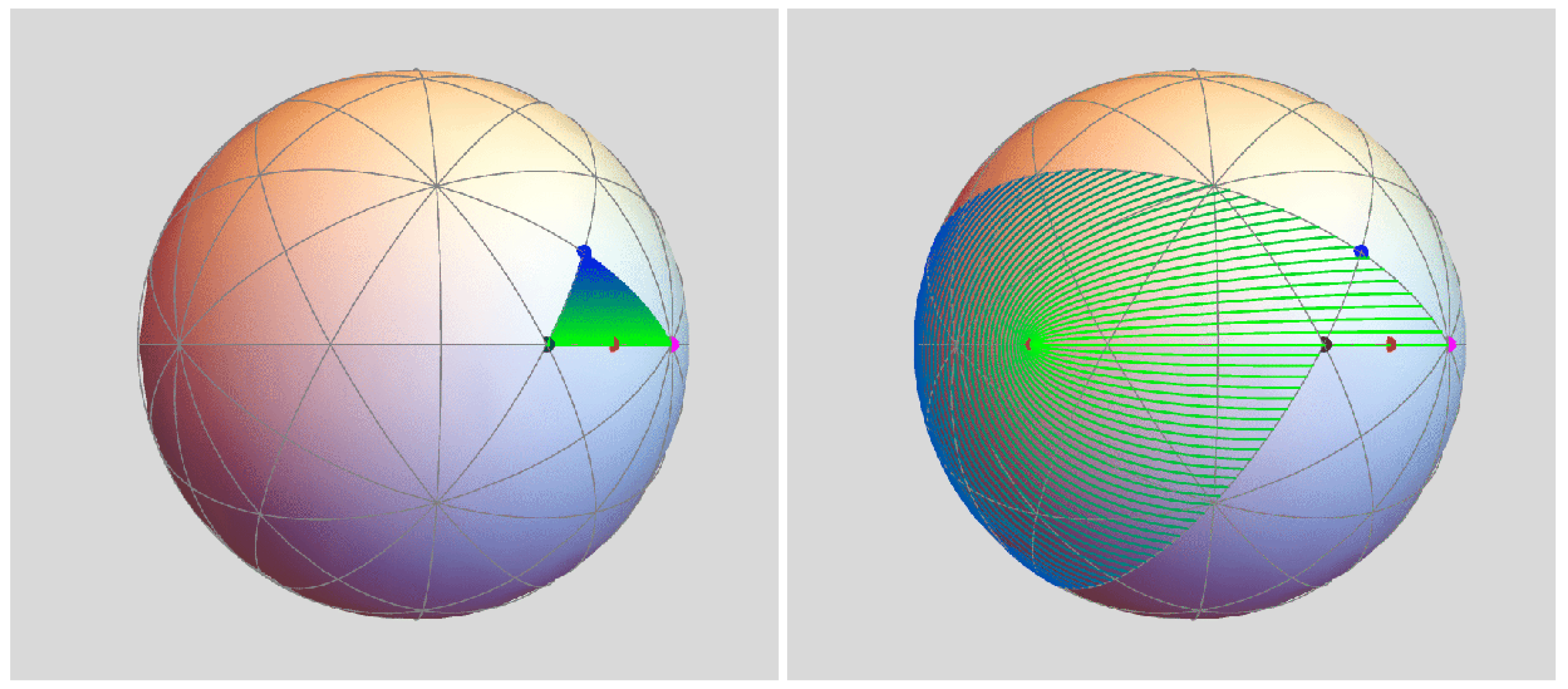
Realizing the structure of a spherical polyhedron requires a system of edges between critical points that appears naturally from a map’s behavior. Serving as an archetype is the soccer ball map where the collection of edges is a forward invariant set in which the image of a single face K is a union of faces that are canonically associated with K—namely, the complement of K’s antipodal face.

7.1. Constructing Edges

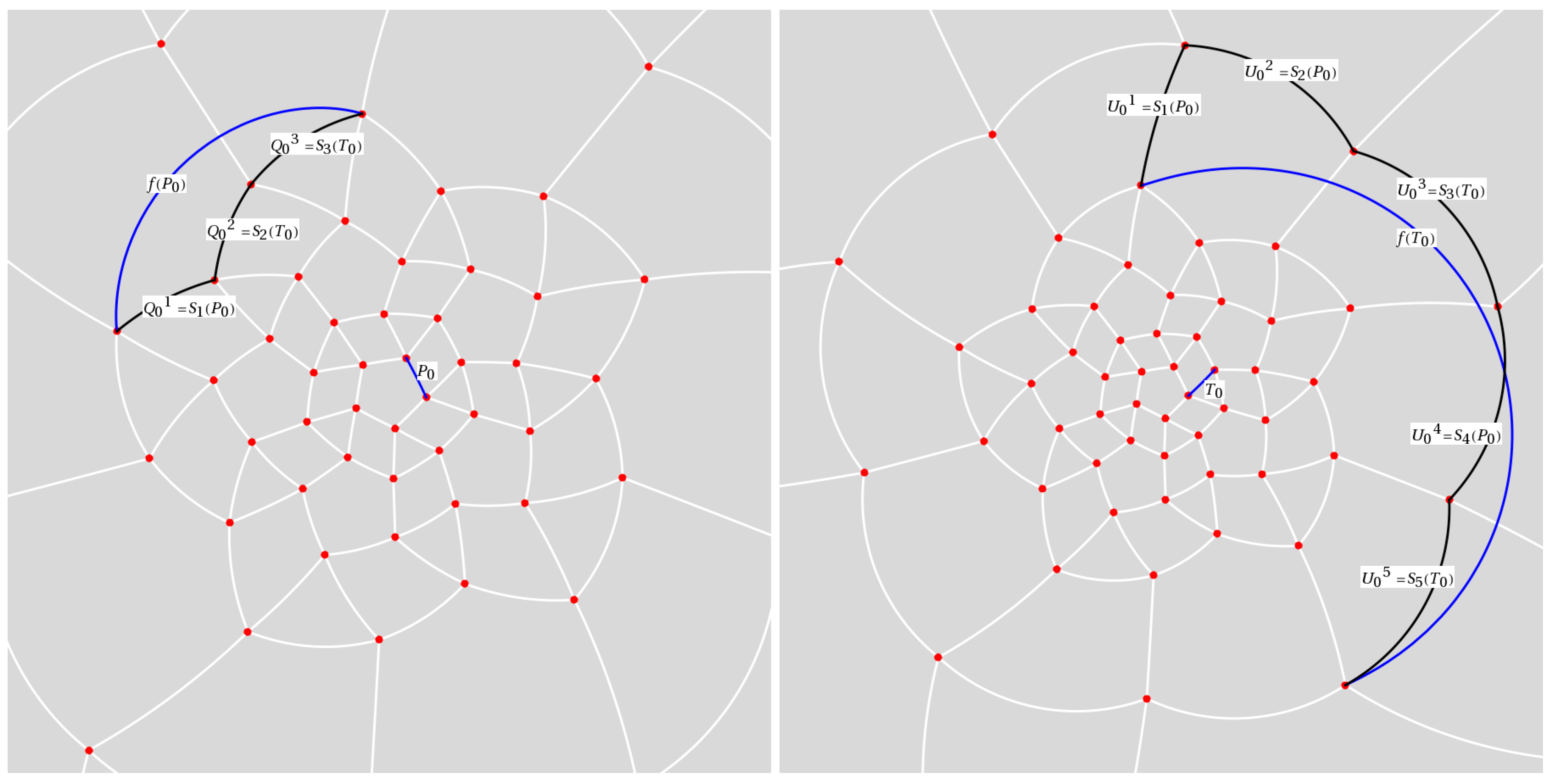
What follows is a fairly elaborate description of a method that, for a 31-map f, constructs edges between adjacent vertices (periodic critical points). Working on the sphere, adjacency is determined by triangular and pentagonal arrangements of critical points nearest to 3-fold and 5-fold axes. In every case, a common heuristic element first connects adjacent vertices by a great-circle arc. Given such a “proto-edge” T 0 or P 0 (depending upon whether the arc spans adjacent triangular vertices ( t 1 , t 2 ) or pentagonal vertices ( p 1 , p 2 ) , we use the image f ( T 0 ) or f ( P 0 ) to indicate a collection of edges to which an actual edge maps. To be specific, say that we’re approximating an actual pentagonal edge P that spans ( p 1 , p 2 ) —illustrated in Figure 5. The procedure generates the actual edge as a result of an infinite number of iterative steps.
The first step identifies an ordered set of B 62 vertices
( v 0 = f ( p 1 ) ,     , v k ,     , v m = f ( p 2 ) )
through which f ( P ) is to pass. Given an adjacent pair of triangular vertices ( v k 1 , v k ) , there’s a unique element S k I such that either
( S k ( t 1 ) , S k ( t 2 ) ) = ( v k 1 , v k ) or ( S k ( t 2 ) , S k ( t 1 ) ) = ( v k 1 , v k ) .
Similarly, if ( v k 1 , v k ) is an adjacent pair of pentagonal vertices, a unique S k I satisfies either
( S k ( p 1 ) , S k ( p 2 ) ) = ( v k 1 , v k ) or ( S k ( p 2 ) , S k ( p 1 ) ) = ( v k 1 , v k ) .
Connect ( v k 1 , v k ) by the appropriate “pushed” proto-edge Q 0 k = S k ( X k ) , where X k is either P 0 or T 0 . Every ( v k 1 , v k ) in ( v 0 , , v m ) is now spanned by great circle arcs.
In order to approximate a triangular edge T, the technique gives pushed edges
( U 0 1 = Z 1 ( Y 1 ) ,     , U 0 n = Z n ( Y n ) ) ,
where Z k I is the analogue of S k and Y k is either P 0 or T 0 . Comparing the pushed paths ( Q 0 1 , , Q 0 m ) and ( U 0 1 , , U 0 n ) to the respective images f ( P 0 ) and f ( T 0 ) reveals their homotopic equivalence, as Figure 5 illustrates in the plane.
There’s a degree of freedom in choosing the endpoints of the Q 0 k and U 0 k . Here, we select endpoints so that a map’s geometric description respects “P-caps”—a pentagonal face with its surrounding five triangles and five quadrilaterals. Figure 6 shows a schematic P-cap in a planar B 62 structure.
In step two, we use suitable branches of f 1 to pull back the pushed segments ( Q 0 1 , , Q 0 m ) to a first generation edge P 1 between ( p 1 , p 2 ) . In practice, this is accomplished as follows:
  • Select equally-spaced points ( b k 1 , , b k n k ) along each Q 0 k .
  • Compute the elements in f 1 ( b k ) for = 1 , , n k .
  • Extract from f 1 ( b k ) the inverse image points ( a k 1 , , a k n k ) that minimize the sum of the distances to p 1 and p 2 .
  • Taylor expand f about a k for = 1 , , n k .
  • Obtain the desired single-valued branch γ k of f 1 by inverting the Taylor series for f at a k . The choice of branch yields
    γ k ( b k ) = a k .
  • Compute the “pulled” segmented paths that span ( p 1 , p 2 ) :
    P 1 1 =   γ 1 1 ( Q 0 1 ) ,     , γ 1 n 1 ( Q 0 1 ) P 1 m =   γ m 1 ( Q 0 m ) ,     , γ m n m ( Q 0 m ) .
Notice that, in a pulled segment, different branches of the inverse map are applied to the same parametrized segment Q 0 k . We arrive at the appropriate pulled segment by selecting a subinterval of the parameter interval. In the triangular case, we get first-generation pulled edges ( T 1 1 , , T 1 n ) .
Step three begins an iteration of the process by moving the pulled segments to the pushed locations:
Q 1 1 , 1 = S 1 ( X 1 1 ) , Q 1 1 , 2 = S 1 ( X 1 2 ) ,     , Q 1 m , m = S m ( X 1 m )
and
U 1 1 , 1 = Z 1 ( Y 1 1 ) , U 1 1 , 2 = Z 1 ( Y 1 2 ) ,     , U 1 n , n = Z n ( Y 1 n ) ,
where X 1 k and Y 1 k are either P 1 k or T 1 k . Observe that the subscript of P, Q, T, and U is the generation number. The group elements S k and Z k act on each component of the respective X 1 k or Y 1 k . For example,
Q 1 k , = S k ( P 1 ) =   S k ( γ k 1 ( Q 0 ) ) ,     , S k ( γ k n k ( Q 0 ) ) .
Applying the push transformations S k to the centers of Taylor expansion a r produces a fresh set of points
b k , 1 = S k ( a 1 ) ,     , b k , n k = S k ( a n k )
on the pushed segments Q 1 k , . Inverse images of the b k , i then become a new set of Taylor centers a k , i with associated branches γ k , i of f 1 .
Next, the fourth step constructs second-generation segments at ( p 1 , p 2 ) and ( t 1 , t 2 ) by pulling back the pushed edges. For a pentagonal edge,
P 2 k , = γ k , 1 ( Q 1 k , ) ,     , γ k , n k ( Q 1 k , ) .
The second-generation approximation of P is the collection of segments
( P 2 1 , 1 ,     , P 2 1 , n 1 ) ,     , ( P 2 m , 1 ,     , P 2 m , n m ) .
As before, when the second-generation segments are pushed and then pulled, the group elements distribute over components, whereas the components distribute over the branches of f 1 .
Letting the number of iterations of the push–pull algorithm grow without bound, the edge P emerges:
( k i ) γ k r + 1 k r , , k 1 S k r + 1 γ k r k r 1 , , k 1 S k r γ k 2 k 1 S k 2 ( P 0 ) = P ,
where ( k i ) ranges over all permissible sequences. Grouping the push–pull action as γ     S produces a set that spans the endpoints of P 0 . A similar dynamic yields a triangular edge T.
Evidently, for a selected ( k i ) , the procedure converges due to the collection
γ k r k r 1 , , k 1 S k r
being a normal family ([2], Theorem 9.2.1). In more geometric terms, under f, a proto-edge undergoes a net expansion. As exemplified in Figure 5, P 0 experiences roughly a three-fold stretch and T 0 expands approximately by a factor of five. The expanding behavior occurs on the complement of a neighborhood of the superattracting periodic points. When pulled back, the pieces of the pushed proto-edges that are bounded away from the critical points undergo a net contraction reciprocal to the expansion under forward iteration. In each push–pull cycle, this contraction occurs away from points in the pre-critical set k f k ( C f ) , while the push transformation is a spherical isometry. The iterative effect of this contraction is clustering among the pulled-back points.
With P and T in hand, the icosahedral action produces a system of edges for a dynamical polyhedron: E f = I ( P )     I ( T ) . Graphical constructions of second-generation approximations for the 31-maps appear in the following section. This construction satisfies a key property of a dynamical polyhedron.
Proposition 2.
The system of edges E f is forward invariant under f.
Proof. 
The push–pull construction of P iterates the map γ S where, for ease of description, indices are suppressed. That is,
( γ S ) r ( P 0 ) r A P .
(Since the γ maps are local inverses of f, the limit set A is only contained in P.) Applying f gives
f ( γ S ) r ( P 0 ) r f ( A ) f ( γ S ) ( γ S ) r 1 ( P 0 ) r f ( A ) ( f γ ) S ( γ S ) r 1 ( P 0 ) r f ( A ) S ( γ S ) r 1 ( P 0 ) r f ( A ) .
Since
S ( γ S ) r 1 ( P 0 ) r S ( A ) ,
f ( A ) = S ( A ) I ( P ) . Of course, a similar result holds for a triangular edge T. □
Worth noting here is that we can view a dynamical polyhedron as a graph on the sphere or plane that covers itself under its associated map. As such, the B 62 geometry of a graph determined by a 31-map would appear to be non-hyperbolic [10].

7.2. Combinatorial Classification

Here, we’ll treat the behavior of the 56 maps that result from solving the parameter equations P 12 = 0 , P 20 = 0 , and P 24 = 0 . For a map f, the computational graphics displayed in Section 8 solves a combinatorial problem: Given a face A of f’s polyhedron, what collection of faces does f ( A ) cover?
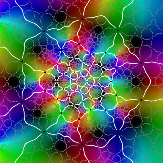
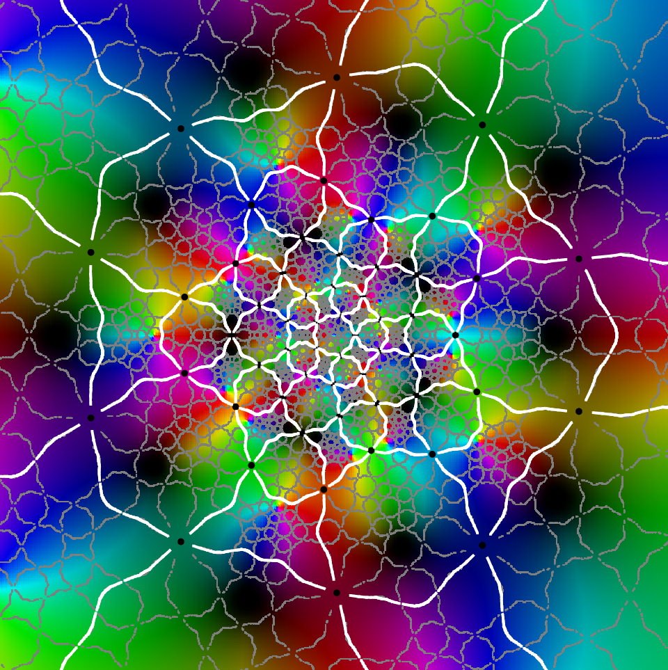
Referring to the graphical results, the second-generation system of edges E f appears in white. (Note the change in usage: here, E f refers to an approximation of the actual system of edges.) Gaps around the critical points are due to the large expansion under the pullback. Given a point z 0 on an edge, we pull back to f 1 ( z 0 ) by solving f ( z ) = z 0 . In the plot on the left side, the gray curves correspond to the inverse image f 1 ( E f ) . The pulled-back edges reveal the beginnings of a fractal structure: within each face A, there is a collection of “pre-faces” that indicates what face-types f ( A ) covers. Note that E f is close to being a subset of f 1 ( E f ) —visual evidence that E f is approximately f-invariant.
Using a map-coloring procedure, we can discern which faces f ( A ) covers. Given a map f ( z ) on C , define color functions for hue and luminosity
H f ( z ) = Arg ( f ( z ) ) 2   π and L f ( z ) = 2 | f ( z ) | ,
where Arg ( z ) [ 0 , 2   π ] is a branch of the argument taken modulo 2   π . Each function takes on values in [ 0 , 1 ] with hue varying from blue to green and luminosity from bright to dark.
The plots on the right show E f overlaid on a reference coloring for the identity map I. On the left, we see the pulled-back faces on top of the coloring for a 31-map f. By matching the color properties of a pre-face on the left with those of a face on the right, we can determine which face turns out to be its image. That is, f ( z ) = w when
( H f ( z ) , L f ( z ) ) = ( H I ( w ) , L I ( w ) ) .
For instance, the point at infinity is the center of a pentagonal face P . As a consequence, | f ( z ) | is large and dark pentagonal pre-faces cover P .
The maps are classified according to their combinatorial and topological descriptions. Pullback structures within a class are topologically equivalent.
By way of illustrating the combinatorics and topology, we consider the map g introduced previously. Its critical set realizes an achiral B 62 configuration whereby the critical points lie on the mirrors of reflective icosahedral symmetry. As is the case for all of the 31-maps, the centers of a pentagon and triangle are fixed by g while a quadrilateral’s center is sent to its antipode.
The geometric behavior of g differs from that of the two soccer ball maps—which are not included here since their dynamical polyhedra do not have B 62 structure and they have been considered elsewhere. A face does not map to the complement of an antipodal face, as that would require the degree to be 61. Computational graphics (plots at the top of Class I) reveal that g wraps a face onto a union of P-caps that is icosahedrally associated with the face. The image of a pentagonal face P covers the cap to which it belongs as well as the five caps that intersect P’s cap. For a triangular face T, g ( T ) covers the three caps whose intersection includes T. Finally, the image of a quadrilateral Q covers the complement of four P-caps two of which intersect Q while the other two caps intersect the former two caps.
Using its geometric description, we can work out g’s topological degree by counting inverse images. The relevant data are recorded in Table 1 as the number of faces of each type that belong to the g-image of a given face-type. For instance, the first row reports that a pentagon maps to six caps the union of which contains six pentagons, fifteen triangles, and twenty quadrilaterals.
The number of times a pentagonal face is covered equals the total number of pentagons that appear as images of faces divided by the number of pentagonal faces. Reading down the P column,
12 · 6 + 20 · 3 + 30 · 8 12 = 31 .
Similar treatment of triangular and quadrilateral faces yields the number of faces in the inverse image of the respective face:
12 · 15 + 20 · 10 + 30 · 8 20 = 12 · 20 + 20 · 12 + 30 · 15 30 = 31 .
The gallery of plots places the maps into combinatorial classes, with three exceptions. Each class has a complementary class for which the topological description replaces “n P-caps about X” by “complement of n P-caps about X ˜ ” and “complement of n P-caps about X” by “n P-caps about X ˜ ” where X ˜ is the antipode of X. Of course, a chiral map f and its heterochiral partner f ¯ (not shown) belong to the same class.

8. Periodic Table

Table 2, Table 3, Table 4, Table 5, Table 6, Table 7, Table 8, Table 9, Table 10, Table 11, Table 12, Table 13 and Table 14 record the combinatorial data regarding the covering behavior of each class of maps.
Class I
P   six   P -caps   about   P T   three   P -caps   about   T Q   complement   of   four   P -caps   about   Q
Symmetry 12 00177 i001 Symmetry 12 00177 i002
the map g discussed in Section 6period 2, achiral
Symmetry 12 00177 i003 Symmetry 12 00177 i004
period 3
Symmetry 12 00177 i005 Symmetry 12 00177 i006
period 5
Symmetry 12 00177 i007 Symmetry 12 00177 i008
period 5
Class Ic
P   complement   of   six   P -caps   about   P ˜ T   complement   of   three   P -caps   about   T ˜ Q   four   P -caps   about   Q ˜
Symmetry 12 00177 i009 Symmetry 12 00177 i010
the map h discussed in Section 6period 2, achiral
Symmetry 12 00177 i011 Symmetry 12 00177 i012
period 2
Symmetry 12 00177 i013 Symmetry 12 00177 i014
period 3
Symmetry 12 00177 i015 Symmetry 12 00177 i016
period 3
Class II
P   one   P -cap   about   P T   three   P -caps   about   T Q   complement   of   two   P -caps   about   Q
Symmetry 12 00177 i017 Symmetry 12 00177 i018
period 3
Symmetry 12 00177 i019 Symmetry 12 00177 i020
period 5
Symmetry 12 00177 i021 Symmetry 12 00177 i022
period 5
Class IIc
P   complement   of   one   P -cap   about   P ˜ T   complement   of   three   P -caps   about   T ˜ Q   two   P -caps   about   Q ˜
Symmetry 12 00177 i023 Symmetry 12 00177 i024
period 3
Symmetry 12 00177 i025 Symmetry 12 00177 i026
period 3
Symmetry 12 00177 i027 Symmetry 12 00177 i028
period 5
Class III
P   six   P -caps   about   P T   nine   P -caps   about   T Q   complement   of   eight   P -caps   about   Q
Symmetry 12 00177 i029 Symmetry 12 00177 i030
period 3
Symmetry 12 00177 i031 Symmetry 12 00177 i032
period 3
Symmetry 12 00177 i033 Symmetry 12 00177 i034
period 5
Class IIIc
P   complement   of   six   P -cap   about   P ˜ T   complement   of   nine   P -caps   about   T ˜ Q   eight   P -caps   about   Q ˜
Symmetry 12 00177 i035 Symmetry 12 00177 i036
period 3
Symmetry 12 00177 i037 Symmetry 12 00177 i038
period 5
Symmetry 12 00177 i039 Symmetry 12 00177 i040
period 5
Class IV
P   P = complement   of   11   P -caps   about   P ˜ T   complement   of   nine   P -caps   about   T ˜ Q   ten   P -caps   about   Q ˜
Symmetry 12 00177 i041 Symmetry 12 00177 i042
period 5
Symmetry 12 00177 i043 Symmetry 12 00177 i044
period 5
Class IVc
P   complement   of   P ˜ = 11   P -caps   about   P T   nine   P -caps   about   T Q   complement   of   ten   P -caps   about   Q
Symmetry 12 00177 i045 Symmetry 12 00177 i046
period 2
Class V
P   one   P -cap   about   P T   complement   of   nine   P -caps   about   T ˜ Q   complement   of   7 -block   about   Q   ( 7 -block = Q -cap 2 · Q )
Symmetry 12 00177 i047 Symmetry 12 00177 i048
period 2
Class Vc
P   complement   of   one   P -cap   about   P ˜ T   nine   P -caps   about   T Q   7 -block   about   Q ˜
Symmetry 12 00177 i049 Symmetry 12 00177 i050
period 5
Exceptional cases
P   six   P -caps   about   P T   complement   of   three   P -caps   at   T ˜ Q   two   P -caps     2 · P   2 · Q   about   Q ˜
Symmetry 12 00177 i051 Symmetry 12 00177 i052
period 2
Exceptional cases
P   six   P -caps   about   P T   complement   of   three   P -caps   at   T ˜ Q   two   P -caps     2 · P   2 · Q   about   Q ˜
Symmetry 12 00177 i053 Symmetry 12 00177 i054
period 2
P   one   P -cap   about   P T   T Q   18   T -caps   about   Q ˜   ( complement   of   Q 2 · T )
Symmetry 12 00177 i055 Symmetry 12 00177 i056
period 3
P   complement   of   six   P -caps   about   P ˜ T   complement   of   six   P -caps   about   T ˜ Q   six   P -caps   about   Q ˜
Symmetry 12 00177 i057 Symmetry 12 00177 i058
period 5

Funding

This research received no external funding.

Acknowledgments

The work represented in this article grew out of discussions with Peter Doyle to whom I owe a large debt of gratitude. I thank the referees for comments and the references [9,10].

Conflicts of Interest

The author declares no conflict of interest.

References

  1. Doyle, P.; McMullen, C. Solving the quintic by iteration. Acta Math. 1989, 163, 151–180. [Google Scholar] [CrossRef]
  2. Beardon, A. Iteration of Rational Functions; Springer: Berlin/Heidelberg, Germany, 1991. [Google Scholar]
  3. Crass, S. Dynamics of a soccer ball. Exp. Math. 2014, 23, 261–270. [Google Scholar] [CrossRef]
  4. Crass, S. Available online: www.csulb.edu/~scrass/math.html (accessed on 1 January 2020).
  5. Klein, F. Lectures on the Icosahedron; Dover Books: New York, NY, USA, 1956. [Google Scholar]
  6. Douady, A.; Hubbard, J. A proof of Thurston’s topological characterization of rational functions. Acta Math. 1993, 171, 263–297. [Google Scholar] [CrossRef]
  7. Thurston, D. Elastic graphs. Forum Math. Sigma 2019, 7, e24. [Google Scholar] [CrossRef] [Green Version]
  8. Thurston, D. A positive characterization of rational maps. arXiv 2016, arXiv:1612.04424. [Google Scholar]
  9. Shang, Y. A combinatorial necessary and sufficient condition for cluster consensus. Neurocomputing 2016, 216, 611–616. [Google Scholar] [CrossRef]
  10. Shang, Y. Lack of Gromov-hyperbolicity in small-world networks. Open Math. 2012, 10, 1152–1158. [Google Scholar] [CrossRef]
Figure 1. Schematic B 62 labeled for period-2 behavior.
Symmetry 12 00177 g001
Figure 2. Achiral critical sets of g (red) and h (blue).
Symmetry 12 00177 g002
Figure 3. Fundamental triangle and its image under g: On the left, we see the collection of 120 triangles into which the sphere is carved by the 15 lines of reflective icosahedral symmetry. One such 235 triangle is filled with line segments parallel to the hypotenuse and having a color gradient running perpendicular to the hypotenuse. Any one of the 235 triangles is fundamental relative to the extended icosahedral action I ˜ . That is, applying the elements of I ˜ to the triangle will tile the sphere as the plot shows. The image on the right plots the result of applying g to each of the segments in the shaded triangle on the left. Exactly 31 of the 235 triangles are covered by the image—thus revealing g’s topological and algebraic degrees.
Symmetry 12 00177 g003
Figure 4. Fundamental triangle and its image under h.
Symmetry 12 00177 g004
Figure 5. Homotopy between select proto-edges and the image of a proto-edge for a pentagon (left) and a triangle (right) in a B 62 under one of the 31-maps f. The images of the proto-edges P 0 and T 0 (blue arcs) are respectively homotopic to a chain of pushed versions of P 0 and T 0 (black arcs). In this sample, the pushed edges associated with f ( P 0 ) are PPT (pentagon–pentagon–triangle) starting with f ( p 1 ) while those associated with f ( T 0 ) are PPTPT beginning at f ( t 1 ) .
Symmetry 12 00177 g005
Figure 6. A P-cap in a B 62 .
Symmetry 12 00177 g006
Table 1. Images of faces under g.
PTQ
P61520
T31012
Q8815
Table 2. Class I.
Table 2. Class I.
PTQ a · X Total Number of Times X Faces Are Covered
P61520 12 · P 12 · 6 + 20 · 3 + 30 · 8 = 12 · 31
T31012 20 · T 12 · 15 + 20 · 10 + 30 · 8 = 20 · 31
Q8815 30 · Q 12 · 20 + 20 · 12 + 30 · 15 = 30 · 31
Table 3. Class Ic.
Table 3. Class Ic.
PTQ a · X Total Number of Times X Faces Are Covered
P6510 12 · P 12 · 6 + 20 · 9 + 30 · 4 = 12 · 31
T91018 20 · T 12 · 5 + 20 · 10 + 30 · 12 = 20 · 31
Q41215 30 · Q 12 · 10 + 20 · 18 + 30 · 15 = 30 · 31
Table 4. Class II.
Table 4. Class II.
PTQ a · X Total Number of Times X Faces Are Covered
P155 12 · P 12 · 1 + 20 · 3 + 30 · 10 = 12 · 31
T31012 20 · T 12 · 5 + 20 · 10 + 30 · 12 = 20 · 31
Q101221 30 · Q 12 · 5 + 20 · 12 + 30 · 21 = 30 · 31
Table 5. Class IIc.
Table 5. Class IIc.
PTQ a · X Total Number of Times X Faces Are Covered
P111525 12 · P 12 · 11 + 20 · 9 + 30 · 2 = 12 · 31
T91018 20 · T 12 · 15 + 20 · 10 + 30 · 8 = 20 · 31
Q289 30 · Q 12 · 25 + 20 · 18 + 30 · 9 = 30 · 31
Table 6. Class III.
Table 6. Class III.
PTQ a · X Total Number of Times X Faces Are Covered
P61520 12 · P 12 · 6 + 20 · 9 + 30 · 4 = 12 · 31
T91927 20 · T 12 · 15 + 20 · 19 + 30 · 2 = 20 · 31
Q425 30 · Q 12 · 20 + 20 · 27 + 30 · 5 = 30 · 31
Table 7. Class IIIc.
PTQ a · X Total Number of Times X Faces Are Covered
P6510 12 · P 12 · 6 + 20 · 3 + 30 · 8 = 12 · 31
T313 20 · T 12 · 5 + 20 · 1 + 30 · 18 = 20 · 31
Q81825 30 · Q 12 · 10 + 20 · 3 + 30 · 25 = 30 · 31
Table 8. Class IV.
Table 8. Class IV.
PTQ a · X Total Number of Times X Faces Are Covered
P100 12 · P 12 · 1 + 20 · 3 + 30 · 10 = 12 · 31
T313 20 · T 12 · 0 + 20 · 1 + 30 · 20 = 20 · 31
Q102029 30 · Q 12 · 0 + 20 · 3 + 30 · 29 = 30 · 31
Table 9. Class IVc.
Table 9. Class IVc.
PTQ a · X Total Number of Times X Faces Are Covered
P112030 12 · P 12 · 11 + 20 · 9 + 30 · 2 = 12 · 31
T91927 20 · T 12 · 20 + 20 · 19 + 30 · 0 = 20 · 31
Q201 30 · Q 12 · 30 + 20 · 27 + 30 · 1 = 30 · 31
Table 10. Class V.
Table 10. Class V.
PTQ a · X Total Number of Times X Faces Are Covered
P155 12 · P 12 · 1 + 20 · 3 + 30 · 10 = 12 · 31
T313 20 · T 12 · 5 + 20 · 1 + 30 · 18 = 20 · 31
Q101827 30 · Q 12 · 5 + 20 · 3 + 30 · 27 = 30 · 31
Table 11. Class Vc.
Table 11. Class Vc.
PTQ a · X Total Number of Times X Faces Are Covered
P111525 12 · P 12 · 11 + 20 · 9 + 30 · 2 = 12 · 31
T91927 20 · T 12 · 15 + 20 · 19 + 30 · 2 = 20 · 31
Q223 30 · Q 12 · 25 + 20 · 27 + 30 · 3 = 30 · 31
Table 12. Exceptional case.
PTQ a · X Total Number of Times X Faces Are Covered
P61520 12 · P 12 · 6 + 20 · 9 + 30 · 4 = 12 · 31
T91018 20 · T 12 · 15 + 20 · 10 + 30 · 8 = 20 · 31
Q4811 30 · Q 12 · 20 + 20 · 18 + 30 · 11 = 30 · 31
Table 13. Exceptional case.
PTQ a · X Total Number of Times X Faces Are Covered
P155 12 · P 12 · 1 + 20 · 0 + 30 · 12 = 12 · 31
T010 20 · T 12 · 5 + 20 · 1 + 30 · 18 = 20 · 31
Q121829 30 · Q 12 · 5 + 20 · 0 + 30 · 29 = 30 · 31
Table 14. Exceptional case.
PTQ a · X Total Number of Times X Faces Are Covered
P6510 12 · P 12 · 6 + 20 · 6 + 30 · 6 = 12 · 31
T649 20 · T 12 · 5 + 20 · 4 + 30 · 16 = 20 · 31
Q61621 30 · Q 12 · 10 + 20 · 9 + 30 · 21 = 30 · 31

