Co-Training Semi-Supervised Deep Learning for Sentiment Classification of MOOC Forum Posts


1
School of Information Science and Technology, Northwest University, Xi’an 710127, Shaanxi, China
2
State-Province Joint Engineering and Research Center of Advanced Networking and Intelligent Information Services, School of Information Science and Technology, Northwest University, Xi’an 710127, Shaanxi, China
*
Author to whom correspondence should be addressed.
Symmetry 2020, 12(1), 8; https://doi.org/10.3390/sym12010008
Submission received: 16 November 2019
/
Revised: 11 December 2019
/
Accepted: 13 December 2019
/
Published: 18 December 2019
Abstract
:Sentiment classification of forum posts of massive open online courses is essential for educators to make interventions and for instructors to improve learning performance. Lacking monitoring on learners’ sentiments may lead to high dropout rates of courses. Recently, deep learning has emerged as an outstanding machine learning technique for sentiment classification, which extracts complex features automatically with rich representation capabilities. However, deep neural networks always rely on a large amount of labeled data for supervised training. Constructing large-scale labeled training datasets for sentiment classification is very laborious and time consuming. To address this problem, this paper proposes a co-training, semi-supervised deep learning model for sentiment classification, leveraging limited labeled data and massive unlabeled data simultaneously to achieve performance comparable to those methods trained on massive labeled data. To satisfy the condition of two views of co-training, we encoded texts into vectors from views of word embedding and character-based embedding independently, considering words’ external and internal information. To promote the classification performance with limited data, we propose a double-check strategy sample selection method to select samples with high confidence to augment the training set iteratively. In addition, we propose a mixed loss function both considering the labeled data with asymmetric and unlabeled data. Our proposed method achieved a 89.73% average accuracy and an 93.55% average F1-score, about 2.77% and 3.2% higher than baseline methods. Experimental results demonstrate the effectiveness of the proposed model trained on limited labeled data, which performs much better than those trained on massive labeled data.
1. Introduction
As a key form of online education, massive open online courses (MOOCs) have gained tremendous popularity. The number of enrolled participants increased from eight million in 2013 to 101 million in 2018 [1,2]. MOOC discussion forums provide a fertile ground for learners to post freely online about their personal learning experiences, feelings, and viewpoints [3,4]. Sentiment classification of those valuable forum posts can assist instructors to make interventions and guiding instructions to improve learning performance. Lacking monitoring on learners’ sentiments may lead to high dropout rates of courses [5]. Moreover, the forum posts may contain significant sentiment orientation for institutions to incorporate changes to improve their course quality, teaching strategies, and other academic elements [6].
Sentiment classification aims to classify forum posts containing personal mind-sets into several categories, such as negative, positive, favorable, unfavorable, thumbs up, thumbs down [7]. Generally, learners generate a large volume of forum posts, even tens of thousands of forum posts for one course. Due to the very high learner-to-instructor ratios in online learning environment, it is unrealistic to expect instructors to fully track the forum posts to identify learners’ sentiment orientations and provide feedback in a timely manner [8]. Thus, it is necessary to use machine learning techniques to complete sentiment classification.
Most recently, deep learning has emerged as an outstanding machine learning technique with a great potential for sentiment classification [9,10,11]. Instead of depending on manually-engineered shallow features, deep learning methods make complex feature extraction automatically and have richer representation capabilities [12]. Despite such attractiveness, deep neural networks always rely on a large amount of labeled data for supervised training; e.g., IMDB with 50,000 labeled posts. In many real-world applications, the amount of labeled data is very small compared to that of unlabeled data. Moreover, labeling a large amount of data is expensive and time consuming [13].
Semi-supervised deep learning combines supervised deep learning and unsupervised deep learning, utilizing a small amount of labeled data and a large amount of unlabeled data simultaneously to train the model [14]. Roughly speaking, existing semi-supervised learning methods are classified into several categories, including generative approaches, semi-supervised support vector machines, graph-based approaches, and discrimination-based approaches [15]. A key part of discrimination-based approaches is to generate multiple classifiers, including combining different views with a single classifier, or combining a single view with different classifiers. Compared to other methods, discrimination-based approaches pay more attention to views, which can be considered text representations in the sentiment classification of MOOC forum posts.
Better text representation is a prerequisite to achieving good results in sentiment classification of MOOC forum posts [16]. Word and character-based embedding are two mainstream techniques for text representations in many NLP tasks [17], both representing words as low-dimensional vectors. The embedding representation is able to reveal hidden semantic relationships between words and support capturing the contextual similarities of words due to the numerical representation learning from the context information. Some studies use a single view or concatenate vectors of the two views (word embedding and character-based embedding) [18,19]. Nevertheless, when few training data are available and high classification accuracy is expected to achieve, the strategy is not comprehensive because the training samples may not describe the data distribution adequately from either the view of word embedding or character-based embedding.
As an important paradigm of the discrimination-based semi-supervised algorithm, co-training requires that two views have historically been proven to be effective for sentiment classification when there are only limited labeled data and massive unlabeled data [20,21]. Moreover, Blum et al. have given theoretical proofs to guarantee the success of co-training in utilizing the unlabeled data [22]. Thus, this paper applies co-training to sentiment classification of MOOC forum posts, taking advantage of the two views of word-based and character-based representations.
Co-training is a semi-supervised learning technique which trains two classifiers based on two different views of data [23]. It assumes that each sample is described based on two different feature views that provide different, complementary information about the sample. Ideally, the two views are independent and each view is sufficient, such that the class of a sample can be accurately predicted from each view alone. Co-training first learns a separate classifier for each view using a small amount of labeled data. Then, the samples with the most confident predictions of each classifier on the unlabeled data are added to the labeled data iteratively.
In the two views of co-training in this paper, we represent a word as vectors based on word embedding and character-based embedding independently because of their successful applications in sentiment analysis. Word embedding algorithms take a word as a basic unit and dense, real-valued representations of words as low dimensional vectors. In order to obtain high quality vector space representations for sentiment classification of MOOC posts, it is necessary to use a large number of texts in the educational field as training data. Unfortunately, it always takes too much time to train word vectors from a large-scale corpus. Nevertheless, there are many pretrained word vectors which are freely available and of high quality. Thus, on the one hand, we directly utilize the pretrained word vectors as one view of co-training, which takes advantage of large-scale corpus and considers context between words.
Simply relying on pretrained word vectors alone does not accurately express the contextual meaning of a word because the word may have different meanings in different contexts and the word vectors are static so will not change in different contexts. Moreover, the internal information of a word is also related to the meaning of each of its characters. Character-based embedding algorithms take a character as a basic unit and dense, real-valued representations of words as low dimensional vectors. Compared to word embedding, character-based embedding captures the information about the word morphology and internal structures of words and targets toward a particular domain. Moreover, it can generate word vectors according to the context, which takes advantage of task-specific corpus. Thus, on the other hand, we take character-based embedding as another view of co-training.
One key to the success of co-training lies in how to select confident samples from the unlabeled samples to augment the training set [24,25]. Previous studies use various sample selection strategies, such as using the classifier’s posteriori probability as the labeling confidence metric [22], ten-fold cross validation on the original labeled set [26], and ensemble learning [23]. Nevertheless, those methods select samples from unlabeled data only from the perspective of training set or classifiers, which may fail to obtain high confident samples. To address this problem, inspired by ensemble learning and the text characteristic of high similarity of a training set in one class, we propose a novel, double-check strategy sample selection method both considering the perspective of classifiers and the training set, respectively.
Another key issue of boosting the performance of semi-supervised learning is to define a loss function that handles both labeled and unlabeled data. A few studies have proposed the appropriate mixed loss functions of cross-entropy, entropy minimization, etc., trying to improve the classification performance of semi-supervised learning [27,28,29]. Nevertheless, current studies ignore the problem of imbalanced data distributions existing in many datasets [30]. Thus, to achieve accurate sentiment classification, we propose a mixed loss function for semi-supervised learning both handling imbalanced labeled data and unlabeled data.
Generally, the goal of this paper is to explore how to utilize limited labeled data and massive unlabeled data to construct a model with performance comparable to those trained on massive labeled data. The major contributions of this paper can be summarized as follows: (1) We propose a co-training semi-supervised model, which captures the external and internal information from word embedding and character-based embedding, taking advantage of a large-scale and task-specific corpus. (2) We propose a double-check strategy sample selection method to obtain reliable estimates of either classifiers’ labeling confidence on unlabeled examples, aiming to boost the classification performance of co-training iteratively with limited labeled data. (3) We propose a mixed loss function for the proposed deep semi-supervised model, both considering the distribution characteristic of imbalanced labeled and unlabeled data.
2. Related Work
2.1. Sentiment Classification of MOOC Forum Posts
Traditional supervised learning. Sentiment classification has been highlighted as a key issue and catalyzed much research in online educational environments. A substantial number of initial approaches utilize lexicon-based methods [31]. A sentiment lexicon is constructed necessarily by a list of lexical features labeled according to the semantic orientation [32]. Kaewyong et al. proposed to investigate learners’ free style text comments to predict teacher performance based on lexicon sentiment classification [33]. One comment was classified into positive and negative according to its overall sentiment orientation. To monitor learners’ trending opinions in MOOC learning, Wen et al. explored to mine course-level and user-level sentiment based on lexicon of texts from forum posts [34]. The two works had the limitation that they both utilized the manually designed lexicon.
Since it is complicated to construct a comprehensive sentiment lexicon, much attention has been focused on automatic identification of sentiment using features by various machine learning approaches [35,36,37]. These typical features for sentiment including bag-of-words (BOW), n-grams, and TF-IDF [38]. The traditional surface machine learning approaches face two challenges. The first one is that the methods heavily rely on feature engineering which needs complex, manually extracted features. The second one is that they need a large number of labeled data for supervised learning to train models.
Deep supervised learning. In contrast with feature-based machine learning methods, a deep neural network can extract features automatically and has stronger representation capabilities. There are two main deep neural network architectures: the convolutional neural network (CNN) and the recurrent neural network. Long short-term memory (LSTM) and the gated recurrent unit were developed to alleviate the limitation of vanishing gradient of the basic recurrent neural network. For example, Nguyen et al. applied a deep CNN to course-level prediction based on forum posts for correct recognition of instances of the minority class which included learners with failing grades [39]. Ramón et al. utilized a CNN to detect the positive or negative polarity of learners’ opinions regarding the exercises they solved in an intelligent learning environment [6]. Wei et al. proposed a transfer learning framework based on CNN and LSTM to automatically identify the sentiment polarity of MOOC forum posts [13].
Semi-supervised deep learning. Although previous works used the supervised deep learning methods and achieved great success, the same as that of traditional surface machine learning approaches, they depend on a considerable amount of labeled data and do not benefit from massive unlabeled data to promote the classification performance. Thus, it is necessary to develop an effective training framework for deep learning to leverage the massive unlabeled data.
Some semi-supervised deep learning approaches are applied to text classification in various domains, to reduce the need for labeled data by making full use of massive unlabeled data. Lee et al. constructed several CNN models for text classification in tweets for adverse drug events, specifically leveraging different types of unlabeled data [40]. Zhou et al. proposed an active deep network to address semi-supervised sentiment classification with active learning [41]. Socher et al. introduced a semi-supervised recursive autoencoder to predict sentence level sentiment distributions [42]. Johnson et al. proposed a two-view, semi-supervised deep learning framework with CNN for text classification, taking one-hot representations as input and learning vectors of small text regions from unlabeled data to integrate into a supervised CNN [14].
Inspired by the successful application of semi-supervised deep learning in other domains and sentiment classification, we applied semi-supervised deep learning in sentiment classification of MOOC forum posts to solve the problem of relying on massive labeled data in supervised learning.
2.2. Co-Training for Semi-Supervised Learning
Co-training. The typical methods for semi-supervised learning to bootstrap class labels are co-training and their variations. Wan proposed a co-training method to address the cross-lingual sentiment classification problem, taking the English features and Chinese features as two independent views [20]. Li et al. investigated semi-supervised learning for imbalanced sentiment classification by using a dynamic co-training method. In this study, different views were generated from various random feature subspaces, which were dynamically generated to deal with the imbalanced class distribution problem [21]. Katz et al. proposed an ensemble based co-training method to improve labeling accuracy with almost no additional computational cost, which utilized an ensemble of classifiers from different training iterations [23].
Two views of co-training. Word representations have long been a major focus in sentiment classification. Recently, the embedding of words into a low-dimensional space has succeeded in capturing semantic and syntactic information of words. Word embedding and character-based embedding have been proven effective and applied in sentiment classification. Many methods typically learn word vectors based on the external contexts of words using large-scale corpora [17]. It has been proven that using the publicly available word vectors trained on 100 billion words from Google News by word2vec [43] as input is competitive on a number of text classification tasks [44].
Nevertheless, information about word morphology and internal structures is normally ignored when learning word representations. Thus, quite a lot of studies proposed methods to train character-based word vectors [45,46]. As an outstanding character-based embedding method, ELMo (embeddings from language models) is a deep contextualized word representation that takes characters as input and is trained by a deep bidirectional language model to capture syntax and semantic information. Moreover, ELMo creates dynamic word vectors based on context rather than providing look-up tables, as with by static word embedding approaches [47].
Lots of studies successfully applied word representations in text classification in a single view of embedding or by concatenating vectors of the two views of embedding. Nevertheless, most of the current semi-supervised approaches directly apply semi-supervised learning models, without making full use of the word embedding that benefits from a large-scale corpus and character-based embedding that benefits from a task-specific corpus, simultaneously [48]. Thus, we propose a semi-supervised deep learning framework based on the two views, generating static and dynamic word vectors.
Sample selection strategy of co-training. To boost the performance of each iteration in co-training, samples with high confidence should be selected and then be added to the next round of training. Blum et al. used the classifier’s posteriori probability as the labeling confidence metric [22]. However, erroneous predictions might have large posteriori probabilities, especially when the classifier cannot achieve high accuracy. Goldman et al. measured the labeling confidence using ten-fold cross validation on the original labeled set [26]. Nevertheless, when there were only a small number of labeled samples, the cross validation might fail to obtain reliable estimates. Ling et al. proposed a confident co-training method with data editing techniques, aiming to improve the quality of the training set by identifying and eliminating training samples wrongly generated in the labeling process [25]. A few studies have proposed to use ensemble learning to improve the co-training process [23,49]. Ensemble classification uses multiple classifiers trained on different perspectives on the data to achieve higher accuracy. Those methods try to improve the classification performance only from the perspective of training set or classifiers.
Thus, we propose a novel double-check strategy for sample selection in co-training, both considering the perspective of classifiers and the training set. Inspired by ensemble learning, we design the first strategy that a sample with the same label predicted by the two classifiers is added to the first candidate set. Considering the text characteristic of same class in training set, we designed the second strategy, that a sample with high similarity to the training set in one class is added to the second candidate set. The final samples are determined according to the intersection of the two candidate sets. By the double-check strategy, samples with high confidence are selected from the unlabeled samples to effectively update the next round training.
2.3. Loss Function
A few studies try to improve the classification accuracy by using appropriate loss functions considering the characteristic of labeled and unlabeled data. Weston et al. trained the weights of layers in neural networks by minimizing the combined loss function of a supervised task and a semi-supervised embedding as a regularizer [27]. Sachan et al. proposed a mixed objective function of cross-entropy, entropy minimization, adversarial, and virtual adversarial losses for both labeled and unlabeled data in semi-supervised learning, to obtain a substantial improvement in classification accuracy compared with the more complex methods [28].
Many studies for sentiment classification exist the problem of class imbalance of datasets in supervised classification [30,50]. Lin et al. firstly proposed the focal loss to address the class imbalance problem in object detection by reshaping the standard cross entropy loss such that it down-weighted the loss assigned to well-classified examples [51]. Inspired by this study and considering the class imbalance of the dataset used in this paper, we use the focal loss for supervised learning with labeled data. For unsupervised learning with unlabeled data, we use the entropy minimization that pushes the model’s decision boundaries toward low-density regions of the target domain distribution in prediction space [52,53]. Then, we propose a mixed loss by combining the focal loss function and entropy minimization for semi-supervised learning.
3. Method
3.1. Overview
The proposed semi-supervised deep learning (SSDL) framework aims to classify forum posts into positive and negative using a small amount of labeled data and a large amount of unlabeled data. As mentioned above, several key issues need to be addressed for the proposed framework to boost the performance with limited labeled data. To represent the text of forum posts comprehensively, we propose to use the word embedding and the character-based embedding as the two views independently of co-training. To select samples with high confidence iteratively, we propose a novel double-check strategy sample selection method inspired by ensemble learning and the data characteristic of the same class. To achieve accurate sentiment classification, we propose a mixed loss function for semi-supervised framework handling both the labeled and unlabeled data. The pipeline of the semi-supervised framework is shown in Figure 1.
Training of the SSDL framework mainly involves two iterative steps, training each classifier and updating the labeled data. Firstly, a small number of labeled data are embedded as vectors from the two views (GN-embedding, ELMo-embedding), which are utilized to train the two classifiers (GN-classifier, ELMo-classifier). Then, the remaining unlabeled data are fed into each trained classifier to generate the pseudo labels. Secondly, samples with high confidence are selected by the double-check sample selection method. Samples selected by the first and the second strategy form the candidate sets A and B respectively. The final confident set S is determined according to the intersection of A and B, and the samples in S are added to labeled data for next round training. The two steps repeat iteratively until some stopping criterion has been reached. Then, we use the labeled and pseudo-labeled data to retrain the model to label the test data.
3.2. Embedding Layers from the Two Views
The input to our model is a sentence with n words which is represented as a word sequence . Each word of the sentence sequence is fed into the GN-embedding layer from the word-based view, generating static word vectors directly. The characters of each word in the sentence sequence is fed into the ELMo-embedding layer from the character-based view, generating dynamic word vectors by a character-based CNN and multi-layer bidirectional LSTM (two layers is typical). Then, the word vectors generated from the two views are fed into two independent deep neural networks to extract higher features and generate two corresponding classifiers.
3.2.1. GN-Embedding Layer
Word embedding refers to the mapping of words to low dimensional vectors, which must be learned from significant amounts of unlabeled data. To take advantage of a large-scale corpus and consider the context between words, this study utilized the word embedding trained on 100 billion words from Google News using the word2vec toolkit.
Each sentence is transformed into a matrix based on the pretrained word vectors of vocabulary words in the corpus. For a corpus, word vectors are stored in a look-up table represented as a matrix , where v is the vocabulary size of texts from corpus and d is the word vector dimensionality. is the word vector of word in accordance with the matrix M. Consequently, the word sequence of a sentence is transformed into a matrix, which is the corresponding word vector representation .
3.2.2. ELMo-Embedding Layer
The input of the ELMo-embedding layer is character sequence of the word sequence , which is initialized as character vectors. Then, the character vectors of each word are fed into a character-based CNN (Char-CNN) module [46]. Then raw word vectors are generated and fed into the multi-layer bidirectional LSTM. The intermediate vectors of each layer bi-directional LSTM are generated. At last, the final ELMo word vectors are obtained based on the raw word vectors and intermediate vectors of each layer bi-directional LSTM.
ELMo trains a multi-layer, bi-directional LSTM language model, and extract the hidden state of each layer for the input sequence of raw word vectors. Then, it computes a weighted sum of those hidden states of the language model to obtain a dynamic vector for each word. The language model is trained by reading the texts both forward and backward. A forward language model learns to predict the next word vector token given the past tokens . A backward language model learns to predict the previous token given the future context . ELMo is a task-specific combination of the intermediate layer representations in the bi-directional language model (LM), the training process of which is shown in Figure 2.
In the forward LM, at each position k, each LSTM layer computes a context-dependent token representation , where . j is the index of the layer from which the hidden states are generated. The hidden states in top layer LSTM iare utilized to predict the next token with a softmax layer. Similar to a forward LM, is the token representation generated in each backward LSTM layer j. For each word , a L-layer bi-directional LM generates a set of different vector representations for each word, which is shown as follows:
where is the token layer and for each bi-directional LSTM layer . In conclusion, ELMo collapses all layers in H into a single vector (each word representation is computed with a concatenation and a weighted sum), where the scalar parameter allows the task model to scale the entire ELMo vector; are softmax-normalized weights.
3.3. Deep Neural Network
Which deep neural network performs better depends on how it semantically understands the whole forum post. Since sentiment is usually determined by some key phrases of a forum post [54], we chose CNN as the classifier. Moreover, CNN can explicitly capture the local contextual information between words, sub-words, and characters, which can be regarded as the deep feature extraction of the text. Quite a lot studies have proven that CNN is powerful for MOOC sentiment classification [6,13]. Thus, we combine each view and a CNN.
3.3.1. Convolutional Layer
From the embedding layer we can obtain the local basic features for each word. Each word is represented as a vector and is the representation of the input sequence with n words. The convolutional layer can capture the local and consecutive contextual features of the sentence effectively by convolving x with a set of filters of different sizes. Each convolution filter is applied to a window of w words to generate a local feature value shown as follows:
where denotes the concatenated vectors , and is the computed feature value at position i. b is the bias of the current filter, and is a non-linear activation function. A feature map can be obtained by computing at all possible positions, which is represented as .
3.3.2. Max-Pooling Layer
After convolutional layer, the consecutive contextual features between the separated words are obtained. To obtain the important local feature in each feature vector learnt by the convolutional layer and to reduce the computational complexity by decreasing the feature vector dimension, the max pooling operation is used to take the maximum value of each local feature of and form the fixed-length feature vector by Equation (4), where is the window size of the pooling layer.
Then, we get the higher level features, represented as . In our model, we use one layer of typical convolutions followed by a max pooling layer. When we get the final feature vectors, , convolutions, and a max pooling layer, the sentence vector is represented as .
3.3.3. Softmax Layer
To prevent the model from over-fitting, neuron units from the network are dropped out randomly during the training process [55]. To do this, some elements of are set to 0 randomly with certain probability and a new sentence vector is obtained. Then, the new sentence vector is fed to a fully-connected softmax layer in which the output size is the number of the sentiment classes.
The fully connected layer connects its neurons to all activations in the previous layer. It maps the distributed feature representation to the sample space to feature vectors that contains the non-linear combination information of the characteristics of the input. The softmax activation function computes the estimated class probability, which is represented as Equation (5). x is the input vector from the previous layer, W is the parameter vector. N is the classification number, and is the predicted class.
3.4. Double-Check Strategy Sample Selection
The goal of the proposed sample selection mechanism is to select most confident samples with predicted labels from unlabeled data, which may boost the performance in the next round of training. On the one hand, since there are two classifiers in SSDL and inspired by ensemble learning to improve the prediction accuracy of base classifiers [56], we select the samples with same labels predicted by the two classifiers. The candidate set of those samples for the iteration of co-training is represented as . On the other hand, the text characteristic of the same class is similar to in [57]; we select the samples with high similarity of training set in one class. The candidate set of those samples with high similarity for the iteration is represented . The final selected sample set is determined by:
Then, the key problem is how to choose the samples with high similarity. For the iteration, a candidate set is obtained after the unlabeled samples are classified to several classes, which are represented as , where is the set with label and N is the number of classes. For each sample in and label set , where is the training set with label , the similarity from to is formalized as follows:
where represents the average value of the set; is a sample in the training set with label . The similarity between and is represented as follows:
where is the vector representation of the sample , and is the vector representation of the sample . Then, the similarity between each sample in and the training dataset can be obtained. Then, we set a similarity threshold to select samples with high confidence, and the sample satisfying , which means the corresponding similarity is close to the current training set, is added to the training set of the next round. The similarity can be calculated by word vectors, character-based vectors, or weighted vectors from the two views. In this study, we used the character-based vectors to calculate the similarity.
There are many criteria to determine the value of , such as the average value of the similarities between all samples and the training set. In this paper, we set to a specific value that is just right to select samples of the set for the iteration to select the most confident samples to augment the training set. Firstly, we use the two classifiers to generate the predicted labels and store them in the candidate set . Secondly, we calculate the similarity between each sample and the training set and sort all data by descending order of the similarity. Thirdly, we select the top 10% samples of and determine the specific value of .
3.5. A Mixed Loss Function
Focal loss for supervised training. Semi-supervised learning consists of supervised learning and unsupervised learning. Let there be labeled samples in the training set that are represented as , where is the word vector representation of a forum post and is the class label such that . For supervised training of the classification model, considering the class imbalance of the dataset used in this paper, we utilize the focal loss proposed by Lin et al. [51].
We first introduce the cross entropy (CE) loss for binary classification ( or ), which is the basis of focal loss and shown as follows:
In the above, specifies the ground-truth for and is the model’s estimated probability for . denotes the model parameters. If , the loss is determined by the predicted probability that is predicted by the model. If the predicted probability is close to its true probability distribution as we expect, the contribution of this sample to the CE will be reduced. For convenience of notation, we define as the corresponding when is 1. Thus, the CE loss function can be rewritten as follows:
The focal loss is designed to down-weight the easy examples and focus on training a sparse set of hard examples. Thus, the contribution of easy examples to the total loss is small even if their number is large. An -balanced variant of the focal loss is represented as follows:
The focusing parameter () smoothly adjusts the rate at which easy examples are down-weighted. The modulating factor is added to the CE loss. is a prefixed value () to balance the importance of positive/negative examples, and improves accuracy slightly over the non--balanced form. It is one of the most common way to balance the classes. For example, when a sample is misclassified and is small, the modulating factor is near 1 and the loss is unaffected. As , the modulating factor goes to 0 and the loss for well-classified samples is down-weighted.
Entropy minimization for unsupervised training. Let there be an additional unlabeled samples in the dataset which are represented as . In addition to supervised focal loss, we also minimize the conditional entropy of the estimated class probabilities. This mechanism pushes the model’s decision boundaries toward low-density regions of the target domain distribution in prediction space [52,53]. Thus, entropy minimization is applied to unlabeled data in an unsupervised way [28], which is represented as follows:
The mixed loss function. The proposed mixed loss function combines the focal loss for supervised learning and entropy minimization for unsupervised learning, which is represented as follows. We use as a parameter for entropy minimization to adust the contribution of the unlabeled data to the total loss.
4. Experimental Setup
4.1. Dataset
In this study, we used the Stanford MOOC Posts dataset [58], containing approximately 30,000 anonymous learner forum posts from eleven Stanford University public online courses in three domains (Education, Humanities, and Medicine). Each post was coded by three humans on several dimensions generating the gold sets. We chose one course with the maximum number of forum posts from each domain as a dataset and there were three datasets.
For the sentiment orientation, coders ranked the sentiment of the post on a scale of 1–7. A score of 7 means the post is positive and no response is required from the instructors, while 1 means it is extremely negative and requires immediate attention from the instructors. Table 1 exhibits examples of posts and their sentiment scores.
The goal of this study was to assess whether a post was positive or negative (binary classification). We considered positive posts to be the ones scoring 4 or above; otherwise, the post was negative. Table 2 includes the three courses and the corresponding number of forum posts for each course. We can find that the data distribution is imbalanced in each domain, especially in that the ratio of positive posts to negative posts is more than 10 in Course2.
4.2. Comparison
To verify the effectiveness of proposed model, three groups of experiments were implemented on posts from three courses. The first and second groups are methods for comparison, and the third group is the proposed model with certain percentage of labeled data for initial training.
(1) Traditional supervised methods.
The first group consists of traditional supervised methods, including random forest and SVM (RBF) [59].
(2) Deep supervised learning methods.
The second group consists deep supervised learning methods, including typical deep learning method CNN [44] using the pretrained word vectors trained on GN (GN-CNN), and character-based vectors trained by ELMo (ELMo-CNN). Moreover, we implement experiments on those two methods with focal loss for comparison (GN-CNN-FL,ELMo-CNN-FL).
(3) Semi-supervised deep learning methods.
The third group consists of the semi-supervised deep learning model with 30% labeled data for training of the first iteration (SSDL).
4.3. Parameter Settings
In this research, we utilized the Keras, and AllenNLP library to implement the experiments. The traditional and deep supervised models were trained on 70% and tested on 30% of the data for each course. The semi-supervised deep models were trained with 10%–50% percentage of the data for the first round of iteration and the remaining data were used to augment the training data. The test data of semi-supervised group are the same as test data of the supervised learning groups. According to the sample selection presented in Section 3.4, for the iteration, samples of the set were to be selected to augment the training set. Thus, we stopped training the model after six iterations because most of the unlabeled data were added to the training set.
For word embedding, each word was represented as 300-dimensional vectors trained on Google News. For character-based embedding, we used the default parameter settings, the same as in the literature [47]. CNN-based models were trained with 256 convolution filters, using Adam as the optimizer. The activation function of the convolutional layer was the ReLU function. We set the parameter epoch as 10, batch size as 128, and dropout rate as 0.2 to prevent the model from over-fitting. Likewise, we set the compared deep neural network LSTM with 256 hidden nodes and the parameter epoch as 10, batch size as 128, and dropout rate as 0.2. For GN-CNN and ELMo-CNN, we used the binary cross entropy loss function. For GN-CNN-FL and ELMo-CNN-FL, we used the focal loss function. For SSDL, we used the proposed mixed loss function.
4.4. Model Evaluation
For each model, the accuracy and F1-score were adopted as evaluation metrics. Accuracy is the proportion of correct sentiment classification. F1-score is the comprehensive evaluation index of precision and recall. Precision is the proportion of posts predicted correctly by the classifier in all predicted posts. Recall is the proportion of posts predicted correctly by the classifier in all real posts.
5. Experimental Results
5.1. Overall Performance
5.1.1. Comparison Results of the Three Groups
For the overall performance, when the percentage of initial labeled data increases to 30%, our proposed method SSDL performs best compared to traditional and deep supervised learning methods. Table 3 shows the experimental results of the three groups. Our proposed method SSDL achieved 89.73% average accuracy and a 93.55% average F1-score, about 2.77% and 3.2% higher than baseline methods. Moreover, SSDL achieved about 4%, 1.47%, and 2.95% higher overall accuracies, and 3.02%, 1.28%, and 5.57% higher overall F1-scores for the three courses than baseline methods. Specifically, SSDL achieved about 5.36%, 2.01%, and 4.31% higher accuracies, and 3.97%, 2.26%, and 8.15% higher F1-scores for the three courses than SVM (RBF), which performed best in the first group. In addition, it achieved about 2.16%, 1%, and 0.51% higher accuracies, and 1.6%, 0.54%, and 2.94% higher F1-scores for the three courses than ELMo-CNN-FL, which performed best in the second group.
The main reason why SSDL performs better than comparative methods is that the model selects high confident samples from unlabeled data iteratively. When SSDL reaches the stop criterion and is trained well, the number of labeled and pseudo labeled data with high confidence used for training is more than supervised learning methods. Thus, the key is to guarantee at each iteration the most confident samples will be selected and added to the next iteration. Firstly, the two views of word-based and character-based embedding make sure that the deep neural network can extract different features of the texts and make prediction. Secondly, based on the prediction results, the double-check strategy selects samples with the same pseudo label and with high similarities to the data in training set. Thirdly, the mixed loss function promotes the prediction results. Due to all the methods, SSDL selects high confident samples iteratively and has better performance.
5.1.2. Impact of Percentage of Initial Labeled Data
Figure 3 compares the performance of SSDL with different percentages (from 10% to 50%) of the initial labeled data. From the results, the higher the proportion of data used for the first iteration training, the better performance SSDL has for the three courses in accuracy and F1-score. In addition, the value in the two criteria of SSDL grows faster by using 10% to 30% initial labeled data.
Then, we combined the results of Table 3 and Figure 3 to compare the performance of SSDL with other methods comprehensively. When we use only 20% labeled data for training of the first iteration, SSDL (20%) already performs better than the first group and GN-CNN. It achieved about 0.73%, 1.17%, and 1.5% higher accuracies, and 0.53%, 0.63%, and 1.87% higher F1-scores for the three courses than GN-CNN. The experimental results proved the effectiveness of our proposed method, which has a comparable performance to those methods trained on massive labeled data (70%), utilizing a small amount of labeled data (20%). When the percentage of initial labeled data increases to 30%, our proposed method has a much better performance than all other methods.
5.1.3. Comparison Results of Different Classifiers
An appropriate classifier needs to be chosen to promote the performance. To verify the effectiveness of CNN, we made a comparison experiment between CNN and LSTM. The experimental results are shown in Figure 4. LSTM was combined with the two views. Avg-CNN is the average value of GN-CNN and ELMo-CNN. Likewise, Avg-LSTM is the average value of GN-LSTM and ELMo-LSTM. From the results, Avg-CNN performs better.It achieved about 3.44%, 0.13%, and 2.86% higher accuracies, and 2.05%, 0.1%, and 3% higher F1-scores of the three courses than Avg-LSTM. The reason may be that sentiment is usually determined by some key phrases of the forum post, which is suitable for short text classification.
5.2. Impact of the Two Views
5.2.1. Comparison Results between the Two Views and a Single View
To verify the effectiveness of the two views in SSDL, we compared experiments between SSDL and SSDL using only a single view. Figure 5 demonstrates the comparison results. Semi-GN-CNN is SSDL using GN view and the mixed loss and Semi-ELMo-CNN is SSDL using ELMo view and the mixed loss. Because there is only one view and one classifier in the methods compared, the first sample selection strategy cannot be used (selecting samples with the same label predicted by two classifiers). We used the second sample selection strategy to select samples with high confidence (selecting samples with high similarity of training set in one class).
From the results, SSDL performs much better than itself only using a single view. SSDL achieved about 4.5%, 1.25%, and 1.83% higher accuracies, and 3.1%, 0.66%, and 3.21% higher F1-scores for the three courses than Semi-GN-CNN. Likewise, SSDL performed better than Semi-ELMo-CNN. The experimental results prove the effectiveness of using two views. Compared with a single view, SSDL trains the model from the view of word and the character-based embedding. Besides, the first sample selection strategy based on two classifiers discards the samples with different predicted labels, which may improve the performance.
5.2.2. Comparison Results between GN and ELMo
We not only compared the performance between the two views and a single view, but compared the performance between the single view GN and ELMo. From the supervised perspective shown in Table 3, ELMo-CNN achieved about 1.51%, 0.71%, and 4.74% higher accuracies, and 0.66%, 0.35%, and 2.63% higher F1-scores for the three courses than GN-CNN. From the semi-supervised perspective shown in Figure 5, Semi-ELMo-CNN also performs much better than Semi-GN-CNN. Those results demonstrate that character-based embedding performs better than word embedding in this study. The reason may be ELMo can capture the internal structure of sentences and it generates the dynamic embeddings based on the context according to the task-specific corpus.
5.3. Impact of the Double-Check Strategy
5.3.1. Comparison of the Double-Check Strategy and a Single Strategy
To verify the effectiveness of the double-check strategy sample selection, we compared the results of SSDL and SSDL using only a single strategy for sample selection. Figure 6 demonstrates the comparison results.
SSDL-S1 is SSDL only using the first sample selection strategy, which selects samples with the same label predicted by the two classifiers based on the two views. SSDL-S2 is SSDL only using the second sample selection strategy, which selects samples with high similarity of training set in one class. Since character-based embedding performs better than word embedding in this study, we used the character-based vectors to calculate the similarity. Because the second strategy calculates similarities based on the character-based vectors, the results of SSDL-S2 are the same as the results of Semi-ELMo-CNN. From the results, SSDL performs much better than SSDL-S1 and SSDL-S2. For example, it achieved about 2.65%, 1.12%, and 1.68% higher accuracies, and 1.85%, 0.6%, and 2.97% higher F1-scores of the three courses than SSDL-S1. In addition, SSDL-S2 achieves higher value in overall accuracy and F1-score than SSDL-S1. That means SSDL using the second sample selection strategy performs better than using the first strategy.
5.3.2. Details of the Double-Check Strategy Sample Selection
To demonstrate how the double-check strategy selects the confident samples to improve the prediction performance, we recorded some details of each iteration based on Course1 with 10% labeled data for first round of iteration training, which are shown in Table 4. There were a total of six iterations and we recorded the training number, testing number, the same number, augment number, and the similarity threshold for each iteration.
The first strategy is to select samples with same label predicted by the two classifiers from the two views, which is denoted as the same number. The second strategy is to select samples with high similarity of training set in one class. For the iteration, is set to a specific value that is just right to select samples, which is denoted as the augment number. From the results, in the first round of iteration, the same number (5756) accounts for about 64.74% of the test number (8891). Then, we choose only 10% samples of the same number, about 6.48% of the test number samples. The sample with a similarity greater than between itself and the training set is added to the training set of the second round. In addition, because the number of samples selected is incremental for each iteration, is decreased accordingly. That way, we choose the most confident samples iteratively by the double-check strategy sample selection co-training to improve the performance.
5.4. Impact of the Mixed Loss Function
To verify the effectiveness of the improved loss function, we made two groups of experiments. The first group was designed for deep supervised methods to verify the effectiveness of the focal loss and determine the parameters of the loss function. The second group was designed for the proposed method to verity the effectiveness of the mixed loss function.
5.4.1. Parameter Settings of the Focal Loss
To implement the first group experiments, taking Course1 as an example, we made a comparison between CNN and itself with the focal loss function from the two views. We made combinations of parameters () and () to demonstrate the performance of each parameter combination. Then, we chose an appropriate parameter combination based on the performance and the parameter meanings described in Section 3.5. There are two methods to choose parameter combination. The first one is that we set the value of parameter at the top priority which pays more attention on training a sparse set of hard examples. The second one is that we set the value of parameter to the top priority which pays more attention to balancing the importance of positive/negative examples. In this paper, we focus on the imbalanced problem in the dataset. Thus, we set the value of parameter first and then set the value of parameter based on the performance.
Figure 7 shows the experimental results from the GN view under the different combinations of and . From the results, different parameter combinations lead to a wide fluctuation of experimental results. GN-CNN-FL performs the best in Course1 with the condition of and . That means the parameter setting alleviates the importance of positive examples, and the ratio of negative posts in Course1 is close to 20%, which constitutes a minor part compared with positive posts. Besides, when , the parameter performs best. Although the parameter setting of does not focus on the hard examples, we chose and , due to the top priority of imbalanced problem.
Figure 8 shows experimental results from the ELMo view, ELMo-CNN-FL performs the best with the condition of and . Similar as Figure 7, because the imbalanced problem is at the first priority, we set . The performance has no obvious fluctuation when , , and . If we choose that focuses on the hard examples simultaneously, the performance would be reduced a little.
5.4.2. Impact of the Focal Loss
The experimental results of Figure 9 proved the effectiveness of focal loss, which improves the accuracy and stability of methods. GN-CNN-FL achieved an about 3.41% and an about 2.48% higher average accuracy and F1-score than GN-CNN for 10 epochs, respectively. ELMo-CNN-FL had an about 1.24% and an about 0.96% higher average accuracy and F1-score than ELMo-CNN for 10 epochs, respectively. Those results demonstrate that methods with focal loss can classify forum posts more accurately.
Moreover, using focal loss has improved stability compared to methods without it in the case of class imbalance. Specifically, the variances of the average accuracy in GN-CNN and GN-CNN-FL are 10.9% and 2.87%, and the variances of the average F1-score are only 7.59% and 0.51%, respectively. Likewise, the variances of the average accuracy in ELMo-CNN and ELMo-CNN-FL are 3.75% and 0.09%, and the variances of the average F1-score are only 2.14% and 0.06%, respectively, denoting that ELMo-CNN-FL has a more stable performance than ELMo-CNN.
5.4.3. Impact of the Mixed Loss Function for Semi-Supervised Learning
The second group was to verity the effectiveness of the mixed loss function combining focal loss and entropy minimization, which is designed for the proposed deep semi-supervised method. As mentioned before, focal loss is applied to supervised learning and entropy minimization is applied to unsupervised learning. According to the parameter setting for entropy minimization in semi-supervised learning in literature [28,60], we set the parameter = 1. Then, we made the comparative experiments between SSDL and itself using supervised cross entropy on the three courses.
Figure 10 demonstrates the experimental results, in which SSDL is the proposed method with 30% labeled data for initial training, using the proposed mixed loss function for supervised and unsupervised learning, and SSDL-CE is SSDL only using the binary cross entropy for supervised learning. From the results, SSDL achieved about 1.65%, 0.84%, and 1% higher accuracies, and about 0.77%, 0.47%, and 2.69% higher F1-scores for the three courses than SSDL-CE. The experimental results proved the effectiveness of the proposed mixed loss function combining focal loss and entropy minimization. One the one hand, that is because the focal loss down-weights the easy examples and focuses on training a sparse set of hard examples, improving the accuracy for supervised learning. One the other hand, the entropy minimization pushes the model’s decision boundaries toward low-density regions of the target domain distribution in prediction space.
6. Discussion
Sufficient experiments were designed and implemented from supervised and semi-supervised deep learning perspectives. The experimental results proved the effectiveness of the proposed semi-supervised deep learning framework. For the overall performance, SSDL performed much better in accuracy and F1-score for the three courses than the traditional supervised and deep supervised learning methods. Moreover, we verified the effectiveness of the double-check strategy sample selection, which performed better than a single strategy for sample selection. Then, we gave the details of each iteration to demonstrate the double-check strategy to select samples with high confidence for co-training so that the proposed model can achieve high prediction accuracy iteratively. In addition, the experimental results of the focal loss demonstrate how to set the parameters of loss function and the improved performance based on the optimal parameters. Then, we verified the effectiveness of the mixed loss function for semi-supervised learning and explained the reasons.
Naturally, there is room for further work and improvements. We discuss a few points here.
Universality of the framework. In this paper, we combine the GN and ELMo embeddings with CNN to realize to semi-supervised deep learning model and prove the effectiveness of the base framework. There are more embedding methods in NLP, such as FastText embedding [61], meta-embedding [62], and more models for sentiment classification, such as GRU, some hybrid neural networks [7] and the dense convolutional networks [63]. In the future work, we will try more embedding methods and models to expand the diversity of the framework.
Criteria of sample selection strategy. Our proposed double-check strategy sample selection guarantees that the most confident samples are selected for each iteration training. The first strategy is to select samples with same labels predicted by two classifiers. If there are more than two classifiers or the predicted results of different classifiers are quite different, the criterion for this strategy needs to be changed. The second strategy is to select samples with high similarity between themselves and the training set. If the similarity is greater than the parameter , the sample is added to the candidate set. In this paper, we set to a specific value that was just right to select samples of the candidate set selected by the first strategy for the iteration, which proved effective for sample selection. The fluctuation of may lead to fluctuation of results. Lin et al. [64] successfully combined active learning and self-paced learning [65] to automatically annotate new samples and incorporate them into training under weak expert recertification. Likewise, in future work, we will try to combine our method with the self-paced learning techniques to address the issue by gradually updating the similarity threshold to achieve robust learning.
Comparative study of the methods. Existing semi-supervised learning methods include generative parametric models, semi-supervised support vector machines, graph-based approaches, and discrimination-based approaches. Co-training is a typical method of discrimination-based approaches. Compared with other categories of semi-supervised learning methods, discrimination-based approaches pay more attention to views. Specially, co-training requires two views which are appropriate for NLP tasks. That is because the prerequisite for an NLP task is the text representation. Word embedding and character-based embedding are the most widely used and effective methods to represent texts. Thus, we use the two embedding methods as the two views to represent texts and combine them with a co-training method. According to the experimental results, compared with semi-supervised learning based on single view, the co-training method performs much better because it represents texts based on two views, capturing more information than a single view. One key in semi-supervised learning is sample selection from unlabeled data. In this study, we selected high confident samples to guarantee the effectiveness of training process. In future work, we will enhance the robustness of the model by combining the data augmentation method Mixup [66].
7. Conclusions
Sentiment classification of MOOC forum posts is essential to assist educators to make interventions to improve learning performance and course quality. Nevertheless, it is laborious and time consuming to label a large amount of data for classification using deep supervised learning methods. To address this issue, we propose a co-training semi-supervised deep learning framework combining word embedding and character-based embedding, which has a better word representation than a single view of embedding. To select samples with high confidence for the next round of training iteratively, we propose a novel double-check strategy sample selection method. To achieve high classification accuracy, we propose a mixed loss function for the proposed model, handling both labeled and unlabeled data. Experimental results have proven the effectiveness of SSDL, which performs much better than other methods trained on massive labeled data, with limited labeled data.
Author Contributions
All authors discussed the contents of the manuscript and contributed to its preparation. J.F. supervised the research and helped J.C. at every step, especially framework building, analysis of the results, and writing of the manuscript. J.C. contributed the idea, framework building, implementation of the results, and writing of the manuscript. X.S. and Y.L. helped with analyses of the introduction, results, and literature review. All authors have read and agreed to the published version of the manuscript.
Funding
This work was supported in part by ShaanXi province key research and development program under grant 2019ZDLGY03-1; in part by the National Natural Science Foundation of China under grant 61877050; in part by the major issues of basic education in Shaanxi province of China under grant ZDKT1916; and in part by the Northwest University graduate quality improvement program in Shaanxi province of China under grant YZZ17177.
Conflicts of Interest
The authors declare no conflict of interest.
References
- Class Central. Available online: https://www.classcentral.com/moocs-year-in-review-2013 (accessed on 7 May 2019).
- Class Central. Available online: https://www.classcentral.com/report/mooc-stats-2018 (accessed on 7 May 2019).
- Tsironis, A.; Katsanos, C.; Xenos, M. Comparative usability evaluation of three popular MOOC platforms. In Proceedings of the 2016 IEEE Global Engineering Education Conference (EDUCON), Abu Dhabi, UAE, 10–13 April 2016; pp. 608–612. [Google Scholar]
- Rai, L.; Chunrao, D. Influencing factors of success and failure in MOOC and general analysis of learner behavior. Int. J. Inf. Educ. Technol. 2016, 6, 262–268. [Google Scholar] [CrossRef] [Green Version]
- Gil, R.; Virgili-Gomá, J.; García, R.; Mason, C. Emotions ontology for collaborative modelling and learning of emotional responses. Comput. Hum. Behav. 2015, 51, 610–617. [Google Scholar] [CrossRef] [Green Version]
- Cabada, R.Z.; Estrada, M.L.B.; Bustillos, R.O. Mining of Educational Opinions with Deep Learning. J. Univ. Comput. Sci. 2018, 24, 1604–1626. [Google Scholar]
- Ain, Q.T.; Ali, M.; Riaz, A.; Noureen, A.; Kamran, M.; Hayat, B.; Rehman, A. Sentiment Analysis Using Deep Learning Techniques: A Review. Int. J. Adv. Comput. Sci. Appl. 2017, 8, 424–433. [Google Scholar]
- Shapiro, H.B.; Lee, C.H.; Roth, N.E.W.; Li, K.; Çetinkaya-Rundel, M.; Canelas, D.A. Understanding the massive open online course (MOOC) student experience. Comput. Educ. 2017, 110, 35–50. [Google Scholar] [CrossRef]
- Zhang, L.; Wang, S.; Liu, B. Deep learning for sentiment analysis: A survey. Wiley Interdiscip. Rev. Data Min. Knowl. Discov. 2018, 8, e1253. [Google Scholar] [CrossRef] [Green Version]
- Severyn, A.; Moschitti, A. Twitter Sentiment Analysis with Deep Convolutional Neural Networks. In Proceedings of the 38th International ACM SIGIR Conference on Research and Development in Information Retrieval, Santiago, Chile, 9–13 August 2016; pp. 959–962. [Google Scholar]
- Day, M.Y.; Lee, C.C. Deep learning for financial sentiment analysis on finance news providers. In Proceedings of the 2016 IEEE/ACM International Conference on Advances in Social Networks Analysis and Mining (ASONAM), Davis, CA, USA, 18–21 August 2016; pp. 1127–1134. [Google Scholar]
- Tang, D.; Qin, B.; Liu, T.; Yang, Y. User modeling with neural network for review rating prediction. In Proceedings of the 24th International Joint Conference on Artificial Intelligence, Buenos Aires, Argentina, 25–31 July 2015; pp. 1340–1346. [Google Scholar]
- Wei, X.; Lin, H.; Yang, L.; Yu, Y. A Convolution-LSTM-Based Deep Neural Network for Cross-Domain MOOC Forum Post Classification. Information 2017, 8, 92. [Google Scholar] [CrossRef] [Green Version]
- Johnson, R.; Zhang, T. Semi-supervised convolutional neural networks for text categorization via region embedding. In Proceedings of the Advances in Neural Information Processing Systems, Montreal, QC, Canada, 7–12 December 2015; pp. 919–927. [Google Scholar]
- Zhou, Z.H.; Li, M. Semi-supervised learning by disagreement. Knowl. Inf. Syst. 2010, 24, 415–439. [Google Scholar] [CrossRef]
- SzymańSki, J. Comparative analysis of text representation methods using classification. Cybern. Syst. 2014, 45, 180–199. [Google Scholar] [CrossRef]
- Chen, X.; Xu, L.; Liu, Z.; Sun, M.; Luan, H. Joint learning of character and word embeddings. In Proceedings of the 24th International Joint Conference on Artificial Intelligence, Buenos Aires, Argentina, 25–31 July 2015; pp. 1236–1242. [Google Scholar]
- Johnson, R.; Zhang, T. Supervised and semi-supervised text categorization using LSTM for region embeddings. arXiv 2016, arXiv:1602.02373. [Google Scholar]
- Miyato, T.; Dai, A.M.; Goodfellow, I. Adversarial training methods for semi-supervised text classification. arXiv 2016, arXiv:1605.07725. [Google Scholar]
- Wan, X. Co-training for cross-lingual sentiment classification. In Proceedings of the Joint Conference of the 47th Annual Meeting of the ACL and the 4th International Joint Conference on Natural Language Processing of the AFNLP, Suntec, Singapore, 2–7 August 2009; pp. 235–243. [Google Scholar]
- Li, S.; Wang, Z.; Zhou, G.; Lee, S.Y.M. Semi-supervised learning for imbalanced sentiment classification. In Proceedings of the 22nd International Joint Conference on Artificial Intelligence, Barcelona, Spain, 19–22 July 2011; pp. 1826–1831. [Google Scholar]
- Blum, A.; Mitchell, T. Combining labeled and unlabeled data with co-training. In Proceedings of the 11th Annual Conference on Computational Learning Theory, Madison, OH, USA, 24–26 July 1998; pp. 92–100. [Google Scholar]
- Katz, G.; Caragea, C.; Shabtai, A. Vertical Ensemble Co-Training for Text Classification. ACM Trans. Intell. Syst. Technol. 2018, 9, 21:1–21:23. [Google Scholar] [CrossRef]
- Zhou, Z.H.; Zhan, D.C.; Yang, Q. Semi-supervised learning with very few labeled training examples. In Proceedings of the Twenty-Second AAAI Conference on Artificial Intelligence, Vancouver, BC, Canada, 22–26 July 2007; pp. 675–680. [Google Scholar]
- Zhang, M.L.; Zhou, Z.H. CoTrade: Confident co-training with data editing. IEEE Trans. Syst. Man Cybern. Part B Cybern. 2011, 41, 1612–1626. [Google Scholar] [CrossRef] [PubMed]
- Goldman, S.; Zhou, Y. Enhancing supervised learning with unlabeled data. In Proceedings of the 17th International Conference on Machine Learning (ICML 2000), Stanford, CA, USA, 29 June–2 July 2000; pp. 327–334. [Google Scholar]
- Weston, J.; Ratle, F.; Mobahi, H.; Collobert, R. Deep learning via semi-supervised embedding. In Neural Networks: Tricks of the Trade, 2nd ed.; Grégoire, M., Genevieve, B.O., Klaus-Robert, M., Eds.; Springer: Berlin/Heidelberg, Germany, 2012; pp. 639–655. [Google Scholar]
- Sachan, D.S.; Zaheer, M.; Salakhutdinov, R. Revisiting LSTM Networks for Semi-Supervised Text Classification via Mixed Objective Function. In Proceedings of the AAAI Conference on Artificial Intelligence, Honolulu, HI, USA, 27 January–1 February 2019; pp. 6940–6948. [Google Scholar]
- Miyato, T.; Maeda, S.I.; Koyama, M.; Ishii, S. Virtual adversarial training: A regularization method for supervised and semi-supervised learning. IEEE Trans. Pattern Anal. Mach. Intell. 2018, 41, 1979–1993. [Google Scholar] [CrossRef] [PubMed] [Green Version]
- Mountassir, A.; Benbrahim, H.; Berrada, I. An empirical study to address the problem of unbalanced data sets in sentiment classification. In Proceedings of the IEEE International Conference on Systems, Man, and Cybernetics, SMC 2012, Seoul, Korea, 14–17 October 2012; pp. 3298–3303. [Google Scholar]
- Medhat, W.; Hassan, A.; Korashy, H. Sentiment analysis algorithms and applications: A survey. Ain Shams Eng. J. 2014, 5, 1093–1113. [Google Scholar] [CrossRef] [Green Version]
- Saif, H.; He, Y.; Fernandez, M.; Alani, H. Contextual semantics for sentiment analysis of Twitter. Inf. Process. Manag. 2016, 52, 5–19. [Google Scholar] [CrossRef] [Green Version]
- Kaewyong, P.; Sukprasert, A.; Salim, N.; Phang, F.A. The possibility of students’ comments automatic interpret using lexicon based sentiment analysis to teacher evaluation. In Proceedings of the 3rd International Conference on Artificial Intelligence and Computer Science (AICS2015), Penang, Malaysia, 12–13 October 2015; pp. 179–189. [Google Scholar]
- Wen, M.; Yang, D.; Rose, C. Sentiment Analysis in MOOC Discussion Forums: What does it tell us? In Proceedings of the 7th International Conference on Educational Data Mining, EDM 2014, London, UK, 4–7 July 2014; pp. 130–137. [Google Scholar]
- Neethu, M.S.; Rajasree, R. Sentiment analysis in twitter using machine learning techniques. In Proceedings of the 4th International Conference on Computing, Communications and Networking Technologies, Tiruchengode, India, 4–6 July 2013; pp. 1–5. [Google Scholar]
- Gamallo, P.; Garcia, M. Citius: A naive-bayes strategy for sentiment analysis on english tweets. In Proceedings of the 8th International Workshop on Semantic Evaluation, SemEval@COLING 2014, Dublin, Ireland, 23–24 August 2014; pp. 171–175. [Google Scholar]
- Nayak, A.; Natarajan, D. Comparative Study of Naive Bayes, Support Vector Machine and Random Forest Classifiers in Sentiment Analysis of Twitter Feeds. Int. J. Adv. Stud. Comput. Sci. Eng. 2016, 5, 14–17. [Google Scholar]
- Chen, M.; Weinberger, K.Q. An alternative text representation to TF-IDF and Bag-of-Words. arXiv 2013, arXiv:1301.6770. [Google Scholar]
- Nguyen, P.H.G.; Vo, C.T.N. A CNN Model with Data Imbalance Handling for Course-Level Student Prediction Based on Forum Texts. In Proceedings of the 10th International Conference on Computational Collective Intelligence, ICCCI 2018, Bristol, UK, 5–7 September 2018; pp. 479–490. [Google Scholar]
- Lee, K.; Qadir, A.; Hasan, S.A.; Datla, V.; Prakash, A.; Liu, J.; Farri, O. Adverse drug event detection in tweets with semi-supervised convolutional neural networks. In Proceedings of the 26th International Conference on World Wide Web, WWW 2017, Perth, Australia, 3–7 April 2017; pp. 705–714. [Google Scholar]
- Zhou, S.; Chen, Q.; Wang, X. Active deep networks for semi-supervised sentiment classification. In Proceedings of the 23rd International Conference on Computational Linguistics, Beijing, China, 23–27 August 2010; pp. 1515–1523. [Google Scholar]
- Socher, R.; Pennington, J.; Huang, E.H.; Ng, A.Y.; Manning, C.D. Semi-supervised recursive autoencoders for predicting sentiment distributions. In Proceedings of the 2011 Conference on Empirical Methods in Natural Language Processing, EMNLP 2011, Edinburgh, UK, 27–31 July 2011; pp. 151–161. [Google Scholar]
- Caliskan, A.; Bryson, J.J.; Narayanan, A. Semantics derived automatically from language corpora contain human-like biases. Science 2017, 356, 183–186. [Google Scholar] [CrossRef] [Green Version]
- Kim, Y. Convolutional neural networks for sentence classification. arXiv 2014, arXiv:1408.5882. [Google Scholar]
- Santos, C.D.; Zadrozny, B. Learning character-level representations for part-of-speech tagging. In Proceedings of the 31th International Conference on Machine Learning, ICML 2014, Beijing, China, 21–26 June 2014; pp. 1818–1826. [Google Scholar]
- Kim, Y.; Jernite, Y.; Sontag, D.; Rush, A.M. Character-aware neural language models. In Proceedings of the Thirtieth AAAI Conference on Artificial Intelligence, Phoenix, AZ, USA, 12–17 February 2016; pp. 1818–1826. [Google Scholar]
- Peters, M.E.; Neumann, M.; Iyyer, M.; Gardner, M.; Clark, C.; Lee, K.; Zettlemoyer, L. Deep contextualized word representations. arXiv 2018, arXiv:1802.05365. [Google Scholar]
- Xia, R.; Wang, C.; Dai, X.Y.; Li, T. Co-training for semi-supervised sentiment classification based on dual-view bags-of-words representation. In Proceedings of the 53rd Annual Meeting of the Association for Computational Linguistics and the 7th International Joint Conference on Natural Language Processing of the Asian Federation of Natural Language Processing, ACL 2015, Beijing, China, 26–31 July 2015; pp. 1054–1063. [Google Scholar]
- Zhou, Z.H. When semi-supervised learning meets ensemble learning. In Proceedings of the 8th Conference on Multiple Classifier Systems Workshops, MCS 2009, Reykjavik, Iceland, 10–12 June 2009; pp. 529–538. [Google Scholar]
- Hecking, T.; Hoppe, H.U.; Harrer, A. Uncovering the structure of knowledge exchange in a MOOC discussion forum. In Proceedings of the 2015 IEEE/ACM International Conference on Advances in Social Networks Analysis and Mining, ASONAM 2015, Paris, France, 25–28 August 2015; pp. 1614–1615. [Google Scholar]
- Lin, T.Y.; Goyal, P.; Girshick, R.; He, K.; Dollár, P. Focal loss for dense object detection. In Proceedings of the IEEE International Conference on Computer Vision, ICCV 2017, Venice, Italy, 22–29 October 2017; pp. 2980–2988. [Google Scholar]
- Grandvalet, Y.; Bengio, Y. Semi-supervised learning by entropy minimization. In Proceedings of the Advances in Neural Information Processing Systems, NIPS 2004, Vancouver, BC, Canada, 13–18 December 2004; pp. 529–536. [Google Scholar]
- Vu, T.H.; Jain, H.; Bucher, M.; Cord, M.; Pérez, P. Advent: Adversarial entropy minimization for domain adaptation in semantic segmentation. In Proceedings of the IEEE Conference on Computer Vision and Pattern Recognition, CVPR 2019, Long Beach, CA, USA, 16–20 June 2019; pp. 2517–2526. [Google Scholar]
- Yin, W.; Kann, K.; Yu, M. Comparative study of CNN and RNN for natural language processing. arXiv 2017, arXiv:1702.01923. [Google Scholar]
- Srivastava, N.; Hinton, G.; Krizhevsky, A.; Sutskever, I.; Salakhutdinov, R. Dropout: A simple way to prevent neural networks from overfitting. J. Mach. Learn. Res. 2014, 15, 1929–1958. [Google Scholar]
- Webb, G.I.; Zheng, Z. Multistrategy ensemble learning: Reducing error by combining ensemble learning techniques. IEEE Trans. Knowl. Data Eng. 2004, 16, 980–991. [Google Scholar] [CrossRef] [Green Version]
- Mikolov, T.; Chen, K.; Corrado, G.; Dean, J. Dynamic meta-embeddings for improved sentence representations. arXiv 2013, arXiv:1301.3781. [Google Scholar]
- The Stanford MOOCPosts Data Set. Available online: https://www.classcentral.com/moocs-year-in-review-2013 (accessed on 7 May 2019).
- Bakharia, A. Towards cross-domain mooc forum post classification. In Proceedings of the 3rd ACM Conference on Learning @ Scale, L@S 2016, Edinburgh, Scotland, UK, 25–26 April 2016; pp. 1908–1912. [Google Scholar]
- Sajjadi, M.; Javanmardi, M.; Tasdizen, T. Mutual exclusivity loss for semi-supervised deep learning. In Proceedings of the 2016 IEEE International Conference on Image Processing, ICIP 2016, Phoenix, AZ, USA, 25–28 September 2016; pp. 1908–1912. [Google Scholar]
- Santos, I.; Nedjah, N.; de Macedo Mourelle, L. Sentiment analysis using convolutional neural network with fastText embeddings. In Proceedings of the IEEE Latin American Conference on Computational Intelligence, LA-CCI 2017, Arequipa, Peru, 8–10 November 2017; pp. 1–5. [Google Scholar]
- Kiela, D.; Wang, C.; Cho, K. Dynamic meta-embeddings for improved sentence representations. arXiv 2018, arXiv:1804.07983. [Google Scholar]
- Fang, B.; Li, Y.; Zhang, H.; Chan, J.C.W. Hyperspectral Images Classification Based on Dense Convolutional Networks with Spectral-Wise Attention Mechanism. Remote Sens. 2019, 11, 159. [Google Scholar] [CrossRef] [Green Version]
- Lin, L.; Wang, K.; Meng, D.; Zuo, W.; Zhang, L. Active self-paced learning for cost-effective and progressive face identification. IEEE Trans. Pattern Anal. Mach. Intell. 2017, 40, 7–19. [Google Scholar] [CrossRef] [Green Version]
- Jiang, L.; Meng, D.; Yu, S.I.; Lan, Z.; Shan, S.; Hauptmann, A. Self-paced learning with diversity. In Proceedings of the Advances in Neural Information Processing Systems, Montreal, QC, Canada, 8–13 December 2014; pp. 2078–2086. [Google Scholar]
- Zhang, H.; Cisse, M.; Dauphin, Y.N.; Lopez-Paz, D. mixup: Beyond empirical risk minimization. arXiv 2017, arXiv:1710.09412. [Google Scholar]
Figure 1.
Overview of the proposed semi-supervised deep learning framework for sentiment classification of massive open online course (MOOC) forum posts.
Figure 1.
Overview of the proposed semi-supervised deep learning framework for sentiment classification of massive open online course (MOOC) forum posts.

Figure 2.
The process of generating a set of different vectors’ representations in ELMo.

Figure 3.
Impact of percentage of initial labeled data (%). The higher the proportion of data used for the first iteration training, the better performance SSDL has for each course in accuracy and F1-score.
Figure 3.
Impact of percentage of initial labeled data (%). The higher the proportion of data used for the first iteration training, the better performance SSDL has for each course in accuracy and F1-score.

Figure 4.
Comparison results of different classifiers (%). Avg-CNN is the average value of GN-CNN and ELMo-CNN. Avg-LSTM is the average value of GN-LSTM and ELMo-LSTM. Avg-CNN performs better than Avg-LSTM.
Figure 4.
Comparison results of different classifiers (%). Avg-CNN is the average value of GN-CNN and ELMo-CNN. Avg-LSTM is the average value of GN-LSTM and ELMo-LSTM. Avg-CNN performs better than Avg-LSTM.

Figure 5.
Comparison results between the two views and a single view (%). The results demonstrate that the model with the two views (SSDL) performs much better than itself only using a single view (Semi-GN-CNN, Semi-ELMo-CNN).
Figure 5.
Comparison results between the two views and a single view (%). The results demonstrate that the model with the two views (SSDL) performs much better than itself only using a single view (Semi-GN-CNN, Semi-ELMo-CNN).

Figure 6.
Comparison of the double-check strategy and a single strategy (%). SSDL-S1 is SSDL only using the first sample selection strategy and SSDL-S2 is SSDL only using the second sample selection strategy. SSDL performs much better than SSDL-S1 and SSDL-S2.
Figure 6.
Comparison of the double-check strategy and a single strategy (%). SSDL-S1 is SSDL only using the first sample selection strategy and SSDL-S2 is SSDL only using the second sample selection strategy. SSDL performs much better than SSDL-S1 and SSDL-S2.

Figure 7.
Parameter settings of the focal loss function in GN-CNN-FL (%). The experimental results of CNN under the different combination values of and . CNN achieves the highest accuracy and the corresponding F1-score in Course1 with the condition of and .
Figure 7.
Parameter settings of the focal loss function in GN-CNN-FL (%). The experimental results of CNN under the different combination values of and . CNN achieves the highest accuracy and the corresponding F1-score in Course1 with the condition of and .

Figure 8.
Parameter settings of the focal loss function in ELMo-CNN-FL (%). The experimental results of CNN under the different combination values of and . CNN achieves the highest accuracy and the corresponding F1-score in Course1 with the condition of and .
Figure 8.
Parameter settings of the focal loss function in ELMo-CNN-FL (%). The experimental results of CNN under the different combination values of and . CNN achieves the highest accuracy and the corresponding F1-score in Course1 with the condition of and .

Figure 9.
Impact of the focal loss (%). The experiments have proven that methods with focal loss perform better than methods without focal loss in accuracy and stability. The variance of the average accuracy and F1-score in GN-CNN is several times more than that of GN-CNN-FL.
Figure 9.
Impact of the focal loss (%). The experiments have proven that methods with focal loss perform better than methods without focal loss in accuracy and stability. The variance of the average accuracy and F1-score in GN-CNN is several times more than that of GN-CNN-FL.

Figure 10.
Impact of the mixed loss function for the semi-supervised learning (%). SSDL performs better than SSDL only using the binary cross entropy for supervised learning (SSDL-CE).
Figure 10.
Impact of the mixed loss function for the semi-supervised learning (%). SSDL performs better than SSDL only using the binary cross entropy for supervised learning (SSDL-CE).


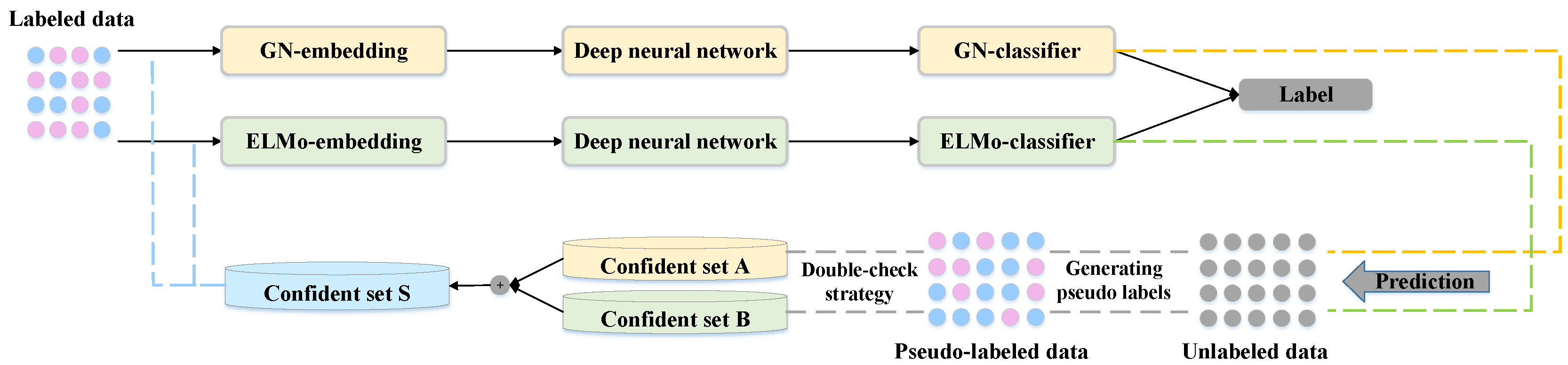
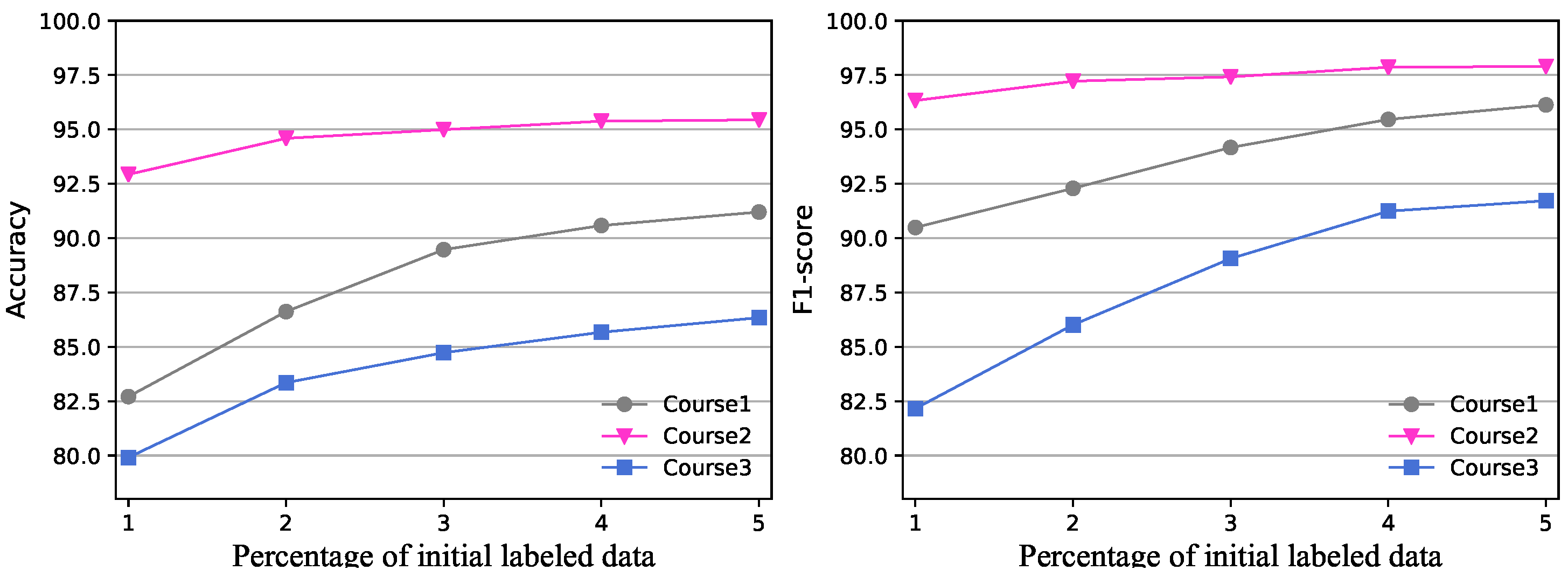
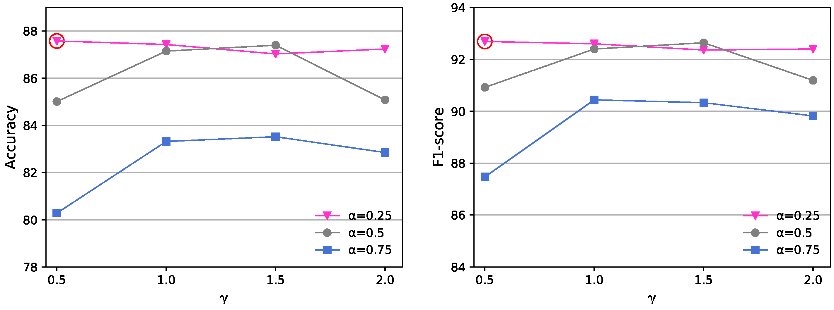
Table 1.
Examples of MOOC forum posts and the corresponding sentiment scores.
| Post | Score |
|---|---|
| I can’t think of a better way to end my holidays than to take this course. I feel my synapses sparkle and feel so inspired. I can’t wait to meet my classes again. | 7 |
| I agree. This will not be automatic for kids until they’ve been shown how. | 4 |
| Terrible interface design! Just put an obvious ’next’ button at the bottom of the main body area or clone the whole linear navigation from the top. | 1 |
Table 2.
The numbers of forum posts for the three courses from the Stanford MOOC Posts dataset.
| Course | Size | Positive | Negative |
|---|---|---|---|
| Education How to Learn Math (Course1) | 9878 | 8188 | 1690 |
| Humanities Science Stat Learning (Course2) | 3030 | 2834 | 196 |
| Medicine Sci Write (Course3) | 5184 | 3907 | 1277 |
Table 3.
Overall performance (%). There are three groups of experiments including the traditional supervised method, deep supervised method, and semi-supervised deep method. SSDL with 30% labeled data for initial training performs much better than all other compared methods.
Table 3.
Overall performance (%). There are three groups of experiments including the traditional supervised method, deep supervised method, and semi-supervised deep method. SSDL with 30% labeled data for initial training performs much better than all other compared methods.
| Method | Course1 | Course2 | Course3 | |||
|---|---|---|---|---|---|---|
| Traditional supervision | Accuracy | F1-score | Accuracy | F1-score | Accuracy | F1-score |
| Random Forest | 83.89 | 89.04 | 92.99 | 94.62 | 79.1 | 81.87 |
| SVM (RBF) | 84.92 | 90.57 | 93.12 | 95.27 | 81.23 | 82.35 |
| Deep supervision | Accuracy | F1-score | Accuracy | F1-score | Accuracy | F1-score |
| GN-CNN | 85.99 | 91.8 | 93.5 | 96.61 | 82.12 | 84.43 |
| ELMo-CNN | 87.29 | 92.41 | 94.16 | 96.95 | 83.46 | 85.57 |
| Deep supervision with FL | Accuracy | F1-score | Accuracy | F1-score | Accuracy | F1-score |
| GN-CNN-FL | 86.36 | 91.97 | 93.83 | 96.79 | 83.57 | 85.41 |
| ELMo-CNN-FL | 87.58 | 92.69 | 94.05 | 96.9 | 84.3 | 86.52 |
| Ours | Accuracy | F1-score | Accuracy | F1-score | Accuracy | F1-score |
| SSDL | 89.47 | 94.17 | 94.99 | 97.42 | 84.73 | 89.06 |
Table 4.
Details of the double-check strategy sample selection of each iteration. There were total six iterations. The same number is the number of samples with same labels predicted by the two classifiers. The augment number is the number of samples added for the training of next iteration. is the similarity threshold to determine the augment number.
| Iteration | Train Number | Test Number | Same Number | Augment Number | |
|---|---|---|---|---|---|
| 1 | 987 | 8891 | 5756 | 576 | 0.4509 |
| 2 | 1563 | 8315 | 7317 | 1463 | 0.397 |
| 3 | 3028 | 6852 | 6372 | 1911 | 0.3624 |
| 4 | 4939 | 4941 | 4348 | 1739 | 0.3454 |
| 5 | 6678 | 3202 | 2689 | 1345 | 0.3318 |
| 6 | 8023 | 1857 | 1819 | 1091 | 0.2992 |
© 2019 by the authors. Licensee MDPI, Basel, Switzerland. This article is an open access article distributed under the terms and conditions of the Creative Commons Attribution (CC BY) license (http://creativecommons.org/licenses/by/4.0/).
Share and Cite
MDPI and ACS Style
Chen, J.; Feng, J.; Sun, X.; Liu, Y. Co-Training Semi-Supervised Deep Learning for Sentiment Classification of MOOC Forum Posts. Symmetry 2020, 12, 8. https://doi.org/10.3390/sym12010008
AMA Style
Chen J, Feng J, Sun X, Liu Y. Co-Training Semi-Supervised Deep Learning for Sentiment Classification of MOOC Forum Posts. Symmetry. 2020; 12(1):8. https://doi.org/10.3390/sym12010008
Chicago/Turabian StyleChen, Jing, Jun Feng, Xia Sun, and Yang Liu. 2020. "Co-Training Semi-Supervised Deep Learning for Sentiment Classification of MOOC Forum Posts" Symmetry 12, no. 1: 8. https://doi.org/10.3390/sym12010008
Note that from the first issue of 2016, this journal uses article numbers instead of page numbers. See further details here.