Modeling of Extreme Values via Exponential Normalization Compared with Linear and Power Normalization

Abstract

Several new asymmetric distributions have arisen naturally in the modeling extreme values are uncovered and elucidated. The present paper deals with the extreme value theorem (EVT) under exponential normalization. An estimate of the shape parameter of the asymmetric generalized value distributions that related to this new extension of the EVT is obtained. Moreover, we develop the mathematical modeling of the extreme values by using this new extension of the EVT. We analyze the extreme values by modeling the occurrence of the exceedances over high thresholds. The natural distributions of such exceedances, new four generalized Pareto families of asymmetric distributions under exponential normalization (GPDEs), are described and their properties revealed. There is an evident symmetry between the new obtained GPDEs and those generalized Pareto distributions arisen from EVT under linear and power normalization. Estimates for the extreme value index of the four GPDEs are obtained. In addition, simulation studies are conducted in order to illustrate and validate the theoretical results. Finally, a comparison study between the different extreme models is done throughout real data sets.

1. Introduction

It has become necessary to study statistical models that have the ability to evaluate these rare phenomena to avoid its dangers due to the sudden rise of some natural harmful phenomena, such as earthquakes, Tsunami, air pollution, and other phenomena. In the last two decades, the EVT has emerged as one of the most significant statistical modeling disciplines for the applied sciences. The EVT can be applied to environmental studies, such as hydrology, pollution, rainfall, floods, wind gusts, and corrosion, in order to develop models for describing the distribution of extreme events. The distributional properties of the extreme and intermediate order statistics and exceedances over (below) high (low) thresholds are determined by the upper and lower tails of the underlying distribution. The most important challenges in any application of such extreme value models is the scarcity of extreme data, choosing the threshold, or beginning of the tail, and choosing the methods of estimating the unknown parameters. Much of the classical EVT is concerned substantially with distribution properties of the maximum $X_{n:n}=max\{X_1,X_2,\dots ,X_n\}$ of iid RVs $X_1,X_2,\dots .,X_n$ and all of the results obtained for maximum of course lead to anologous results for minimum through the obvious relation $X_{1:n}=min\{X_1,X_2,\dots ,X_n\}=-max\{-X_1,-X_2,\dots ,-X_n\}.$ The core of the EVT is the extreme value distributions, which are well known in the literature (cf. [1]), and they are used as approximations to DFs of normalized partial maximum $X_{n:n}$ of iid RVs. A DF F is said to belong to the l-max domain of attraction of an extreme value distribution G under linear normalization, denoted by $F\in D_l\left(G\right),$ if there exist norming constants $a_n>0$ and $b_n\in \mathbb{R}$ such that

$$P\left(\frac{X_{n:n}-b_n}{a_n}\le x\right)=F^n(a_{n}x+b_n)\underset{n}{\overset{w}{⟶}}G\left(x\right),$$

(1)

where “$\underset{n}{\overset{w}{⟶}}$” stands for weak convergence, as $n\to \infty .$ It is well known that the asymptotic relation (1) yields only three possible types of non-degenerate limiting DFs, which are Frèchet, Weibull, and Gumbel DFs. Moreover, any non-degenerate DF G is an extreme value distrbution (i.e., it is a limit in (1)) if and only if it satisfies the stability relation $G^n(a_{n}x+b_n)=G\left(x\right),x\in R,n\ge 1,$ for every integer n, where $a_n>0$ and $b_n\in \mathbb{R}$ are some suitable constants (cf. [1,2]). For this reason, these limits are called l-max-stable laws. On the other hand, these l-max stable laws may be written in the von Mises−Jenkinson format

$$G(x;\mu ,\sigma ,\gamma )=exp[-{[1+\gamma (\frac{x-\mu }{\sigma })]}^{-\frac{1}{\gamma }}],1+\gamma (\frac{x-\mu }{\sigma })>0,$$

(2)

where $\mu$ and $\sigma >0$ are the location and scale parameters, respectively, while $\gamma \in \mathbb{R}$ is a shape parameter that is known as the extreme value index (EVI), which is the central issue in empirical research dealing with extreme events. It is obviously found that the DF $G(x;\mu ,\sigma ,\gamma ),$ which is known as the generalized extreme value distribution under linear normalization (GEVL), describes the Gumbel, Frèchet, and Weibull types with respect to the cases $\gamma =0$ (interpreted as $\gamma \to 0$), $\gamma >0$ and $\gamma <0.$ The GEVL provides a prevailing parametric approache for modeling extreme events, which is known as the block maxima (BM). Its application consists of partitioning a data set into blocks of equal length, and fitting the GEVL to the set of block maxima. An extension of the BM approach is the peak over threshold (POT) approach (see [1]), where we only consider the observations which lie above an appropriate threshold. The generalized Pareto distribution under linear normalization (GPDL) introduced by [3,4] is considered as a foremost pillar of the POT approach. The GPDL is the limit distribution of scaled excesses over high thresholds, which has the form $1+logG(x;\mu ,\sigma ,\gamma ).$

In order to widen the class of limit laws in EVT for solving more approximation problems, the authors of [5] extended the EVT under power normalization ${\left|\frac{X_{n:n}}{{\alpha }_n}\right|}^{\frac{1}{{\beta }_n}}\mathcal{S}\left(X_{n:n}\right),$ where $\mathcal{S}\left(x\right)=sign\left(x\right)=-1,0,1$ according to $x<0,x=0,x>0,$ respectively. Another reason for using the power normalization in EVT is concerning the possibility of getting a better rate of convergence in EVT (cf. [6]). Clearly, the power normalization is a strictly monotone continuous transformation. Therefore, this transformation does not give rise to any wastage of information that the data contains (e.g., the sufficiency property is preserved under one to one transformation). Nevertheless, we might lose some flexibility if we used such normalization. For example, under this normalization we can not change the sign of the data or get rid of zero. The DF F is said to belong to the p-max domain of attraction of a non-degenerate DF H under power normalization, denoted by $F\in D_p\left(H\right)$, if for some norming constants ${\alpha }_n>0$ and ${\beta }_n>0,$

$$P\left({\left|\frac{X_{n:n}}{{\alpha }_n}\right|}^{\frac{1}{{\beta }_n}}\mathcal{S}\left(M_n\right)\le x\right)=F^n\left({\alpha }_n{\left|x\right|}^{{\beta }_n}\mathcal{S}\left(x\right)\right)\underset{n}{\overset{w}{⟶}}H\left(x\right).$$

(3)

The possible p-types of limiting DFs H in (3) are the p-max stable laws satisfying the stability relation $H^n({\alpha }_n{\left|x\right|}^{{\beta }_n}\mathcal{S}\left(x\right))=H\left(x\right),$$x\in \mathbb{R},$ for every $n\ge 1,$ where ${\alpha }_n>0$ and ${\beta }_n>0$ are some suitable sequences of constants. Here, two DFs, F and G, are of the same p-type if we can find $\alpha >0$ and $\beta >0,$ for which $F\left(x\right)=G(\alpha {\left|x\right|}^{\beta }\mathcal{S}\left(x\right)),$ for all $x.$ Consequently, any non-degenerate DF H is a p-max stable, or equivalently H is a limit in (3), if and only if for every $n\ge 1$ the two DFs H and $H^n$ are of the same p-type. In [7] the author has exemplified these types by the von Mises representation $P_{i;\gamma }(x;a,b)=exp\left[-{(-1)}^i{(1-\gamma loga{(-{(-1)}^{i}x)}^b)}^{-\frac{1}{\gamma }}\right],{(-1)}^{i}x<0,1-{(-1)}^i\gamma loga{(-{(-1)}^{i}x)}^b>0,i=1,2.$ Each of these families is called generalized extreme value distribution under power normalization (GEVP). It is well known that the p-max-stable laws attract more distributions than the l-max-stable laws. This fact virtually means that the linear model may be unsuccessful for fitting an extreme data set; on the contrary, the power model succeed to fit it (see [1]). The authors of [8] applied the BM approach under power normalization using the GEVPs. Moreover, in a series of papers, refs. [9,10,11,12,13] developed the modeling of extreme values under power normalization by defining and using the generalized Pareto distributions under power normalization (GPDPs), $1+log{P}_{i;\gamma }(x;1,1),i=1,2,$ to a real extreme-value data (for more details regarding the power transformation, see [14,15,16,17,18]).

Once more, in order to widen the class of the limit laws in EVT, in [19] the authors extended the EVT under exponential normalization ${\mathcal{T}}_n\left(x\right)={\mathcal{T}}_{u_n,v_n}\left(x\right)=exp\{u_n{\left(\right|log\left|x\right|\left|\right)}^{v_n}$$\mathcal{S}(log|x\left|\right)\left\}\mathcal{S}\right(x),$$u_n,v_n>0.$ Under this transformation, we can say that the DFs F and G are of the same e-type if $F\left(x\right)={G(exp\{\left(u\right(|log|x\left|\right|)}^v\mathcal{S}(log|x\left|\right)\left)\right\}\mathcal{S}\left(x\right))=G\left({\mathcal{T}}_{u,v}\left(x\right)\right),$ for some constants $u>0,$$v>0.$ In this case, a non-degenerate DF $\mathsf{\Lambda }(·)$ is said to be an e-max-stable laws if there exists a DF F and norming constants $u_n>0,v_n>0$, such that

$$\begin{array}{ccc}\hfill P\left({\mathcal{T}}_n^{-}\left(X_{n:n}\right)\right\}\le x)& =& P\left(\left\{\left[exp({\left(\frac{|log|X_{n;n}\left|\right|}{u_n}\right)}^{1/v_n}\mathcal{S}(log|X_{n:n}\left|\right))\right]\right\}\mathcal{S}\left(X_{n:n}\right)\le x\right)\hfill \\ \hfill & =& P(X_{n:n}\le {\mathcal{T}}_n\left(x\right))=F^n\left({\mathcal{T}}_n\left(x\right)\right)\underset{n}{\overset{w}{⟶}}\mathsf{\Lambda }\left(x\right).\hfill \end{array}$$

(4)

If (4) is satisfied, then we can say that the DF F belongs to the e-max-domain of attraction of the non-degenerate DF $\mathsf{\Lambda }$ under e-normalization, denoted by $F\in D_e\left(\mathsf{\Lambda }\right).$ The authors of [19], showed that the possible limiting DFs $\mathsf{\Lambda }$ in (4) are the e-max stable laws that satisfy the stability property that any non-degenerate DF $\mathsf{\Lambda }$ is an e-max stable, or equivalently $\mathsf{\Lambda }$ is a limit in (4), if and only if for every $n\ge 1$ the two DFs $\mathsf{\Lambda }$ and ${\mathsf{\Lambda }}^n$ are of the same e-type (for more details about the exponential transformation, see [20]).

In [19], the authors showed that the possible limit laws arisen from (4) attract more DFs than the p-max-stable laws. This fact virtually means that the linear and power models may fail to fit the given extreme data, while the exponential model succeeds. This fact gives us a sufficient motivation for developing the modeling of extreme values via the exponential model, denoted by the e-model. The aimed development is the first object of this paper and it will be achieved within two stages. the first stage is to infer the generalized extreme value distributions related to the EVT under exponential normalization. These asymmetric DFs enable us to apply the BM approach. The second stage is deriving the possible generalized Pareto families of asymmetric distributions relating to the EVT under exponential normalization. These families will pave the way to applying the POT approach. The second object of this paper is comparing between the EVT under linear, power, and exponential normalization via a real data sets of air pollution.

The rest of this paper is structured, as follows: In Section 2, we deduce the generalized extreme value distributions relating to the EVT under exponential normalization (GEGEs). In Section 3, which is devoted to the theoretical details, we first suggest an estimate for the EVI in each of the GEGEs. This estimate corresponds to a Dubey estimate in the GEVL model (3) and the GEVP models $P_{i\gamma }(x;a,b),i=1,2$ (cf. [8]). Secondly, we derive the generalized Pareto distributions under exponential normalization (GPDEs). Finally, we propose estimators for the EVI in these GPDEs. Section 4 is devoted to a simulation study, which illustrates and corroborates the theoretical results. In Section 5, the EVT under linear, power, and exponential normalization is applied, with comparisons to several real data sets.

2. Preliminary Results

In [19], the authors derived the following a chain of equivalences between l-max-domains, p-max-domains and e-max-domains of attraction:

• $F_X\in D_l\left(F_{\xi }\right)⟺F_{exp\left(X\right)}\in D_p\left(F_{exp\left(\xi \right)}\right)⟺F_{-exp(-X)}\in D_p\left(F_{-exp(-\xi )}\right),$ where $F_{\xi }$ is an l-max stable DF, and $F_{exp\left(\xi \right)}$ and $F_{-exp(-\xi )}$ are p-max stable DFs.
• $F_X\in D_p\left(F_{\xi }\right)⟺F_{exp\left(X\right)}\in D_e\left(F_{exp\left(\xi \right)}\right)⟺F_{-exp(-X)}\in D_e\left(F_{-exp(-\xi )}\right),$ where $F_{\xi }$ is an p-max stable DF, and $F_{exp\left(\xi \right)}$ and $F_{-exp(-\xi )}$ are e-max stable laws.

In the above implications, $F_X$ denotes the DF of the RV X and “$⟺$” stands for “if and only if”. Moreover, ref. [19] used these implications in order to determine e-max-stable laws, wherein the first six e-max-stable DFs have right endpoint $r\left(\mathsf{\Lambda }\right)=sup\{x:\mathsf{\Lambda }(x)<1\}>0$ and the subsequent six e-max-stable DFs have $r\left(\mathsf{\Lambda }\right)\le 0.$

$$\left.\begin{array}{cc}1:{\mathsf{\Lambda }}_{1,\beta }\left(x\right)=exp(-{(loglogx)}^{-\beta }),x\ge e;\hfill & \\ 2:{\mathsf{\Lambda }}_{2,\beta }\left(x\right)=exp(-{(-loglogx)}^{\beta }),1\le x<e;\hfill & \\ 3:{\mathsf{\Lambda }}_{3,\beta }\left(x\right)=exp(-{(logx)}^{-1}),x\ge 1;\hfill & \\ 4:{\mathsf{\Lambda }}_{4,\beta }\left(x\right)=exp(-{(-log(-logx))}^{-\beta }),1/e\le x<1;\hfill & \\ 5:{\mathsf{\Lambda }}_{5,\beta }\left(x\right)=exp(-{(log(-logx))}^{\beta }),0\le x<1/e;\hfill & \\ 6:{\mathsf{\Lambda }}_{6,\beta }\left(x\right)=x,0\le x<1;\hfill & \\ 7:{\mathsf{\Lambda }}_{7,\beta }\left(x\right)=exp(-{(log(-log(-x)))}^{-\beta }),-1/e\le x<0;\hfill & \\ 8:{\mathsf{\Lambda }}_{8,\beta }\left(x\right)=exp(-{(-log(-log(-x)))}^{\beta }),-1\le x<-1/e;\hfill & \\ 9:{\mathsf{\Lambda }}_{9,\beta }\left(x\right)=exp(-{(-log(-x))}^{-1}),-1\le x<0;\hfill & \\ 10:{\mathsf{\Lambda }}_{10,\beta }\left(x\right)=exp(-{(-loglog(-x))}^{-\beta }),-e\le x<-1;\hfill & \\ 11:{\mathsf{\Lambda }}_{11,\beta }\left(x\right)=exp(-{(loglog(-x))}^{\beta }),x\le -e;\hfill & \\ 12:{\mathsf{\Lambda }}_{12,\beta }\left(x\right)={\mathsf{\Lambda }}_{12}\left(x\right)=-\frac{1}{x},x\le -1.\hfill \end{array}\right\}$$

(5)

We now totalize the limit laws (5) using the von Mises type representations. For any $a,b>0,$ the types (5) are totalized by the following general von Mises type forms:

$$\left.\begin{array}{cc}{W}_{1;\gamma }(x;a,b)=exp[-{(1+\gamma log\left(a{(logx)}^b\right))}^{\frac{-1}{\gamma }}],1+\gamma log\left(a{(logx)}^b\right)>0;& \\ W_{2;\gamma }(x;a,b)=exp[-{(1+\gamma (-log\left(a{(-logx)}^b\right)))}^{\frac{-1}{\gamma }}],1+\gamma (-log\left(a{(-logx)}^b\right))>0;& \\ W_{3;\gamma }(x;a,b)=exp[-{(1+\gamma log\left(a{(-log(-x))}^b\right))}^{\frac{-1}{\gamma }}],1+\gamma log\left(a(-log(-x))\right)>0;& \\ W_{4;\gamma }(x;a,b)=exp[-{(1+\gamma (-log\left(a{(log(-x))}^b\right)))}^{\frac{-1}{\gamma }}],1+\gamma (-log\left(a{(log(-x))}^b\right)>0,\end{array}\right\}$$

(6)

where $\gamma$ is a given real number. When $\gamma =0,W_{i;\gamma }(x;a,b)$ is defined as ${lim}_{\gamma \to 0}{W}_{i;\gamma }(x;a,b),$$i=1,2,3,4.$ The DF $W_{i;\gamma }(x;a,b)$ yields laws of the same e-types as ${\mathsf{\Lambda }}_{3i-2}\left(x\right),{\mathsf{\Lambda }}_{3i-1}\left(x\right)$ and ${\mathsf{\Lambda }}_{3i}\left(x\right),i=1,2,3,4,$ according to $\gamma =\frac{1}{\beta }>0,\gamma =-\frac{1}{\beta }<0$ and $\gamma =0(\gamma \to 0),$ respectively. Each DF in (6) is called generalized extreme value distribution under exponential normalization (GEVE), denoted by GEVE$(\gamma ,a,b).$ Clearly, the parametric models in (6) enable us to apply the BM approach under exponential normalization, where, in this case, we have to assume that the data in hand form a random sample drwan from an exact GEVE$(\gamma ,a,b).$

3. BM Approach and GPDEs

When considering the BM approach, let $x_{1:n}\le x_{2:n}\le \cdots \le x_{n:n}$ be the set of maximums of the given blocks. Clearly, in view of the shape of the e-types (6), the modeling under exponential normalization can only be applied if all values of these maximums belong to one and only one of the non-overlapping intervals ${\mathcal{I}}_1=(1,\infty ),{\mathcal{I}}_2=(0,1),{\mathcal{I}}_3=(-1,0)$ and ${\mathcal{I}}_4=(-\infty ,-1).$ More specifically, if $1<x_{1:n}\le x_{2:n}\le \cdots \le x_{n:n},$ or $0<x_{1:n}\le x_{2:n}\le \cdots \le x_{n:n}<1,$ or $-1<x_{1:n}\le x_{2:n}\le \cdots \le x_{n:n}<0,$ or $x_{1:n}\le x_{2:n}\le \cdots \le x_{n:n}<-1,$ we would select the model $W_{1;\gamma }(x;a,b),$ or $W_{2;\gamma }(x;a,b),$ or $W_{3;\gamma }(x;a,b),$ or $W_{4;\gamma }(x;a,b),$ respectively. Subsequently, we compute the maximum likelihood (ML) estimates $(\widehat{\gamma },\widehat{a},\widehat{b})$ of $(\gamma ,a,b)$ as the numerical solutions of the likelihood equations based on the selected model. The estimate of the shape parameter $\gamma$ corresponds to a Dubey estimate in the GEVL model is linear combinations of ratios of spacing

$$R_n=\left\{\begin{array}{c}\frac{log(log\left(X_{n{q}_2:n}\right))-log(log\left(X_{n{q}_1:n}\right))}{log(log\left(X_{n{q}_1:n}\right))-log(log\left(X_{n{q}_0:n}\right))},\mathrm{for\; the\; model}{\mathrm{W}}_{1;\gamma },\hfill \\ \frac{log(-log\left(X_{n{q}_2:n}\right))-log(-log\left(X_{n{q}_1:n}\right))}{log(-log\left(X_{n{q}_1:n}\right))-log(-log\left(X_{n{q}_0:n}\right))},\mathrm{for\; the\; model}{\mathrm{W}}_{2;\gamma },\hfill \\ \frac{log(-log(-X_{n{q}_2:n}))-log(-log(-X_{n{q}_1:n}))}{log(-log(-X_{n{q}_1:n}))-log(-log(-X_{n{q}_0:n}))},\mathrm{for\; the\; model}{\mathrm{W}}_{3;\gamma },\hfill \\ \frac{log(log(-X_{n{q}_2:n}))-log(log(-X_{n{q}_1:n}))}{log(log(-X_{n{q}_1:n}))-log(log(-X_{n{q}_0:n}))},\mathrm{for\; the\; model}{\mathrm{W}}_{4;\gamma },\hfill \end{array}\right.$$

where $q_0<q_1<q_2$ and $q_i=\frac{i}{n}.$ Clearly, the statistic $R_n$ is invariant under the exponential transformation. Now, relaying on the obvious relations: (1) $F_{t;n}^{-1}\left(q_i\right)=x_{i:n},$ where $t=1,$ or $t=2,$ or $t=3,$ or $t=4,$ if $x_{i:n}\in {\mathcal{I}}_1,i=1,2,\dots ,n,$ or $x_{i:n}\in {\mathcal{I}}_2,i=1,2,\dots ,n,$ or $x_{i:n}\in {\mathcal{I}}_3,i=1,2,\dots ,n,$ or $x_{i:n}\in {\mathcal{I}}_4,i=1,2\dots ,n,$ respectively, and $F_{t;n}$ is the sample DF, (2) for large $n,$ we have $F_{t;n}\left(x\right)\simeq F^n\left(x\right)\simeq W_{t;\gamma }\left({\mathcal{T}}_n^{-}\left(x\right)\right)$ and (3) $F_{t;n}^{-1}\left({\mathcal{T}}_n\left(x\right)\right)={\mathcal{T}}_n^{-}\left(F_{t;n}^{-1}\left(x\right)\right),$ we obtain

$$R_n=\frac{log\left(\right|log|W_{t;\gamma }^{-1}\left(q_2\right|)\left|\right)-log\left(\right|log|W_{t;\gamma }^{-1}\left(q_1\right)\left|\right)|}{log\left(\right|log|W_{t;\gamma }^{-1}\left(q_1\right|)\left|\right)-log\left(\right|log|W_{t;\gamma }^{-1}\left(q_0\right|)\left|\right)},t=1,\dots ,4.$$

(7)

The relation (7), after some algebra, yields

$$R_n=\frac{{(-log{q}_2)}^{-\gamma }-{(-log{q}_1)}^{-\gamma }}{{(-log{q}_1)}^{-\gamma }-{(-log{q}_0)}^{-\gamma }}={\left(\frac{log{q}_0}{log{q}_2}\right)}^{\frac{\gamma }{2}},$$

(8)

if $q_0,q_1,q_2$ satisfy the equation ${(-log{q}_1)}^2=(-log{q}_2)(-log{q}_0).$ Upon taking the logarithm of both sides of (8), we get the estimate

$$\widehat{\gamma }=\frac{2log{R}_n}{log(log{q}_0/log{q}_2)}.$$

On the other hand, if $q_0=q,q_1=q^a,q_2=q^{a^2},$ for some $0<q,a<1,$ we get the estimate family $\widehat{\gamma }=\frac{log{R}_n}{-loga}.$ By taking $a=\frac{1}{2},$ we get

$${\widehat{\gamma }}_e=\frac{log{R}_n}{log2}.$$

(9)

In Section 4, we will compare the ML method and estimate ${\widehat{\gamma }}_e$ for estimating $\gamma$ via the $W_{1;\gamma }^{-1}.$ Moreover, we will detect the value of $q,$ which gives the best estimate for $\gamma .$ It will be revealed that the estimate (9) is very poor for large values of $\gamma$ ($\gamma >0.1).$ Regardless of the fact that this estimate is based on the BM approach, this approach also suffers some other problems, among them is only considering several maxima within several blocks and ignoring most the other data. In a spirit of the result of [3,4], we propose applying the POT approach based on the EVT under exponential normalization, where we deal with the right tail $\overline{F}\left(x\right)=1-F\left(x\right),$ for large $x,$ i.e., we deal with top-order observations. In order to adapt this approach for the e-model we derive the GPDE. Our focus will be mainly on the case $r\left(F\right)>0$ via Theorem 1. Clearly, the case $r\left(F\right)>0$ covers most of the important practical applications of the EVT. However, the case $r\left(F\right)<0$ will be briefly discussed in Theorem 3. In the next theorems and throughout the paper, we adopt the notations $F^{\left[A\right]}\left(x\right)=P(X\le x)\mid X>A)$ and “$\underset{n}{⟶}$” to mean convergence as $n\to \infty .$

Theorem 1.

Let (4) be satisfied with$W_{t;\gamma }(x;a,b),t\in \{1,2\}.$Then there exists$\alpha \left(u\right)>0$such that

$$F^{\left[e^{{(-1)}^{t+1}u}\right]}\left({\mathcal{T}}_{u,\alpha \left(u\right)}\left(x\right)\right)\underset{u}{\overset{w}{⟶}}{Q}_t\left(x\right),$$

(10)

where “$\underset{u}{\overset{w}{⟶}}$” means weak convergence, as$e^{{(-1)}^{t+1}u}\uparrow r\left(F\right)$and

a.

$Q_1\left(x\right)=Q_{1;\gamma }(x;\overline{b})=1+log{W}_{1;\gamma }(x;1,\overline{b}),$$\overline{b}=\frac{b}{c}$and$c=1+\gamma loga,$if$r\left(F\right)>1$;

b.

$Q_2\left(x\right)=Q_{2;\gamma }(x;\underline{b})=1+log{W}_{2;\gamma }(x;1,\underline{b}),$$\underline{b}=\frac{b}{\underline{c}}$and$\underline{c}=1-\gamma loga,$if$0<r\left(F\right)\le 1.$

Proof. 

The proof of Part [a]: In view of the EVT, we obtain

$$n(1-F\left({\mathcal{T}}_{u_n,v_n}\left(x\right)\right))\underset{n}{\overset{}{⟶}}-log{W}_{1;\gamma }(x;a,b),$$

which, in view of the assumption $r\left(F\right)>1,$ implies that

$$n(1-F(exp(u_n{(logx)}^{v_n})))\underset{n}{\overset{}{⟶}}-log{W}_{1;\gamma }(x;a,b).$$

(11)

On the other hand, (11) cannot be true unless $F(exp(u_n{(logx)}^{v_n}))\underset{n}{\overset{}{⟶}}1,$ for all x for which $W_{1;\gamma }(x;a,b)>0.$ Thus, we can write

$$\begin{array}{ccc}\hfill n(1-F(exp(u_{n+1}{(logx)}^{v_{n+1}})))& \simeq & (n+1)(1-F(exp(u_{n+1}{(logx)}^{v_{n+1}})))\hfill \end{array}$$

$$\underset{n}{\overset{}{⟶}}-log{W}_{1;\gamma }(x;a,b).$$

(12)

By using the modified Khinchin’s Theorem (cf. [1]), the relations (11) and (12) yield

$${\left(\frac{u_{n+1}}{u_n}\right)}^{\frac{1}{v_n}}\underset{n}{\overset{}{⟶}}1and\frac{v_{n+1}}{v_n}\underset{n}{\overset{}{⟶}}1.$$

(13)

Now, let n be chosen, such that $u_n\le u\le u_{n+1},$ where u is any real number such that $e^u<r\left(F\right)$ (note that by putting $x=e$ in (11), we get $e^{u_n}\uparrow r\left(F\right)$). Subsequently, (13) implies that $1={\left(\frac{u}{u_n}\right)}^{\frac{1}{v_n}}\le {\left(\frac{u_{n+1}}{u_n}\right)}^{\frac{1}{v_n}}\to 1.$ Thus, put $\alpha \left(u\right)\equiv v_n$ and apply again the modified Khinchin’s Theorem, (11) may be written in the form

$$n(1-F(exp(u{(logx)}^{\alpha \left(u\right)})))\underset{n}{\overset{}{⟶}}-log{W}_{1;\gamma }(x;a,b).$$

(14)

Therefore, by putting $x=e$ in (14), we get

$$n(1-F(exp(u)))\to {\left[1+\gamma loga\right]}^{-\frac{1}{\gamma }}.$$

(15)

By combining (14) and (15), we get, as $n\to \infty ,$ or equivalently as $e^u\uparrow r\left(F\right)$,

$$\begin{array}{ccc}\hfill F^{\left[e^u\right]}\left({\mathcal{T}}_{u,\alpha \left(u\right)}\left(x\right)\right)& =& \frac{F\left({\mathcal{T}}_{u,\alpha \left(u\right)}\left(x\right)\right)-F(exp(u))}{1-F(exp(u))}=1-\frac{1-F\left({\mathcal{T}}_{u,\alpha \left(u\right)}\left(x\right)\right)}{1-F(exp(u))}\hfill \\ & \underset{u}{\overset{w}{⟶}}& 1-\frac{W_{1;\gamma }(x;a,b)}{W_{1;\gamma }(e;a,b)}=1-{\left(\frac{1+\gamma log\left(a{(logx)}^b\right)}{1+\gamma loga}\right)}^{-\frac{1}{\gamma }}\hfill \\ & =& 1-{\left[1+\overline{b}\gamma z\right]}^{-\frac{1}{\gamma }}=1+log{W}_{1;\gamma }(x;1,\overline{b}),\hfill \end{array}$$

which was to be proved. The proof of Part [b] is very similar to the proof of Part [a], with the exception of only of obvious changes. This completes the proof of Theorem 1. □

Theorem 2

(the peak over threshold stability property). The left truncated GPDE again yields a GPDE. This means that, for every $1<L<x,$ we have $Q_{1;\gamma }^{\left[L\right]}(x;\sigma )=Q_{1;\gamma }(\frac{x}{L};\overline{\sigma }),$ where $\overline{\sigma }=\frac{\sigma }{c}$ and $c=1+\gamma \sigma logL.$ Moreover, for every $0<L<x<1,$ we have $Q_{2;\gamma }^{\left[L\right]}(x;\sigma )=Q_{2;\gamma }(\frac{x}{L};\overline{\sigma }),$ where $\overline{\sigma }=\frac{\sigma }{\overline{c}}$ and $\overline{c}=1-\gamma \sigma log(-L).$

Proof. 

Let $L\le x.$ Subsequently,

$$\begin{array}{ccc}\hfill Q_{1;\gamma }^{\left[L\right]}(x;\sigma )& =& \frac{1-{(1+\gamma \sigma log(logx))}^{-\frac{1}{\gamma }}-(1-{(1+\gamma \sigma logL)}^{-\frac{1}{\gamma }})}{1-(1-{(1+\gamma \sigma logL)}^{-\frac{1}{\gamma }})}\hfill \\ & =& \frac{{(1+\gamma \sigma logL)}^{-\frac{1}{\gamma }}-{(1+\gamma \sigma log(logx))}^{-\frac{1}{\gamma }}}{{(1+\gamma \sigma logL)}^{-\frac{1}{\gamma }}}=1-\frac{{(1+\gamma \sigma log(logx))}^{-\frac{1}{\gamma }}}{{(1+\gamma \sigma logL)}^{-\frac{1}{\gamma }}}\hfill \\ & =& 1-{\left[\frac{(1+\gamma \sigma log(logx\left)\right)}{(1+\gamma \sigma logL)}\right]}^{-\frac{1}{\gamma }}=1-{(1+\frac{\gamma \sigma log\left(\frac{logx}{L}\right)}{c})}^{-\frac{1}{\gamma }},\hfill \end{array}$$

where $c=1+\gamma \sigma logL.$ On the other hand, we have

$$\begin{array}{ccc}\hfill Q_{2;\gamma }^{\left[L\right]}(x;\sigma )& =& \frac{{(1-\gamma \sigma log(-L))}^{-\frac{1}{\gamma }}-{(1-\gamma \sigma log(-logx))}^{-\frac{1}{\gamma }}}{{(1-\gamma \sigma log(-L))}^{-\frac{1}{\gamma }}}\hfill \\ & =& 1-\frac{{(1-\gamma \sigma log(-logx))}^{-\frac{1}{\gamma }}}{{(1-\gamma \sigma log(-L))}^{-\frac{1}{\gamma }}}=1-{(1-\frac{\gamma \sigma log(-\left(\frac{-logx}{L}\right))}{c})}^{-\frac{1}{\gamma }},\hfill \end{array}$$

where $c=1-\gamma \sigma log(-L).$ This completes the proof of Theorem 2. □

Theorem 3.

Let (4) be satisfied with$W_{t;\gamma }(x;a,b),t\in \{3,4\}.$Subsequently, there exists$\alpha \left(u\right)>0$such that$F^{[-e^{{(-1)}^{t}u}]}\left({\mathcal{T}}_{u,\alpha \left(u\right)}\left(x\right)\right)\underset{u}{\overset{w}{⟶}}{Q}_t\left(x\right),$where “$\underset{u}{\overset{w}{⟶}}$” means weak convergence, as$-e^{{(-1)}^{t}u}\uparrow r\left(F\right)$and

c.

$Q_{3;\gamma }(x;\overline{b})=1+log{W}_{3;\gamma }(x;1,\overline{b}),$if$-1<r\left(F\right)<0$;

d.

$Q_{4;\gamma }(x;\underline{b})=1+log{W}_{4;\gamma }(x;1,\underline{b}),$if$r\left(F\right)<-1.$

Moreover, the limits$Q_{3;\gamma }(x;\overline{b})$and$Q_{4;\gamma }(x;\underline{b})$satisfy the peak over threshold stability property.

Proof. 

The proof is very similar to the proof of Theorems 1 and 2, with the exception of only of obvious changes. □

Estimation of the EVI via GPDE Model

In this subsection, we derive estimates for the parametrs $\gamma$ and $\overline{\sigma }$ in the GPDE $Q_{1;\gamma }(x;\sigma ).$ These estimates consort with the Pickand’s estimates in the GEVL model (2) (cf. [4]). Let n be the sample size and $m=m\left(n\right)$ be an integer much smaller than $n.$ Let $X_i^{\star }=X_{n-i+1:n}$ be the ith largest observation in the sample, $i=1,2,\dots ,n.$ The values $\frac{X_i^{\star }}{X_{4m}^{\star }},i=1,2,\dots ,4m-1,$ will be treated as though they were the descending order statistics from a sample of size $4m-1$ from the DF $Q_{1;\gamma }(x;\sigma )$ for some $0<\sigma <\infty$ and $-\infty <\gamma <\infty .$ Because, for any $0\le y\le 1,$ we have $Q_{1,\gamma }^{-1}(y;\sigma )=exp\left[exp\left[\frac{1}{\gamma \sigma }({(1-y)}^{-\gamma }-1)\right]\right],$ we get $Q_{1,\gamma }^{-1}\left(\frac{1}{2};\sigma \right)=exp\left[e^{\frac{1}{\gamma \sigma }\left(2^{\gamma }-1\right)}\right]$ and $Q_{1,\gamma }^{-1}\left(\frac{3}{4};\sigma \right)=exp\left[e^{\frac{1}{\gamma \sigma }\left(2^{2\gamma }-1\right)}\right].$ Clearly,

$$\mathcal{L}=\frac{log(log{Q}_{1,\gamma }^{-1}(\frac{3}{4};\sigma ))-log(log{Q}_{1,\gamma }^{-1}(\frac{1}{2};\sigma ))}{log(log{Q}_{1,\gamma }^{-1}\left(\frac{1}{2}\right);\sigma )}=2^{\gamma },$$

which implies $\gamma =\frac{log\mathcal{L}}{log2}$ and $\sigma =\frac{2^{\gamma }-1}{\gamma log{Q}_{1,\gamma }^{-1}(\frac{1}{2};\sigma )}.$ To estimate $\gamma$ and $\sigma$, we replace the population quantiles $Q_{1,\gamma }^{-1}\left(\frac{1}{2};\sigma \right)$ and $Q_{1,\gamma }^{-1}\left(\frac{3}{4};\sigma \right)$ by the sample quantiles ${\widehat{Q}}_{1,\gamma }^{-1}\left(\frac{1}{2};\sigma \right)=\frac{X_{2m}^{\star }}{X_{4m}^{\star }}$ and ${\widehat{Q}}_{1,\gamma }^{-1}\left(\frac{3}{4};\sigma \right)=\frac{X_m^{\star }}{X_{4m}^{\star }}.$ Therefore,

$$\widehat{\gamma }={\left(log2\right)}^{-1}log\frac{log{X}_m^{\star }-log{X}_{2m}^{\star }}{log{X}_{2m}^{\star }-log{X}_{4m}^{\star }}and\widehat{\sigma }=\frac{2^{\widehat{\gamma }}-1}{\widehat{\gamma }(log{X}_{2m}^{\star }-log{X}_{4m}^{\star })}.$$

(16)

In the next section, we will consider the determination problem of m via a simulation study. Theoretically, the value $m=m\left(n\right)$ should satisfy the two conditions ${lim}_{n\to \infty }m=\infty$ and ${lim}_{n\to \infty }\frac{m}{n}=0$ (cf. [4]).

4. Simulation Study

In

Table 1. Estimating the extreme value index (EVI) $\gamma$ via $W_{1;\gamma }(x;2\times {10}^{-3},10)$ by using the maximum likelihood (ML) and (9) estimators.

$\mathit{\gamma }$		ML Estimate	The Estimate (9)
			$\mathit{q}=\mathbf{0.6}$	$\mathit{q}=\mathbf{0.68}$	$\mathit{q}=\mathbf{0.7}$	$\mathit{q}=\mathbf{0.75}$	$\mathit{q}=\mathbf{0.8}$
0.08	$\widehat{{\gamma }_e}$	0.0800	−0.0267	0.0496	0.0520	0.0411	0.0819
	MSE	$5.22\times {10}^{-4}$	1.1394	0.0926	0.0786	0.1513	$3.54\times {10}^{-4}$
0.09	$\widehat{{\gamma }_e}$	0.0896	−0.0718	0.0062	0.0256	0.0871	0.1349
	MSE	$4.98\times {10}^{-4}$	2.6172	0.7018	0.4141	$8.15\times {10}^{-4}$	0.2015
0.1	$\widehat{{\gamma }_e}$	0.1037	0.0341	0.1062	0.0899	0.1182	0.1700
	MSE	$5.06\times {10}^{-4}$	0.4344	0.0039	0.0101	0.0330	0.4899
0.11	$\widehat{{\gamma }_e}$	0.1095	0.0327	0.1096	0.1094	0.1435	0.1992
	MSE	$6.41\times {10}^{-4}$	0.5977	$1.73\times {10}^{-5}$	$3.44\times {10}^{-5}$	0.1125	0.7959
0.12	$\widehat{{\gamma }_e}$	0.1215	0.0775	0.1517	0.1476	0.1872	0.2714
	MSE	$4.57\times {10}^{-4}$	0.1809	0.1003	0.0762	0.4511	2.2913

, we compare the ML method and the Formula (9) for estimating the EVI $\gamma$ via the first GEVE defined in (6). Additionally, from Table 1, we determine the value of $q,$ which gives the best estimate for $\gamma .$ In Table 1, we present estimates for each value of $\gamma =0.08,0.09,0.1,0.11,0.12$ by applying the ML method and computing the estimate ${\widehat{\gamma }}_e$ that resulted from (9) for different quantiles $q=0.6,0.68,0.7,0.75,0.8.$ This procedure is repeated 1000 times to obtain the average estimates (for the given different values of q) for $\gamma$ and their mean square errors (MSE’s). Table 1 shows that the estimates (9) are poor when compared with the Ml estimates. Moreover, the precision of the estimate ${\widehat{\gamma }}_e$ closely depends on the value of $\gamma .$ It was revealed that when $\gamma >0.12,$ the estimates computed by (9) became very poor, for this reason in Table 1 we only considered the values $\gamma \le 0.12.$

In

Table 2. Estimating the EVI $\gamma$ in the generalized Pareto distributions under exponential normalization (GPDE) $Q_{1;\gamma },$ by using the ML method.

k	5000	4500	4000	3500	3000	2500	2000	1000
The GPDE $Q_{1;\gamma },$ with $\gamma =0.08$
$\widehat{\gamma }$	0.0486	0.0522	0.0618	0.0665	0.0679	0.0738	0.0756	$0.0761{}^{\star }$
MSE	0.0011	0.0009	0.0006	0.0003	0.0003	0.0003	0.0004	0.0004
The GPDE $Q_{1;\gamma },$ with $\gamma =0.09$
$\widehat{\gamma }$	0.0488	0.0475	0.0576	0.0653	0.0724	0.0729	0.0727	$0.0832{}^{\star }$
MSE	0.0018	0.0019	0.0012	0.0008	0.0005	0.0005	0.0006	0.0003
The GPDE $Q_{1;\gamma },$ with $\gamma =0.1$
$\widehat{\gamma }$	0.0700	0.0702	0.0724	0.0720	0.0794	0.0835	$0.0924{}^{\star }$	0.0924
MSE	0.0011	0.0012	0.0010	0.0010	0.0006	0.0005	0.0002	0.0003
The GPDE $Q_{1;\gamma },$ with $\gamma =0.11$
$\widehat{\gamma }$	0.0785	0.0854	0.0884	0.0920	0.0945	0.1006	$0.1021{}^{\star }$	0.1189
MSE	0.0011	0.0008	0.0007	0.0004	0.0004	0.0002	0.0002	0.0004
The GPDE $Q_{1;\gamma },$ with $\gamma =0.12$
$\widehat{\gamma }$	0.0894	0.0949	0.0983	0.1038	0.1113	0.1133	0.1143	$0.1173{}^{\star }$
MSE	0.0011	0.0007	0.0006	0.0004	0.0004	0.0011	0.0007	0.0005

, for each value of $\gamma =0.08,0.09,0.1,0.11,0.12$ we generate a random sample of size $n=20,000$ from $Q_{1;\gamma }(x;1).$ Moreover, we choose the threshold values $k=5000,4500,$$\dots ,1000$ (in the interval $k\le \frac{n}{4}$). In view of Theorem 2, the DF of the simulated data, which come after any threshold value $k,$ has the same type of the DF $Q_{1;\gamma }.$ Therefore, we can estimate the parameter $\gamma$ by using the ML method for each of these threshold values. This procedure is repeated 1000 times to obtain the average estimates and their MSE’s. Finally, we determine the value $k,$ which gives the best estimate for the parameter $\gamma$ by using the ML method.

Table 3. Estimating the EVI $\gamma$ in the GPDE $Q_{1;\gamma },$ by using the estimator (16).

m	125	250	375	500	625	750	1000	1250
The GPDE $Q_{1;\gamma },$ with $\gamma =0.08$
$\widehat{\gamma }$	0.0794	0.0858	0.0883	0.0818	0.0784	0.0819	$0.0801{}^{\star }$	0.0808
MSE	0.0047	0.0026	0.0021	0.0013	0.0012	0.0009	0.0007	0.0006
The GPDE $Q_{1;\gamma },$ with $\gamma =0.09$
$\widehat{\gamma }$	0.0924	0.0865	0.0845	0.0895	0.0911	$0.0905{}^{\star }$	0.0913	0.0917
MSE	0.0048	0.0024	0.0019	0.0016	0.0012	0.0010	0.0008	0.0007
The GPDE $Q_{1;\gamma },$ with $\gamma =0.1$
$\widehat{\gamma }$	0.1041	0.0967	0.0957	0.0992	$0.1002{}^{\star }$	0.0995	0.0987	0.1011
MSE	0.0061	0.0027	0.0018	0.0013	0.0015	0.0010	0.0009	0.0007
The GPDE $Q_{1;\gamma },$ with $\gamma =0.11$
$\widehat{\gamma }$	$0.1099{}^{\star }$	0.1166	0.1132	0.1103	0.1103	0.1137	0.1136	0.1136
MSE	0.0047	0.0028	0.0013	0.0014	0.0009	0.0010	0.0009	0.0008
The GPDE $Q_{1;\gamma },$ with $\gamma =0.12$
$\widehat{\gamma }$	0.1232	$0.1198{}^{\star }$	0.1209	0.1143	0.1168	0.1170	0.1167	0.1206
MSE	0.0058	0.0031	0.0017	0.0017	0.0011	0.0010	0.0009	0.0008

is devoted to display the computed estimates of $\gamma$ by using (16). In Table 3, the same procedure is applied with the exception that we choose m instead of k as $m=125,250,\dots ,1250$ (note that $k=4$ m).

In both Table 2 and Table 3, the asterisk in the superscript of a value means that this value is the best. Here, the “best” is according to the closeness to the actual value of $\gamma$ and then according to the value of MSE in the case of equal closeness to true value of $\gamma$ of two or more estimates. Moreover, Table 2 and Table 3 show that the ML and (16) estimators for estimating the EVI $\gamma$ via the GPDE $Q_{1;\gamma }$ have high accuracy when comparing with the estimates of $\gamma$ via $W_{1;\gamma }.$

5. Comparison Study between the Linear, Power and Exponential Models

Air pollution is a global problem, from which most countries across the world suffer (cf. [21,22,23]). In this section, we consider this problem via two data sets of pollutants, each of them consists of the maximum data of the three pollutants, nitric oxide ($NO$), nitrogen dioxide ($N{O}_2$), and particulate matter diameter less than 10 mm ($PM10$) (for some properties of these pollutants, see [1,22]). The first data set is taken from the site Lambeth–Streatham Green-Urban Background (denoted by LB6). The daily maximum of these pollutants was monitored and recorded every hour. Therefore, around 21,169 records are presented from 1 January 2014 to 31 July 2016. These data sets are publicly available from the following site: http://www.londonair.org.uk/london/asp/datadownload.asp.

Table 4. Summary statistics for maximum data from LB6.

	n	Minimum	Maximum	Median	Mean	SD	Skewness	Kurtosis
$NO$	1601	3	466.10	29.05	45.94	50.84904	3.209211	14.44866
$N{O}_2$	838	5.5	171.1	53.75	55.21205	24.54528	0.768683	1.277585
$PM10$	369	11	353	33	41.19241	33.964229	5.128280	34.681366

shows the summary statistics for these maximum data sets.

Table 5. Estimate parameters of the generalized extreme value distributions for LB6.

Estimate parameters of the GEVL $G(x;\mu ,\sigma ,\gamma )$ via BM approach for LB6
Pollutant	$\widehat{\gamma }$	$\widehat{\sigma }$	$\widehat{\mu }$
$NO$	0.5794	16.6815	21.5258
$N{O}_2$	−0.0719	20.9257	44.5482
$PM10$	0.3048	11.7537	28.6365
Parameter estimations of the GEVP $P_{1;\gamma }(x;a,b)$ via BM approach for LB6
Pollutant	$\widehat{\gamma }$	$\widehat{b}$	$\widehat{a}$
$NO$	−0.2034	1.1971	0.0251
$N{O}_2$	−0.3729	1.8877	$8.49\times {10}^{-4}$
$PM10$	−0.0585	2.3911	$3.35\times {10}^{-4}$
Estimate parameters of the GEVE $W_{1;\gamma }(x;a,b)$ via BM approach for LB6
Pollutant	$\widehat{\gamma }$	$\widehat{b}$	$\widehat{a}$
$NO$	−0.3939	3.5125	0.0200
$N{O}_2$	−0.4589	6.7161	$1.46\times {10}^{-4}$
$PM10$	−0.1567	7.9032	$7.24\times {10}^{-5}$

is devoted to the estimate parameters of the generalized extreme value distributions for LB6.

We checked the fitting of any family by the Kolmogorov–Smirnov (K-S) test, where, in this test, we have four functions $[H,P,KSSTAT,CV].$H is equal to 0 or 1, P is the p-value, $KSSTAT$ is the maximum difference between the data and the fitting curve and $CV$ is a critical value. Therefore,

• we accept $H_0,$ if $H=0,$$KSSTAT\le CV$ and $P>$ level of significant and
• we reject $H_0,$ if $H=1,$$KSSTAT>CV$ and $P\le$ level of significant.

Table 6. Kolmogorov–Smirnov (K-S) test for the maximum data. from LB6.

Fitting data of LB6 by the GEVL $G(x;\widehat{\mu },\widehat{\sigma },\widehat{\gamma })$
Pollutant	P	$KSSTAT$	Decision
$NO$	0.0414	0.0347	reject $H_0$
$N{O}_2$	0.4084	0.0305	accept $H_0$
$PM10$	0.9506	0.0266	accept $H_0$
Fitting data of LB6 by the GEVP $P_{1;\widehat{\gamma }}(x;\widehat{a},\widehat{b})$
Pollutant	P	$KSSTAT$	Decision
$NO$	0.3141	0.0189	accept $H_0$
$N{O}_2$	0.0199	0.0481	reject $H_0$
$PM10$	0.5204	0.0293	accept $H_0$
Fitting data of LB6 by the GEVE $W_{1;\widehat{\gamma }}(x;\widehat{a},\widehat{b})$
Pollutant	P	$KSSTAT$	Decision
$NO$	0.1271	0.0253	accept $H_0$
$N{O}_2$	0.0011	0.0635	reject $H_0$
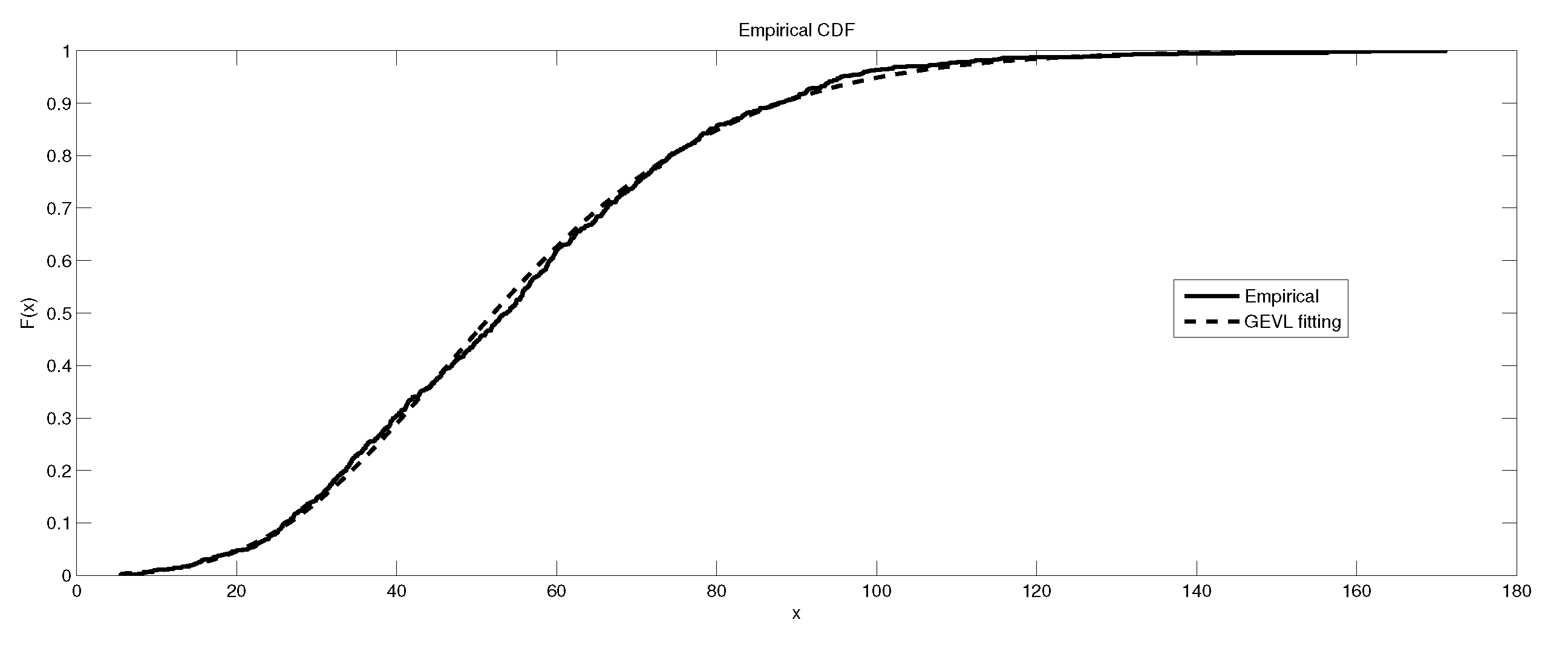
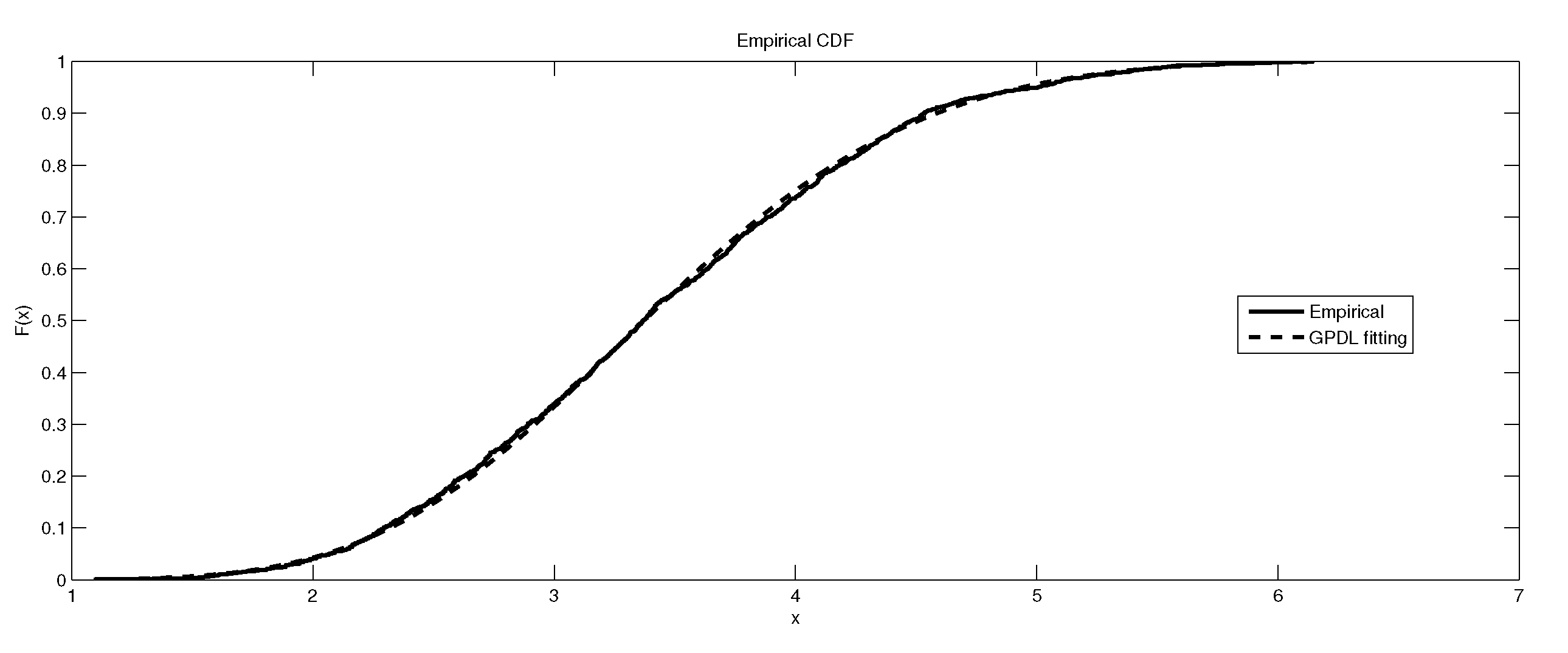
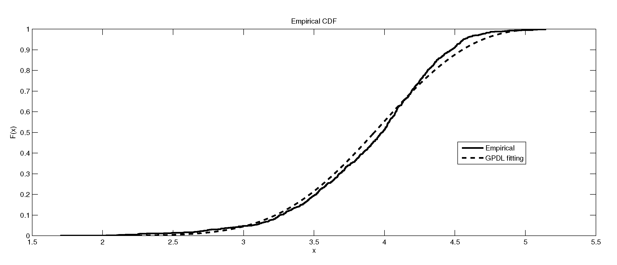
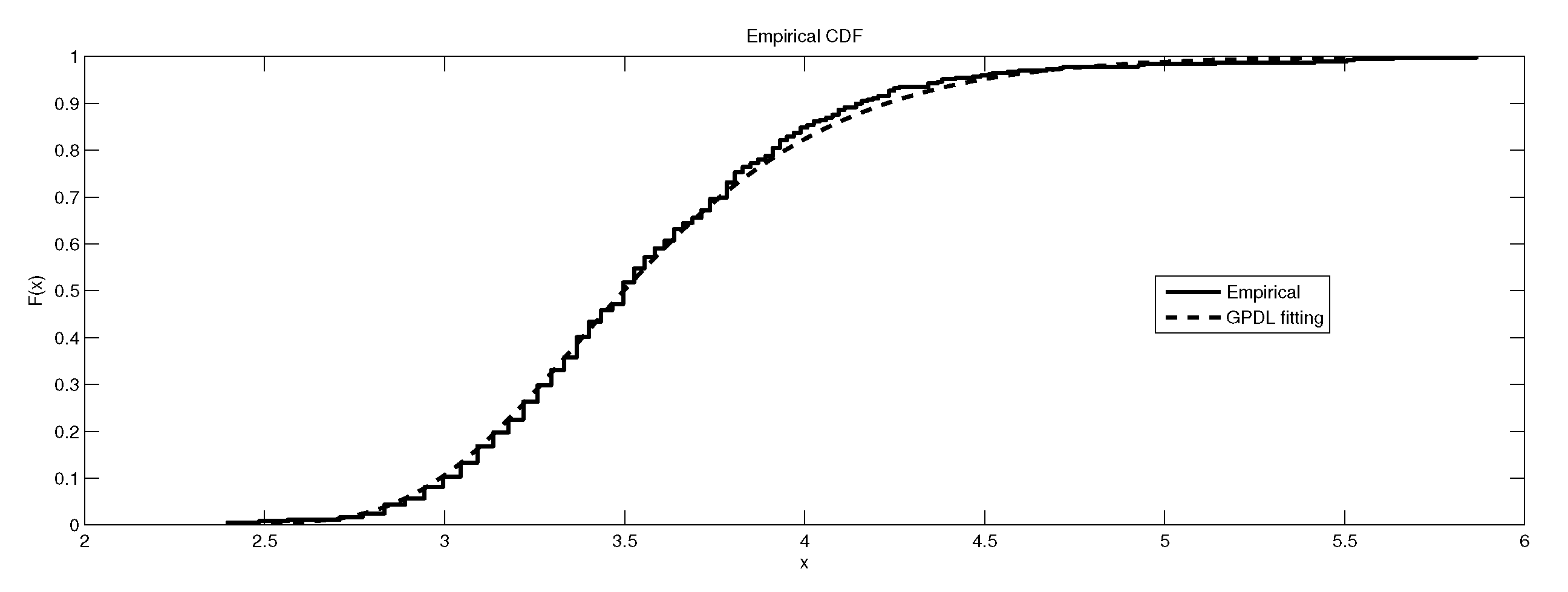
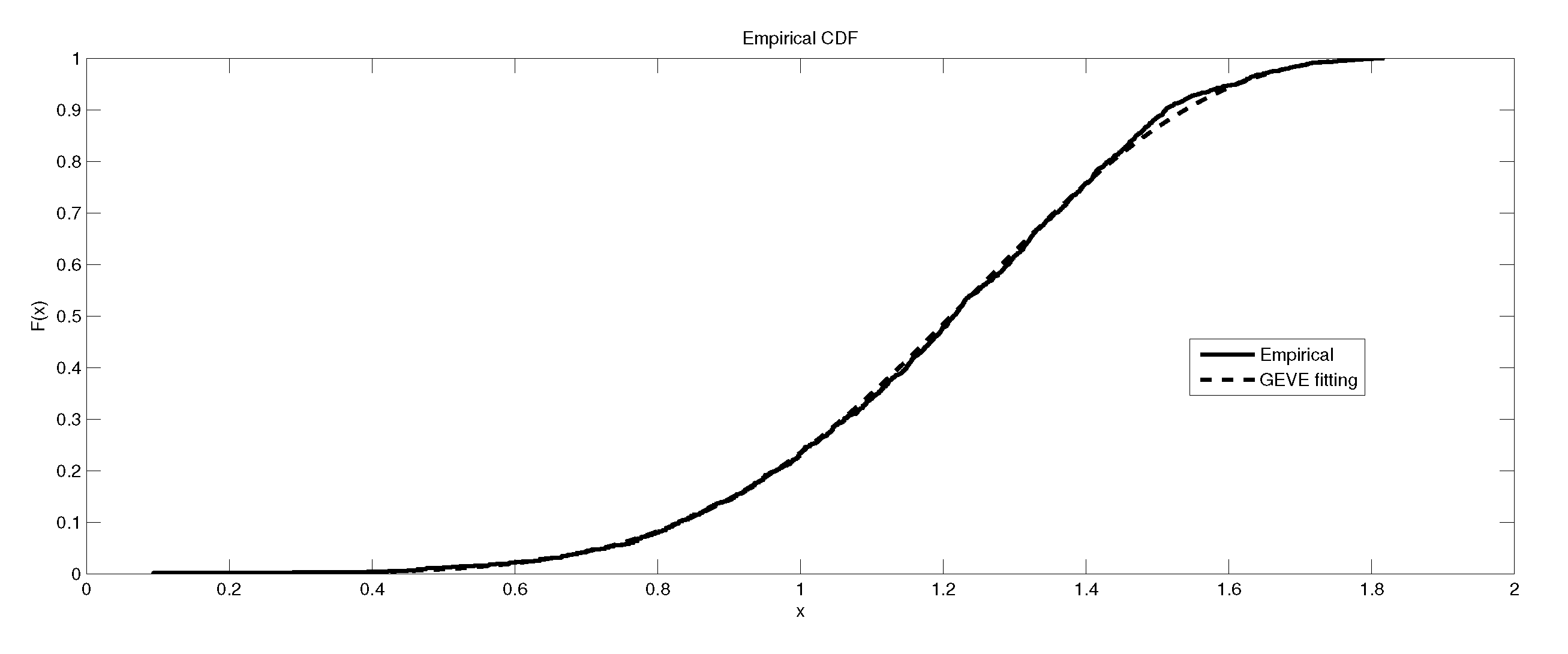
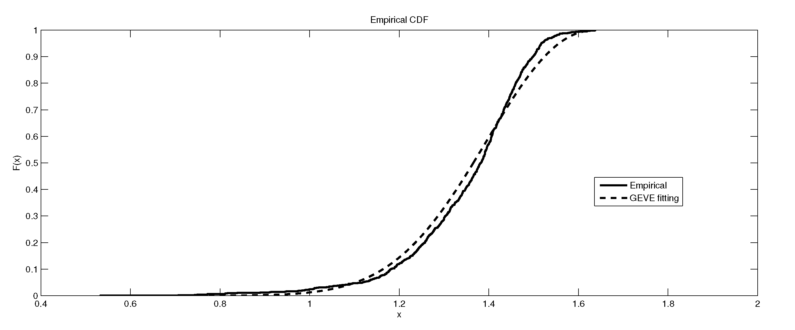
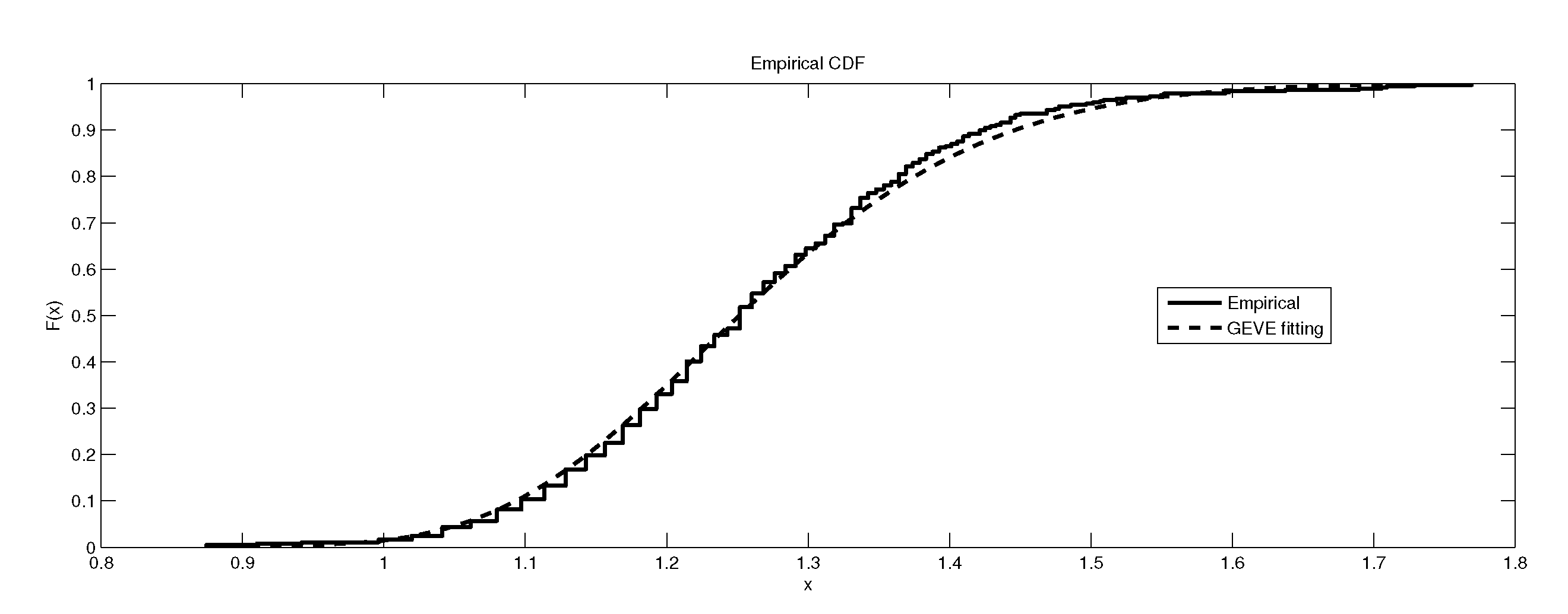
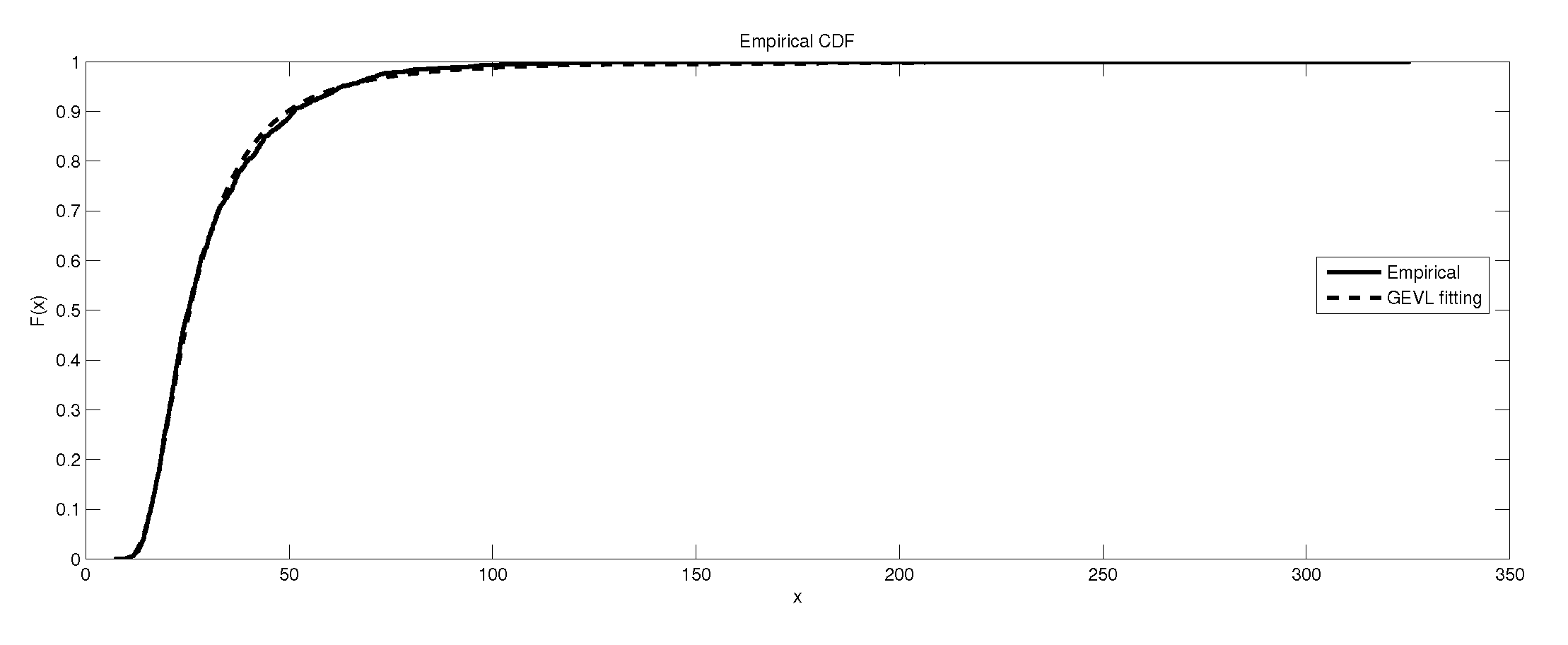
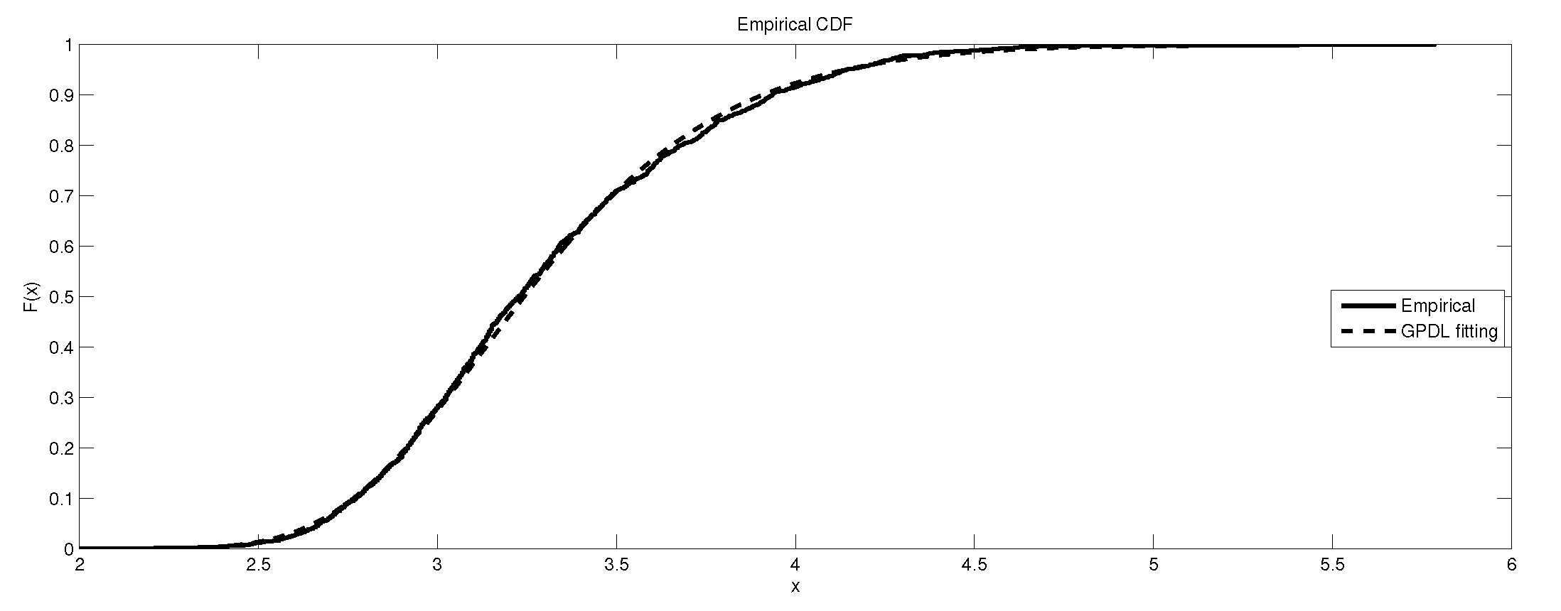
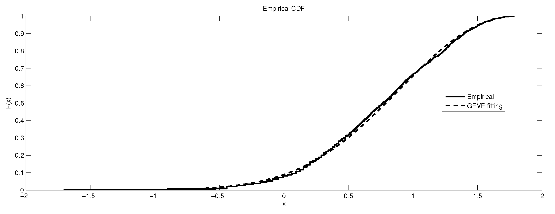
$PM10$	0.4131	0.0342	accept $H_0$

gives the result of the Kolmogorov–Smirnov (K-S) test for fitting the three models $G(x;\mu ,\sigma ,\gamma ),$$P_{1;\gamma }(x;a,b)$, and $W_{1;\gamma }(x;a,b)$ to the maximum data sets from LB6.

Table 7. Summary statistics for maximum data from GR4.

	n	Minimum	Maximum	Median	Mean	SD	Skewness	Kurtosis
$NO$	1706	1.2	380.60	8.6	23.265	39.721	4.043	21.225
$N{O}_2$	1706	4.3	120.6	34.6	36.82	17.8640	0.6906	0.5265
$PM10$	1471	7.4	325.29	25.2	30.529	18.527	4.7380	53.16945

illustrates the summary statistics for these maximum data set. Finally, the graphical representations of the data sets and the fitted distributions are given in Figure 1, Figure 2, Figure 3, Figure 4, Figure 5, Figure 6, Figure 7, Figure 8 and Figure 9.

The second data set is taken from the site Greenwich-Eltham (denoted by GR4). The daily maxima of these pollutants are recorded every hour, so around 43,825 records are presented from 1 January 2014 to 31 December 2018. These data are publicly available from the following site: http://www.londonair.org.uk/london/asp/datadownload.asp.

Table 8. Estimate parameters of the generalized extreme value distributions for GR4.

Estimate parameters of the GEVL $G(x;\mu ,\sigma ,\gamma )$ via BM approach for GR4
Pollutant	$\widehat{\gamma }$	$\widehat{\sigma }$	$\widehat{\mu }$
$NO$	1.0065	5.6233	6.1006
$N{O}_2$	−0.0537	14.9302	28.8916
$PM10$	0.3007	8.5229	22.2351
Parameter estimations of the GEVP $P_{1;\gamma }(x;a,b)$ via BM approach for GR4
Pollutant	$\widehat{\gamma }$	$\widehat{b}$	$\widehat{a}$
$NO$	−0.0013	1.0922	0.1334
$N{O}_2$	−0.3830	1.7425	0.0031
$PM10$	−0.0739	2.5652	$3.51\times {10}^{-4}$
Estimate parameters of the GEVE $W_{1;\gamma }(x;a,b)$ via BM approach for GR4
Pollutant	$\widehat{\gamma }$	$\widehat{b}$	$\widehat{a}$
$NO$	−0.4550	1.7980	0.3384
$N{O}_2$	−0.4795	5.4804	0.0015
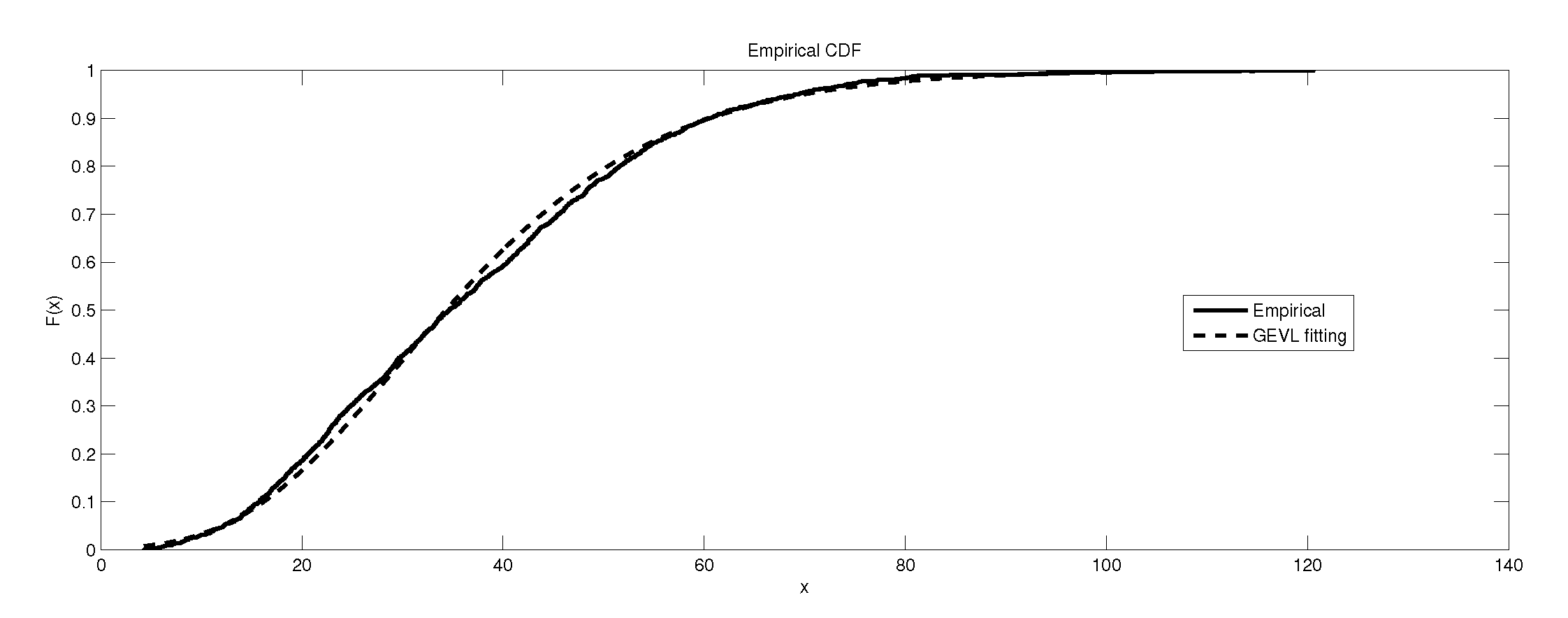
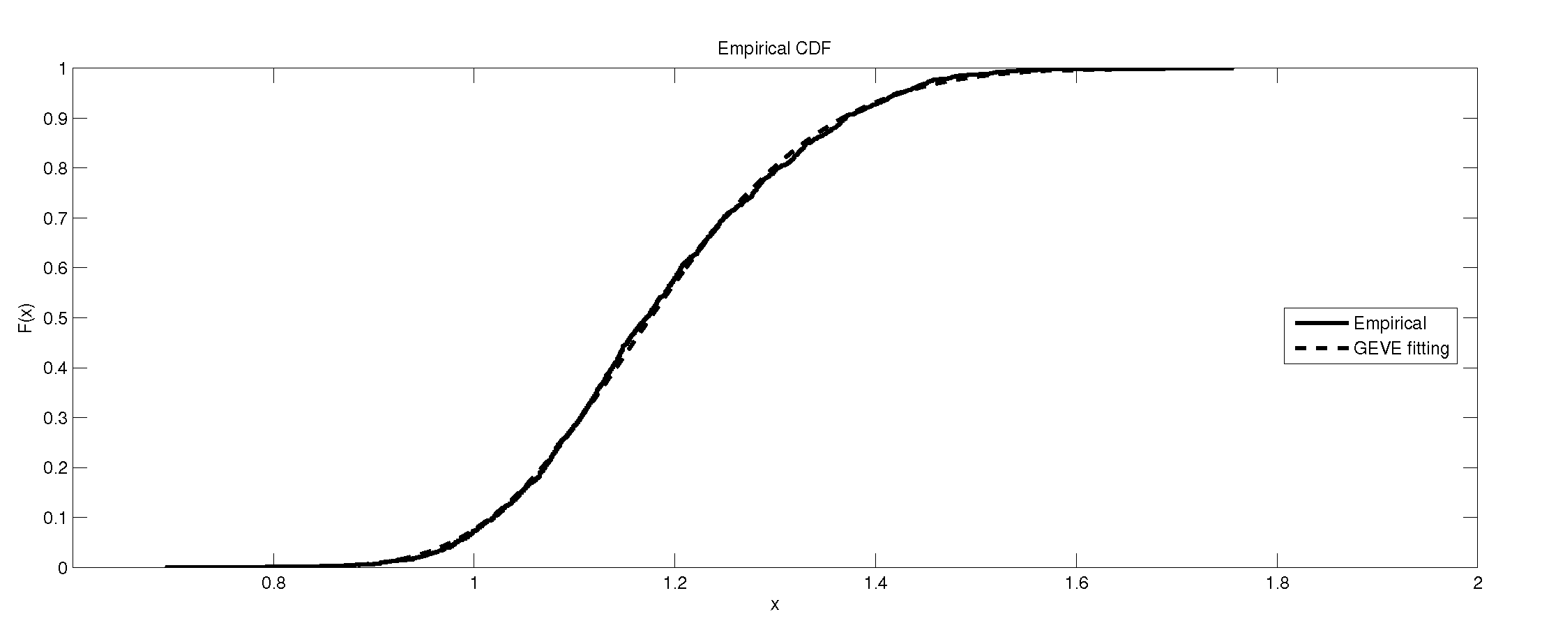
$PM10$	−0.1741	7.8801	$1.352\times {10}^{-4}$

is devoted to the estimate parameters of the generalized extreme value distributions for GR4.

Table 9. K-S test for the maximum data from GR4.

Fitting data of GR4 by the GEVL $G(x;\widehat{\mu },\widehat{\sigma },\widehat{\gamma })$
Pollutant	P	$KSSTAT$	Decision
$NO$	0.0086	0.0398	reject $H_0$
$N{O}_2$	0.0184	0.0370	reject $H_0$
$PM10$	0.2332	0.0269	accept $H_0$
Fitting data of GR4 by the GEVP $P_{1;\widehat{\gamma }}(x;\widehat{a},\widehat{b})$
Pollutant	P	$KSSTAT$	Decision
$NO$	0.0061	0.0386	reject $H_0$
$N{O}_2$	0.0098	0.0367	reject $H_0$
$PM10$	0.1073	0.0274	accept $H_0$
Fitting data of GR4 by the GEVE $W_{1;\widehat{\gamma }}(x;\widehat{a},\widehat{b})$
Pollutant	P	$KSSTAT$	Decision
$NO$	0.0817	0.0270	accept $H_0$
$N{O}_2$	$4.496\times {10}^{-4}$	0.0474	reject $H_0$
$PM10$	0.1752	0.0242	accept $H_0$

gives the result of the Kolmogorov–Smirnov (K-S) test for fitting the three models $G(x;\mu ,\sigma ,\gamma ),$$P_{1;\gamma }(x;a,b)$ and $W_{1;\gamma }(x;a,b)$ to the maximum data sets from GR4. Finally, the graphical representations of the data set and the fitted distributions are given in Figure 10, Figure 11, Figure 12, Figure 13, Figure 14, Figure 15, Figure 16, Figure 17 and Figure 18.

The result summary of this study is given below, where the more favorable model is chosen among accepted models and has a minimum KSSTAT value.

• Only the power and exponential models are favorable in describing the pollutant $NO$ that is monitored by LB6. The power model is the best one.
• The linear model is only the favorable model to describe the pollutant $N{O}_2$ that is monitored by LB6.
• All of the models are favorable to describe the pollutant $PM10$ that is monitored by LB6. The best model is the linear model followed by the power model.
• Only the e-model is favorable to describe the pollutant $NO$, which is monitored by GR4.
• None of the three models is favorable to describe the pollutant $N{O}_2$ that is monitored by GR4.
• All of the models are favorable to describe the pollutant $PM10$ that is monitored by GR4. The best model is the e-model followed by the linear model.

It is worth remarking that the study shows an interesting fact that the kurtosis of the data has an impact, to some extent, on the kind of the extreme model that describes the data, e.g., as the kurtosis increases, the e-model becomes more favorable. Moreover, the linear, power and exponential models become less favorable to fit the symmetric-platykurtic data set (for details about the description of data according to the skewness and kurtosis, see [24,25]), e.g., the case of pollutant $N{O}_2.$ Finally, a quick look at the Figure 1, Figure 2, Figure 3, Figure 4, Figure 5, Figure 6, Figure 7, Figure 8, Figure 9, Figure 10, Figure 11, Figure 12, Figure 13, Figure 14, Figure 15, Figure 16, Figure 17 and Figure 18 reveals that the curves of the empirical DF and the tested family nearly coincide when we accept $H_0$ (e.g., Figure 2, Figure 3 and Figure 4, Figure 6, Figure 7, Figure 9, Figure 12, Figure 15, Figure 16, and Figure 18), while, in the case of the rejection, the two curves diverge in some regions. This result endorses the results that are given in Table 6 and Table 9.

6. Conclusions

In this paper, we developed the EVT under exponential normalization to model extreme values, which are arisen in different natural phenomena. An estimate of the shape parameter of the generalized value distributions that related to the EVT under exponential normalization was proposed. New four generalized Pareto distributions related to the EVT under exponential normalization are obtained and their properties are elucidated. Estimates for the extreme value index of these distributions are suggested. The linear, power, and the suggested exponential models were applied, with a comparison, to several real data sets. The comparison between the three models revealed that the skewness and kurtosis of the data have an impact on the kind of the extreme model that describes the data.

References

- Barakat, H.M.; Nigm, E.M.; Khaled, O.M. Statistical Techniques for Modelling Extreme Value Data and Related Applications; Cambridge Scholars Publishing: Newcastle upon Tyne, UK, 2019. [Google Scholar]
- Galambos, J. The Asymptotic Theory of Extreme Order Statistics, 2nd ed.; Wiley: New York, NY, USA, 1987. [Google Scholar]
- Balkema, A.A.; de Haan, L. Residual life time at great age. Ann. Probab. 1974, 2, 792–804. [Google Scholar] [CrossRef]
- Pickands, J. Statistical inference using extreme order statistics. Ann. Stat. 1975, 3, 119–131. [Google Scholar]
- Pancheva, E. Limit theorems for extreme order statistics under nonlinear normalization. In Stability Problems for Stochastic Models; Lecture Notes in Math.; Springer: Berlin/Heidelberg, Germany, 1984. [Google Scholar]
- Barakat, H.M.; Nigm, E.M.; El-Adll, E.M. Comparison between the rates of convergence of extremes under linear and under power normalization. Stat. Pap. 2010, 51, 149–164. [Google Scholar] [CrossRef]
- Nasri-Roudsari, D. Limit distributions of generalized order statistics under power normalization. Commun. Stat. Theory Methods 1999, 28, 1379–1389. [Google Scholar] [CrossRef]
- Barakat, H.M.; Nigm, E.M.; Khaled, O.M. Extreme Value Modeling under Power Normalization. Appl. Math. Model. 2013, 37, 10162–10169. [Google Scholar] [CrossRef]
- Barakat, H.M.; Nigm, E.M.; Khaled, O.M. Statistical modeling of extremes under linear and power normalizations with applications to air pollutions. Kuwait J. Sci. Eng. 2014, 41, 1–19. [Google Scholar]
- Barakat, H.M.; Nigm, E.M.; Khaled, O.M.; Khan, F.M. Bootstrap order statistics and modeling study of the air pollution. Commun. Stat.-Simul. Comput. 2015, 44, 1477–1491. [Google Scholar] [CrossRef]
- Barakat, H.M.; Nigm, E.M.; Khaled, O.M.; Alaswed, H.A. The counterparts of Hill estimators under power normalization. J. Appl. Stat. Sci. 2016, 22, 87–98. [Google Scholar]
- Barakat, H.M.; Nigm, E.M.; Alaswed, H.A. The Hill estimators under power normalization. Appl. Math. Model. 2017, 45, 813–822. [Google Scholar] [CrossRef]
- Barakat, H.M.; Nigm, E.M.; Khaled, O.M.; Alaswed, H.A. The estimations under power normalization for the tail index, with comparison. AStA Adv. Stat. Anal. 2018, 102, 431–454. [Google Scholar] [CrossRef]
- Subramanya, U.R. On max domains of attraction of univariate p-max stable laws. Stat. Probab. Lett. 1994, 19, 271–279. [Google Scholar] [CrossRef]
- Christoph, G.; Falk, M. A note on domains of attraction of p-max stable laws. Stat. Probab. Lett. 1996, 28, 279–284. [Google Scholar] [CrossRef]
- Sreehari, M. General max-stable laws. Extremes 2009, 12, 187–200. [Google Scholar] [CrossRef]
- Pancheva, E. Max-semistability: A survey. ProbStat Forum 2010, 3, 11–24. [Google Scholar]
- Barakat, H.M.; Omar, A.R.; Khaled, O.M. A new flexible extreme value model for modeling the extreme value data, with an application to environmental data. Stat. Probab. Lett. 2017, 130, 25–31. [Google Scholar] [CrossRef]
- Ravi, S.; Mavitha, T.S. New limit distributions for extreme under a nonlinear normalization. PropStat Form 2016, 9, 1–20. [Google Scholar]
- Barakat, H.M.; Nigm, E.M.; Abo Zaid, E.O. Asymptotic distributions of record values under exponential normalization. Bull. Belg. Math. Soc. Simon Stevin 2019, 26, 743–758. [Google Scholar] [CrossRef]
- Alyousifi, Y.; Othman, M.; Sokkalingam, R.; Faye, I.; Silva, P.C.L. Predicting Daily Air Pollution Index Based on Fuzzy Time Series Markov Chain Model. Symmetry 2020, 12, 293. [Google Scholar] [CrossRef] [Green Version]
- Zhou, S.; Deng, Q.; Liu, W. Extreme air pollution events: Modeling and prediction. J. Cent. South Univ. 2012, 19, 1668–1672. [Google Scholar] [CrossRef]
- Marlier, M.E.; Amir, S.J.; Kinney, P.L.; DeFries, R.S. Extreme Air Pollution in Global Megacities. Curr. Clim. Chang. Rep. 2016, 2, 15–27. [Google Scholar] [CrossRef] [Green Version]
- Barakat, H.M. A new method for adding two parameters to a family of distributions with application to the normal and exponential families. Stat. Methods Appl. (SMA) 2015, 24, 359–372. [Google Scholar] [CrossRef]
- Barakat, H.M.; Khaled, O.M. Towards the establishment of a family of distributions that best fits any data set. Comm. Statis.-Sim. Comput. 2017, 46, 6129–6143. [Google Scholar] [CrossRef]
Figure 1.
The depiction of the data set of and the fitted GEVL for LB6.
Figure 2.
Figure 3.
Figure 4.
The depiction of the data set of and the fitted GEVP for LB6.
Figure 5.
Figure 6.
Figure 7.
The depiction of the data set of and the fitted GEVE for LB6.
Figure 8.
Figure 9.
Figure 10.
The depiction of the data set of and the fitted GEVL for GR4.
Figure 11.
Figure 12.
Figure 13.
The depiction of the data set of and the fitted GEVP for GR4.
Figure 14.
Figure 15.
Figure 16.
The depiction of the data set of and the fitted GEVE for GR4.
Figure 17.
Figure 18.