An LMI Approach to Nonlinear State-Feedback Stability of Uncertain Time-Delay Systems in the Presence of Lipschitzian Nonlinearities

Abstract

This article proposes a new nonlinear state-feedback stability controller utilizing linear matrix inequality (LMI) for time-delay nonlinear systems in the presence of Lipschitz nonlinearities and subject to parametric uncertainties. Following the Lyapunov–Krasovskii stabilization scheme, the asymptotic stability criterion resulted in the LMI form and the nonlinear state-feedback control technique was determined. Due to their significant contributions to the system stability, time delays and system uncertainties were taken into account while the suggested scheme was designed so that the system’s stabilization was satisfied in spite of time delays and system uncertainties. The benefit of the proposed method is that not only is the control scheme independent of the system order, but it is also fairly simple. Hence, there is no complexity in using the proposed technique. Finally, to justify the proficiency and performance of the suggested technique, a numerical system and a rotational inverted pendulum were studied. Numerical simulations and experimental achievements prove the efficiency of the suggested control technique.

1. Introduction

Time delays are usually encountered in numerous industrial systems that must be controlled, such as distributed networks, chemical processes, telecommunications, electrical servo systems, and nuclear reactors, etc. [1,2,3,4]. Because states of the system depend on the present time and a time period in the past, time delays occur in dynamical systems, and ignoring their effect yields severe deterioration in system performance or even system instability [5,6]. Thus, control of time-delay systems is known to have practical significance [7,8,9]. Recent decades have observed a widespread attention given to the synthesis of appropriate control laws for time-delay dynamical systems in the presence of parameter uncertainties [10,11,12]. In [13], an adaptive fuzzy backstepping technique was proposed for the nonlinear dynamical systems with unmeasured states and unknown time delays. In [14], H_∞ stabilization control for the time-delay Takagi–Sugeno fuzzy systems under nonlinear perturbations and sampled-data input was investigated. By using output feedback, the authors of [15] studied the robust stabilization problem of a class of time-varying time-delay dynamical systems, which were not perfectly known, where the system output was modeled through a nonlinear function depending on the delayed inputs and states. In [16], the state-feedback stability control of switched discrete-time singular systems in the presence of time-varying state delays was presented. In [17], the stabilization problem of nonlinear cascade time-delay systems using the converse Lyapunov stabilization and invariant set theories was presented.

From a practical point of view, most process models, including power systems [18], robotic manipulators [19], non-holonomic systems [20], and flexible space structures [21], suffer from system uncertainties. Thus, system uncertainties should always be taken into account when a control system for both stability and performance is designed. The design of a robust nonlinear state-feedback control scheme that overcomes system uncertainties has been the subject of substantial investigation over the years. The linear matrix inequality (LMI) approach is a suitable and strong technique to deal with system uncertainties including parametric [22] or unstructured uncertainties [23]. Due to its influential structure, the LMI technique has been widely applied to obtain solutions for convex problem minimization, such as H_∞ control [24] and H₂ control [25]. Dealing with difficult problems for which there is no analytical solution is another significant feature of the LMI approach that attracts the attention of many researchers since it offers numerically tractable means [26,27]. Furthermore, powerful algorithms exist, such as interior-point ones, to provide a way of dealing with LMI problems. Two robust H_∞ state-feedback controllers based on LMIs for time-delay discrete-time systems and uncertain switched impulsive linear systems were proposed in [28] and [29], respectively. In [30], a robust H_∞ fuzzy-logic controller for Takagi–Sugeno time-delay bilinear discrete-time systems in the presence of disturbances was presented in which the stabilization conditions were formulated as LMI. A combination of Lyapunov parameter-dependent function and LMI was also used in [31,32] to develop a control scheme for uncertain systems subject to time delay. Moreover, based on the LMI approach, the problem of stabilization of a uniform Euler–Bernoulli beam and a two-dimensional Burgers’ equation have been investigated in [33] and [34], respectively. To the best of the authors’ knowledge, little consideration has been drawn to the problem of nonlinear state-feedback stability for nonlinear time-delay systems with Lipschitz nonlinearities via LMIs.

This work aimed to present a state-feedback controller for the stabilization of Lipschitz nonlinear systems. Time delays and parametric uncertainties were also taken into account due to their significant contribution to the system stability. Using a Lyapunov–Krasovskii functional, some asymptotic stability conditions were formed as LMI and the parameters of the state-feedback controller were found through LMI. The offered control law ensures asymptotic stabilization of the systems, even if the nonlinear function is not equal to zero. Unlike the previous investigations, the LMI conditions possess fewer pre-assumed design parameters, and thus, the designed method may lead to less conservative conditions. Moreover, the control scheme is independent of the order of systems’ model. The chief novelties of the planned technique are presented as follows:

-

Design of a nonlinear state-feedback stabilizing controller for nonlinear systems in the presence of time delays, Lipschitz nonlinearity, and parametric uncertainties.

-

Achievement of asymptotic stabilization based on the Lyapunov–Krasovskii stabilization theory and the LMI approach.

-

The suggested control scheme is rather straightforward; there is no difficulty in the employment of this technique.

-

Application of the offered method on a nonlinear unstable system and a rotational inverted pendulum to prove the efficiency of the method.

The presentation of this work is as follows: Section 2 gives the definition of the problem and required preliminaries. Section 3 presents the stability analysis and design process of the LMI-based nonlinear state-feedback control law for the time-delay systems in the presence of uncertainties and nonlinearities. In Section 4, some simulation and experimental results are illustrated. Finally, Section 5 concludes the paper.

2. Problem Description

Consider the uncertain time-delay system as

$$\begin{array}{ll}\dot{x}(t)& =f(x)+(A+\Delta A)x(t)+A_{1}x(t-\tau )+(B+\Delta B)u(t),\\ y(t)& =Cx(t),\end{array}$$

(1)

where $\tau \in R$, $u(t)\in R^n$, $y(t)\in R^p$, and $x(t)\in R^n$ represent the time delay, control inputs, outputs, and states of the system, respectively. The matrices $A$, $A_1$, $B$, and $C$ are constant matrices with suitable dimensions; the nonlinear function $f(x)\in R^n$ is a time-varying vector; $\Delta A$ and $\Delta B$ signify the parametric uncertainties.

Lemma 1.

For any real$\gamma >0$, the following inequality is satisfied [35]:

$$A^{T}B+B^{T}A\le \gamma A^{T}A+\frac{1}{\gamma }{B}^{T}B$$

(2)

where the matrices A and B are of consistent dimensions.

Lemma 2 (Schur Complement) [36].

Consider the symmetric block matrix$\Pi =\left[\begin{array}{cc}A& B\\ B^T& D\end{array}\right]$, where$A=A^T$and$D=D^T$, the condition$\Pi <0$is equivalent to$D<0$and${\Gamma }_D=A-B{D}^{-1}{B}^T<0$. Similarly, the condition$\Pi <0$is equivalent to$A<0$and${\Gamma }_A=D-B^T{A}^{-1}B<0$.

Assumption 1.

$f(x)$is a Lipschitzian nonlinear function for all$x\in R^n$and$\overline{x}\in R^n$satisfying [37]:

$$\Vert f(x)-f(\overline{x})\Vert \le L\Vert (x-\overline{x})\Vert ,$$

(3)

where$L\in R^{n\times n}$is a constant Lipschitz matrix. The inequality (3) can be written as

$${(f(x)-f(0))}^{T}I(f(x)-f(0))\le x^T{L}^{T}Lx.$$

(4)

The state-feedback controller law is designed as

$$u(t)=Fx(t)-B^{-1}f(0),$$

(5)

where$F$denotes the state-feedback gain and additional term$B^{-1}f(0)$is necessary to deal with systems possessing$f(0)\ne 0$.

Remark 1.

If$B$is a non-square and full-rank matrix, the state-feedback controller is designed utilizing the right inverse of$B$(pseudo-inverse) as:

$$u(t)=Fx(t)-B^T{(B{B}^T)}^{-1}f(0).$$

(6)

3. Nonlinear State-Feedback Stabilization

In the subsequent theorem, a sufficient condition for the stability of system (1) is presented.

Theorem 1.

Consider the uncertain nonlinear time-delay system (1) and the controller input (5). If there exist matrices$Q=Q^T>0$,$Y$, and$H$with suitable dimensions so that the LMI holds as:

$$\Gamma =\left[\begin{array}{ccccccc}\Omega & A_{1}Q& I& 0& D_A& D_B& Q\\ *& H& 0& 0& 0& 0& 0\\ *& *& -I& 0& 0& 0& 0\\ *& *& *& {\gamma }_C{B}^{-T}{E}_B^T{E}_B{B}^{-1}& 0& 0& 0\\ *& *& *& *& -{\gamma }_{A}I& 0& 0\\ *& *& *& *& *& -\frac{{\gamma }_B{\gamma }_C}{{\gamma }_B+{\gamma }_C}& 0\\ *& *& *& *& *& *& -M\end{array}\right]<0,$$

(7)

where$\Omega \triangleq AQ+Q{A}^T+BY+Y^T{B}^T+{\gamma }_B{Y}^T{E}_B^T{E}_{B}Y-H$,$M={(L^{T}L+{\gamma }_A{E}_A^T{E}_A)}^{-1}$, the parameters${\gamma }_A$,${\gamma }_B$and${\gamma }_C$are positive constants,$D_A$,$D_B$,$E_A$, and$E_B$are known constant matrices representing system uncertainties, and$P=Q^{-1}$and$P_1=Q^{-1}H{Q}^{-1}$are positive-definite matrices, then the control signal (5) guarantees the asymptotical stability of the system states and one can calculate$F$in (5) as$F=Y{Q}^{-1}$.

Proof. 

The proof of this theorem is provided in Appendix A.

Remark 2.

The notations “*”, “<”, and “$\triangleq$” denote the transpose conjugate matrix of a symmetric matrix to main diagonal, the negativeness of the real parts of all eigenvalues of the matrix, and the equivalent equality, respectively.

4. Simulation and Experimental Results

In this section, two instances are considered in order to investigate the performance of the suggested method. In the first example, an unstable nonlinear system with state delay is studied and an LMI-based controller is developed to overcome the time delay, nonlinearity, and uncertainties of the system. In the second example, the offered control approach is applied to a practical rotary inverted pendulum (RIP) system with state-delayed and nonlinear terms.

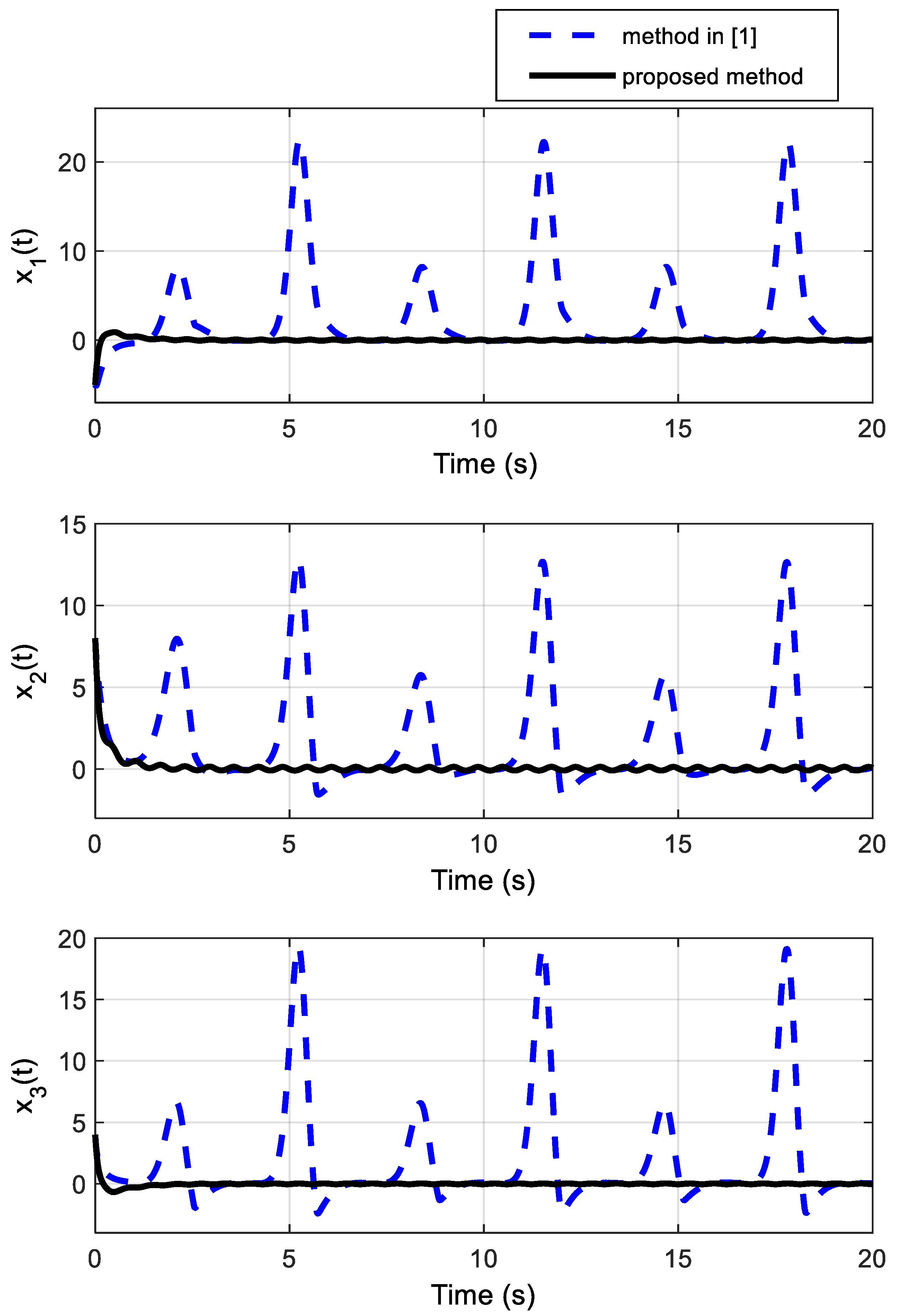
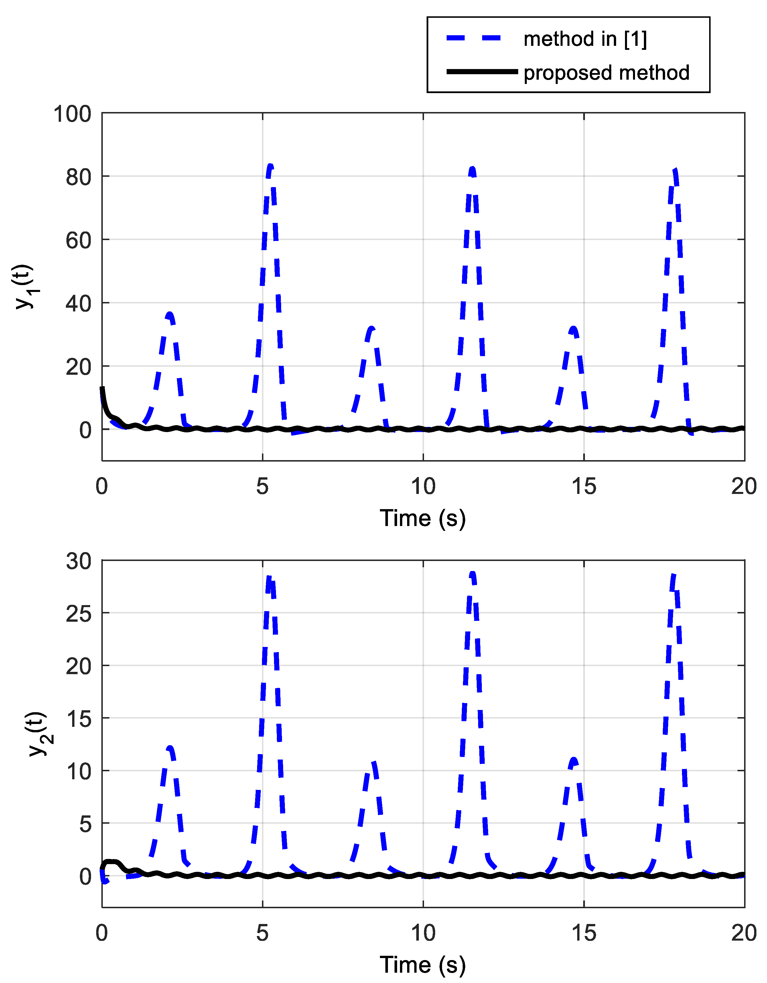
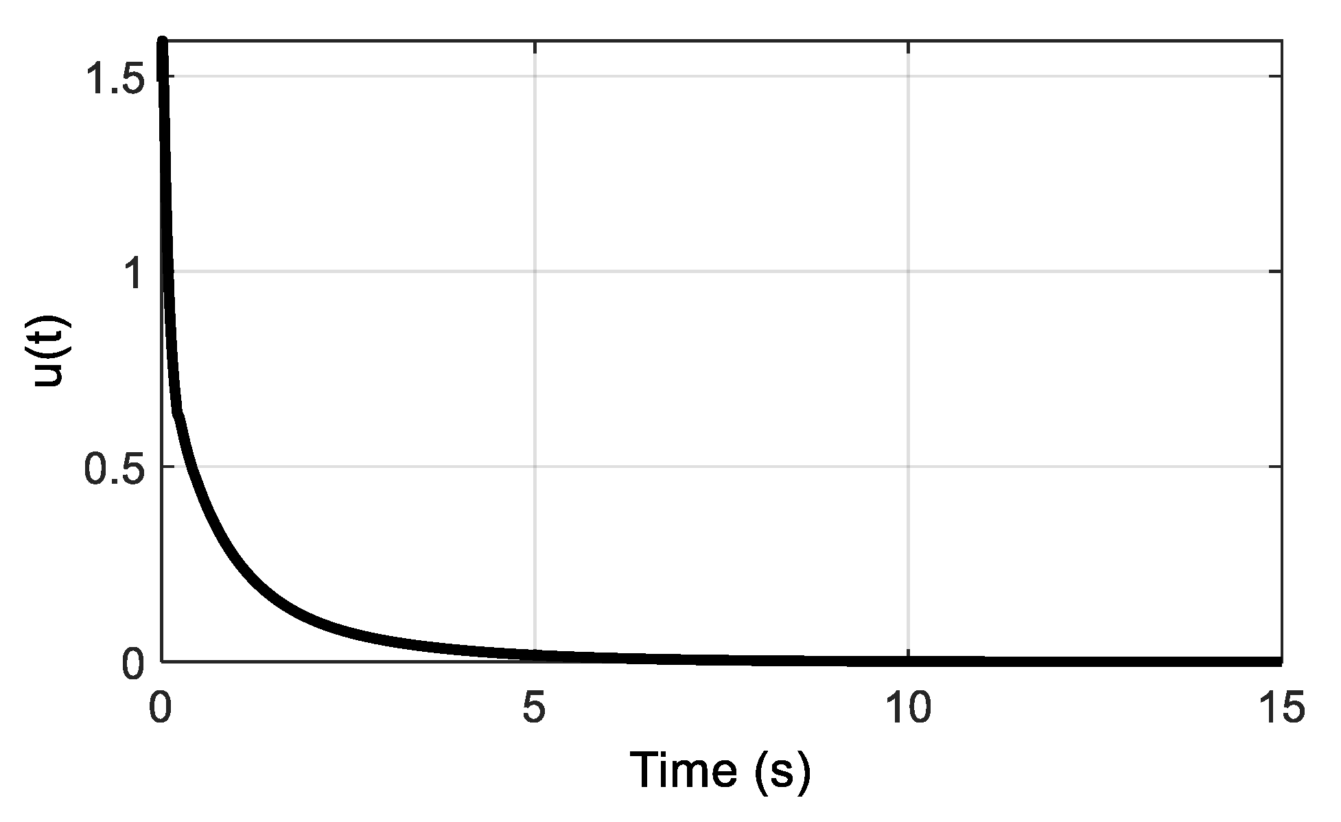
4.1. Example A: Unstable Nonlinear System

The equations of an unstable nonlinear numerical system are given by [1]:

$$\begin{array}{l}\dot{x}=\left(\begin{array}{c}0.2\cos x_1\\ 0.3\sqrt{x_2^2+5}\\ 0.4\sin x_3\end{array}\right)+\left(\begin{array}{ccc}0& 0.01& -0.01\\ 0.05& -0.04& 0\\ 0.01& 0.02& -0.03\end{array}\right)x(t-\tau )\\ +\left[\left(\begin{array}{ccc}0.1& 0.2& 0.3\\ 0.1& 0.1& -0.5\\ 0.3& -0.4& -0.3\end{array}\right)+\left(\begin{array}{ccc}0.027& 0.0345& 0.038\\ 0.02& 0.017& 0.034\\ 0.0335& 0.0325& 0.0455\end{array}\right)\sin (3t)\right]x\\ +\left[\left(\begin{array}{cccc}0.012& 0.013& 0.014& 0.016\\ 0.01& 0.014& 0.01& 0\\ 0.013& 0.017& 0.018& 0.011\end{array}\right)+\left(\begin{array}{cccc}0.0024& 0.0026& 0.0028& 0.0032\\ 0.002& 0.0028& 0.002& 0\\ 0.0026& 0.0034& 0.0036& 0.0022\end{array}\right)\cos (2t)\right]u,\\ y=\left(\begin{array}{ccc}1.5& 2& 1.25\\ 0.84& 0.5& 0.2\end{array}\right)x.\end{array}$$

(8)

Suppose that the time delay and initial conditions of the system are respectively taken as $\tau =2$, $x(0)={\left[104-6\right]}^T$. The LMI condition (7) is solved by MATLAB^® YALMIP^® solver as:

$$\begin{gathered} H=\left[\begin{array}{ccc}0.086& 0.037& 0.03\\ 0.037& 0.182& 0.042\\ 0.03& 0.042& 0.112\end{array}\right],P=\left[\begin{array}{ccc}20.63& -11.27& -12.42\\ -11.27& 33.16& -6.02\\ -12.42& -6.02& 55.46\end{array}\right], \\ {P}_1=\left[\begin{array}{ccc}51.11& -48.67& -72.99\\ -48.67& 130.36& -3.55\\ -72.99& -3.55& 298.24\end{array}\right], F=\left[\begin{array}{ccc}-95.17& 39.47& 205.77\\ -57& -86.44& -53.18\\ 105.91& 46.86& -233.61\\ -29.98& 92.37& 93.68\end{array}\right] \end{gathered}$$

Simulations of the proposed controller are given in Figure 1 and Figure 2, as compared to the simulations of [1]. For the comparison of the simulation outcomes with those of [1], system (8) is also simulated via the control input described in [1]. Figure 1 illustrates the states of system (8), which proves that the proposed control method displays faster and superior responses over those of [1]. As shown in Figure 1, the proposed method results in a more acceptable steady-state behavior of the system states in terms of accuracy.

Time responses of the outputs are presented in Figure 2, where it is indicated that the output response of [1] comprises high-frequency oscillations that are practically undesired. These simulation outcomes confirm that the suggested control scheme has superior performance in comparison with the controller of [1].

In what follows, the robustness of the proposed control technique is confirmed in a different situation. In this scenario, the new initial states are given as $x(0)={\left[\begin{array}{ccc}-5& 8& 4\end{array}\right]}^T$. Moreover, the parametric uncertainties are considered 10 times larger. Time trajectories of the states and outputs are presented in Figure 3 and Figure 4. These plots demonstrate the fast-transient responses of the recommended control scheme over the other method. The figures confirm the appropriate performance and robustness of the proposed technique in the new situation in comparison with the control method of [1].

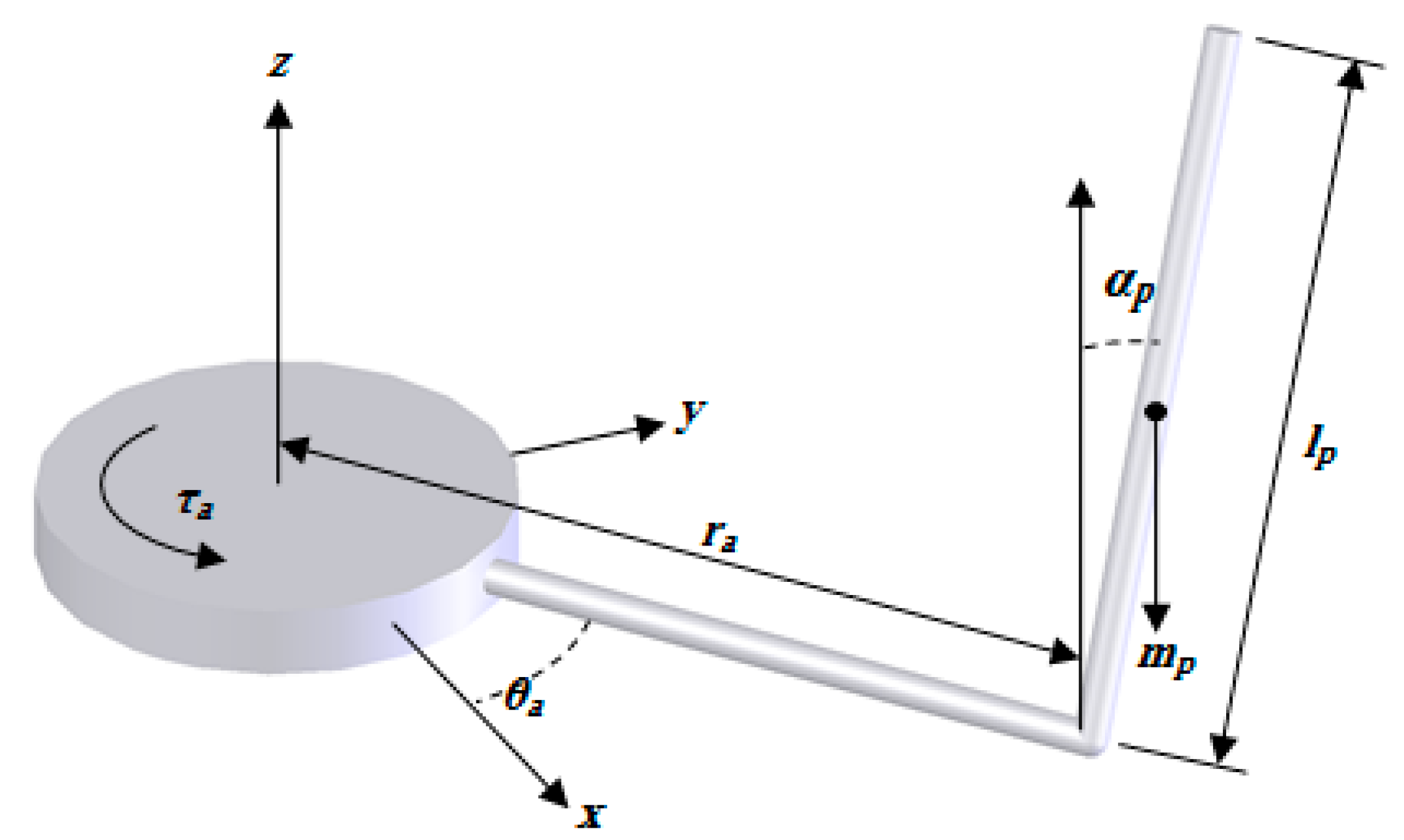
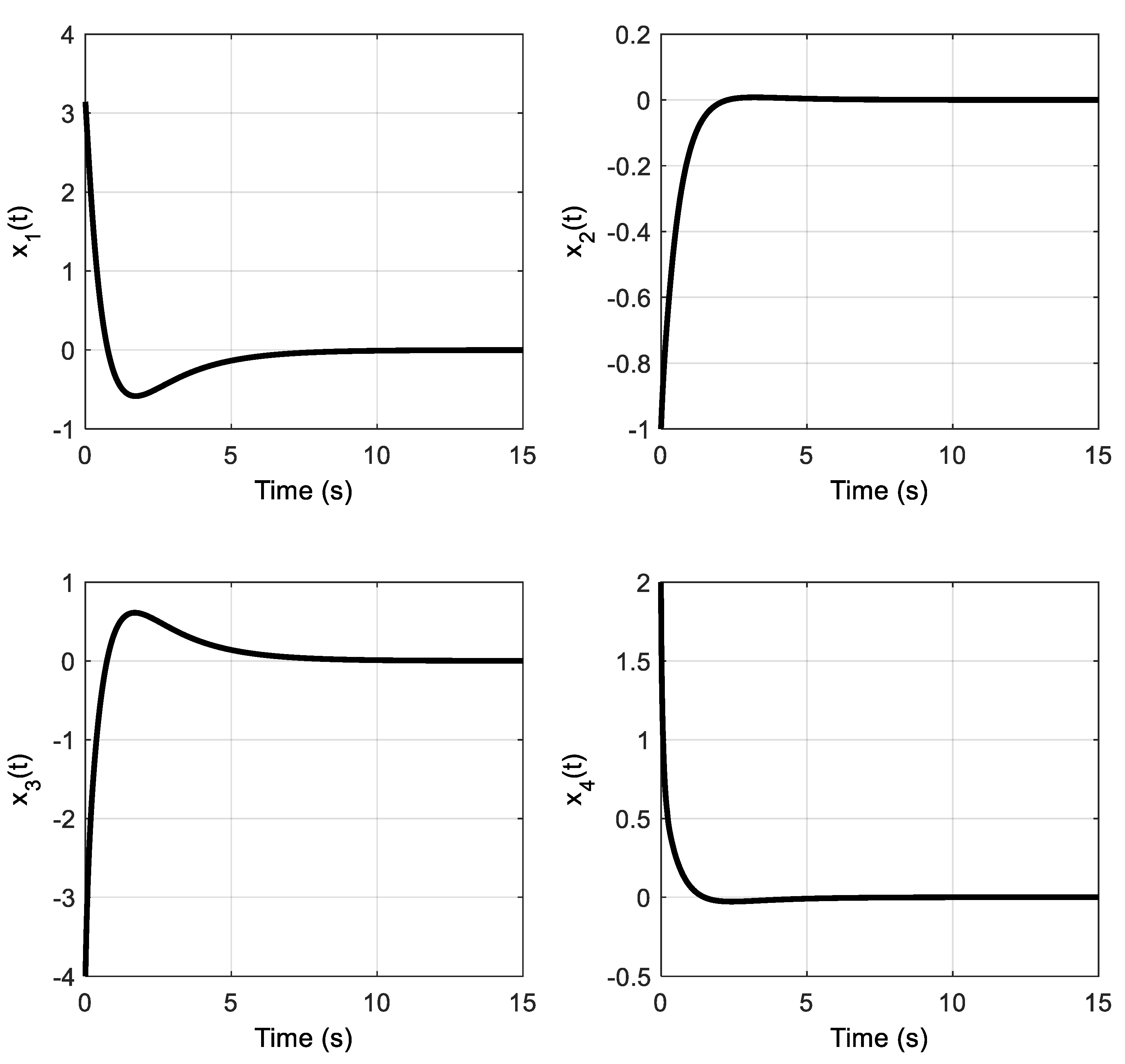
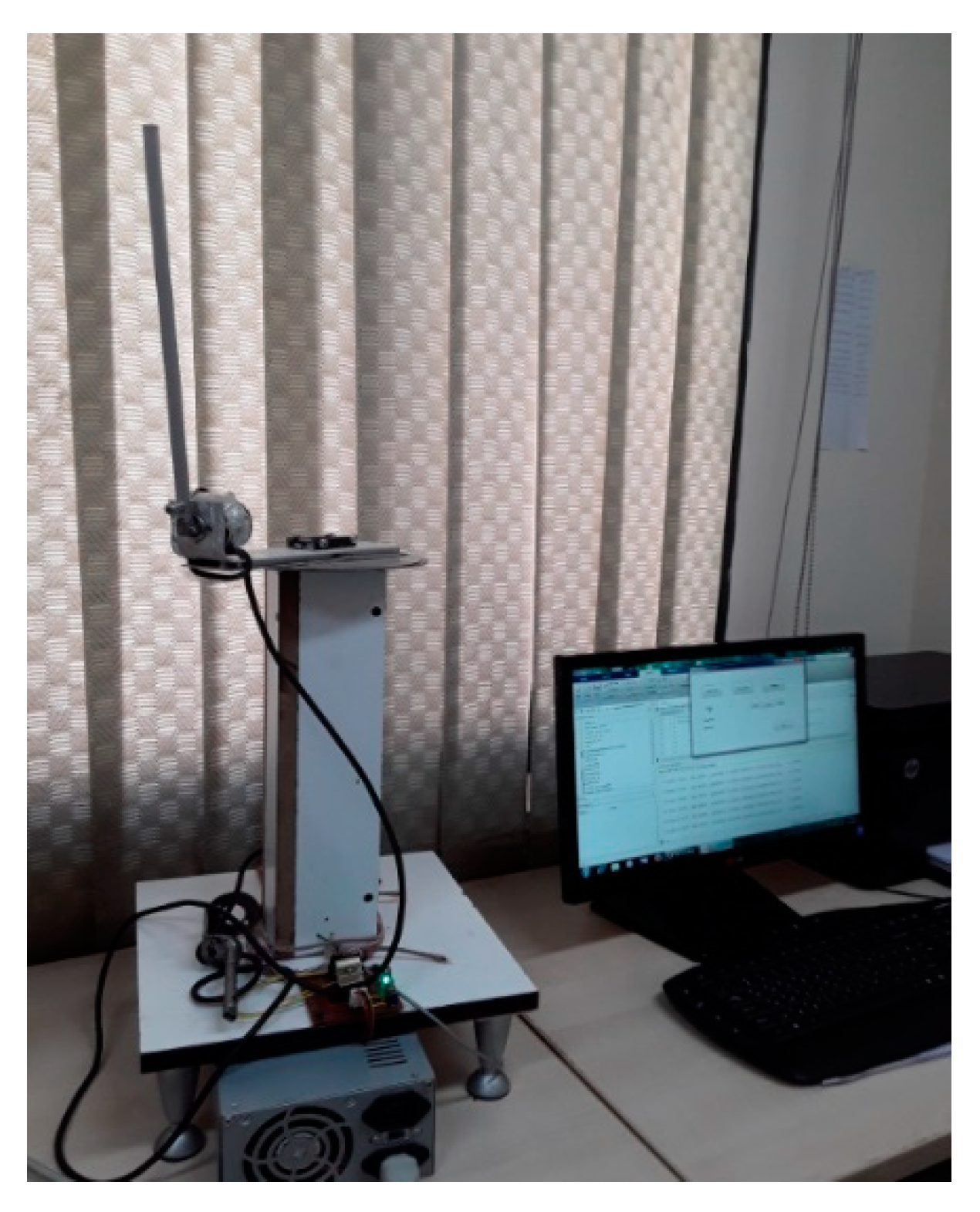
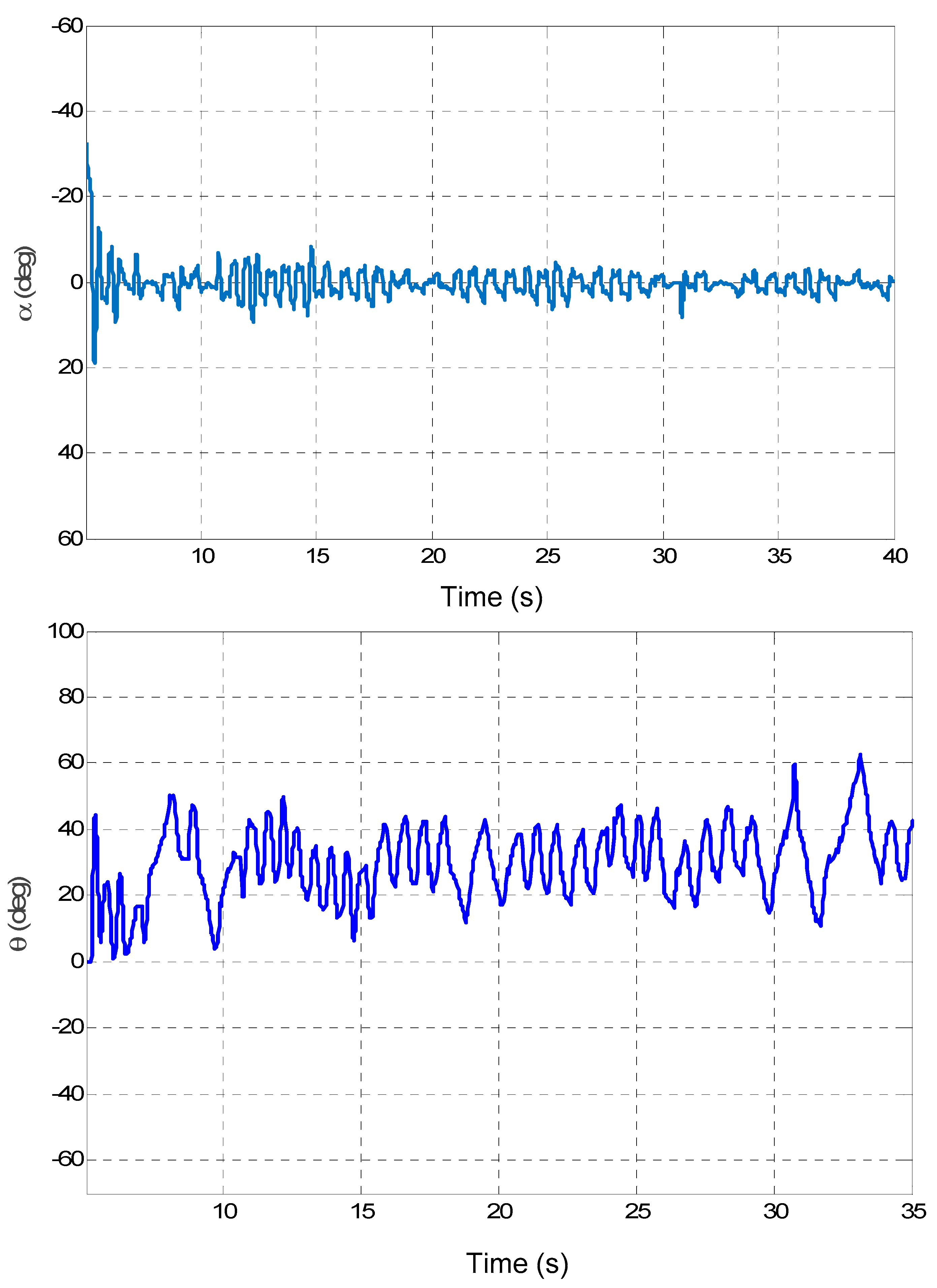
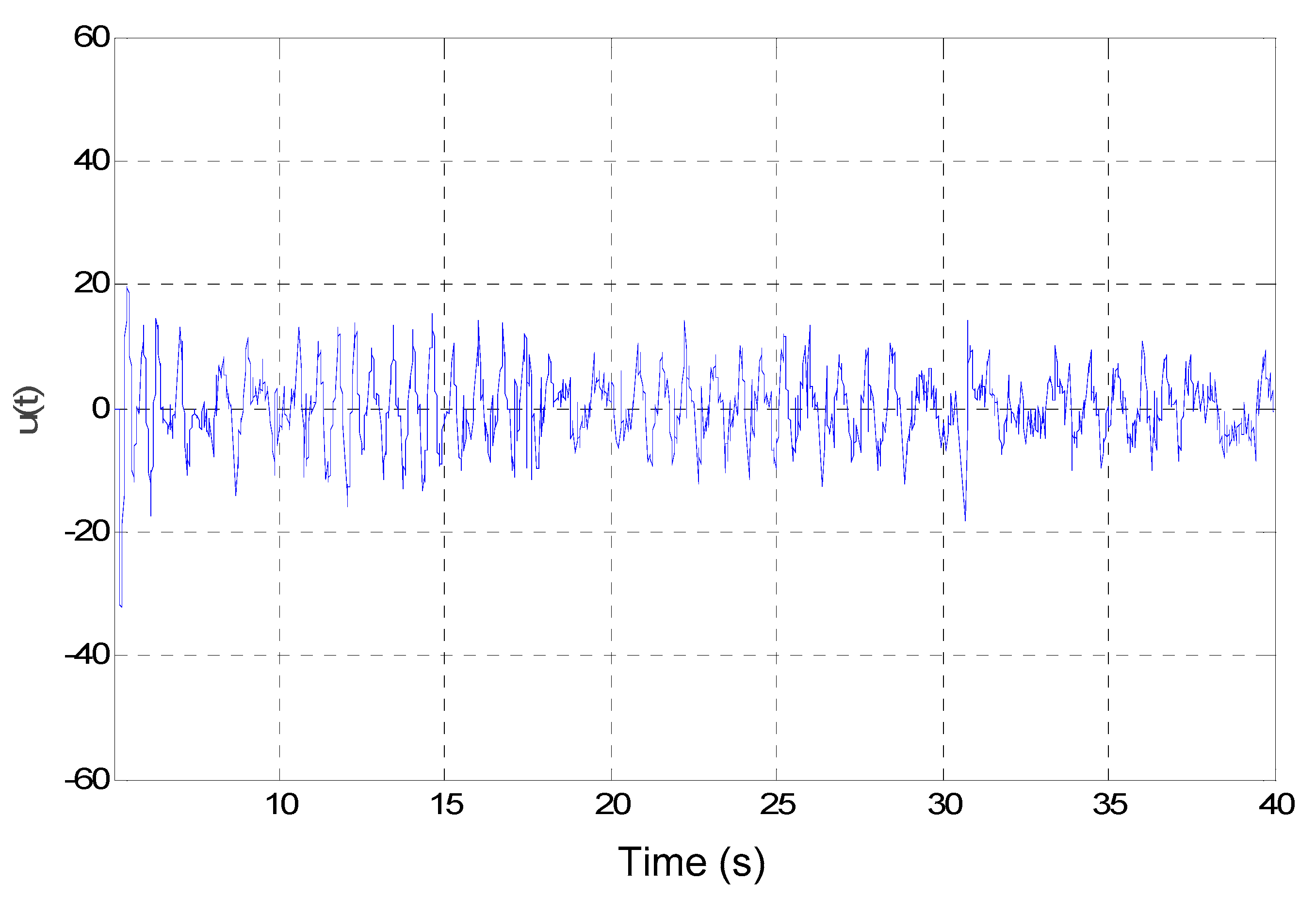
4.2. Example B: A Practical Rotational Inverted Pendulum

In the second example, we set out to balance a pendulum in an unstable upright equilibrium position in an RIP system, which is recognized as an appropriate test platform to assess the performance of various techniques. This under-actuated mechanical system has received the consideration of many investigators in various fields of study such as robotics, aerospace, marine vehicles, and pointing control. The RIP shown in Figure 5 is composed of a rotational servo-motor driving the output gear, rotational arm, and an inverted pendulum. Suppose ${\alpha }_p$, ${\theta }_a$, $m_p$, $l_p$, $r_a$, $u$, ${\tau }_a$, and $J_b$ represent the pendulum angle, arm angle, pendulum mass, pendulum length, arm length, control input, motor torque, and moment of inertia of the effective mass, respectively. The dynamics of the RIP with constant time delay, friction, and backlash effects are specified by:

$$\begin{array}{ll}{A}_p{\ddot{\theta }}_a-(C_p\sin {\alpha }_p){\dot{\alpha }}_p{}^2& +(B_p\sin 2{\alpha }_p){\dot{\alpha }}_p{\dot{\theta }}_a+F_p{\dot{\theta }}_a\\ & +G_p\mathrm{sgn}({\dot{\theta }}_a)+H_p{\theta }_a=I_{p}u+\frac{A_p{B}_p-C_p^2}{B_p}\left[\begin{array}{c}{\alpha }_p(t-\tau )\\ {\dot{\alpha }}_p(t-\tau )\\ {\theta }_a(t-\tau )\\ {\dot{\theta }}_a(t-\tau )\end{array}\right],\end{array}$$

(9)

$$B_p{\ddot{\alpha }}_p-(B_{p}sin{\alpha }_{p}cos{\alpha }_p){\dot{\theta }}_a{}^2-D_{p}sin{\alpha }_p+E_p{\dot{\alpha }}_p=0$$

(10)

where $E_p$, $F_p$, $I_p$, $H_p$, and $G_p$ are pendulum damping coefficient, arm damping constant, controller signal coefficient, elasticity constant, and arm Coulomb friction, respectively. $A_p$, $B_p$, $C_p$, and $D_p$ are considered as [38]:

$$\begin{array}{ll}{A}_p& =m_p{r}_a{}^2+J_b,\\ B_p& =\frac{1}{3}{m}_p{l}_p^2,\\ C_p& =\frac{1}{2}{m}_p{r}_a{l}_p,\\ D_p& =\frac{1}{2}{m}_{p}g{l}_p.\end{array}$$

(11)

The constants of the model (9) and (10) are set as:

$$\begin{gathered} A_p=3.291,D_p=6.052,G_p=1.428, \\ {B}_p=0.237,E_p=0.0132,H_p=1.72, \\ {C}_p=0.237,F_p=14.283,I_p=6.38. \end{gathered}$$

Therefore, the nonlinear time-delay model (9) and (10) can easily be written in the form of (1) as follows:

$$\begin{array}{l}\dot{x}=\left(\begin{array}{c}0\\ (\sin x_1\cos x_1)x_4{}^2+25.54\sin x_1\\ 0\\ (0.072\sin x_1)x_2{}^2-(0.072\sin 2x_1)x_2{x}_4-0.43\mathrm{sgn}(x_4)\end{array}\right)\\ \hspace{1em}\hspace{1em}+\left(\begin{array}{cccc}0& 1& 0& 0\\ 0& -0.056& 0& 0\\ 0& 0& 0& 1\\ 0& 0& -0.52& -4.34\end{array}\right)x+0.93\left(\begin{array}{cccc}0& 0& 0& 0\\ 0& 0& 0& 0\\ 0& 0& 0& 0\\ 1& 1& 1& 1\end{array}\right)x(t-\tau )+\left(\begin{array}{c}0.2\\ 0.1\\ 0.1\\ 1.94\end{array}\right)u,\\ y=(\begin{array}{cccc}1& 0& 0& 0\end{array})x,\end{array}$$

(12)

where $x={\left[\begin{array}{cccc}{\alpha }_p& {\dot{\alpha }}_p& {\theta }_a& {\dot{\theta }}_a\end{array}\right]}^T$. The time delay and the initial states are considered as $x(0)={\left[\begin{array}{cccc}\pi & -1& -4& 2\end{array}\right]}^T$ and $\tau =2$, respectively. Moreover, the Lipschitzian matrix is given by $L=diag(0.2,0.3,0.4,0.8).$ Using YALMIP^® solver, matrices $H$, $P$, $P_1$, $F$ are obtained as:

$$\begin{gathered} H=\left[\begin{array}{cccc}0.7213& -0.1484& 0.1765& 1.7343\\ -0.1484& 0.7503& 0.1916& 1.9435\\ 0.1765& 0.1916& 0.5853& 2.2188\\ 1.7343& 1.9435& 2.2188& 12.6601\end{array}\right], P=\left[\begin{array}{cccc}1.1107& 0.4934& 0.4132& 0.4817\\ 0.4934& 1.7864& 1.1968& -0.1674\\ 0.4132& 0.1968& 1.3576& 0.6499\\ 0.4817& -0.1674& 0.6499& 2.2046\end{array}\right]. \\ {P}_1=\left[\begin{array}{cccc}7.8512& 1.6463& 9.5245& 23.4526\\ 1.6463& 1.2598& 2.0790& 5.7018\\ 9.5245& 2.0790& 12.1973& 29.2457\\ 23.4526& 5.7018& 29.2457& 70.6682\end{array}\right], F=\left[-3.5140-3.2700-3.3280-2.0280\right]. \end{gathered}$$

The variation of the system state is illustrated in Figure 6. It is clear from this figure that the proposed approach is able to lead the system states to zero irrespective of the time delay and nonlinearities. Figure 7 indicates the required controller signal to make the states converge to zero. As a result, the robust performance of the proposed method is verified through these simulation results.

Furthermore, we performed some experiments on the practical RIP that is constructed in the Department of Electrical Engineering of University of Zanjan, Zanjan, Iran. Figure 8 shows the experimental RIP system. The angular position of the pendulum was measured using the encoder E40S (Autonics Company, Busan, Republic of Korea). The practical results for the pendulum angle, arm angle, and controller input are presented in Figure 9 and Figure 10. In the practical results, the time interval (0, 5.1) (swing-up period) is removed from the figures to focus on the control performance in the balance mode. The experimental results are similar to the simulations. This result illustrates that the offered control technique has a satisfactory and robust performance.

5. Conclusions

In this study, the problem of developing a nonlinear state-feedback controller was considered for the stabilization of time-delay nonlinear systems subject to structured uncertainties. Following the Lyapunov–Krasovskii stability theory, a nonlinear state-feedback control was derived to overcome the time delay and provide asymptotic stability of the states as well as robustness of the system against parametric uncertainties. In fact, the mentioned problem was converted into a common optimization problem that was then solved in the form of LMI. The gains of the control law were stated by the sufficient conditions via LMIs. The resultant LMI was comparatively straightforward in the computational aspect. Numerical simulation and practical outcomes were shown to approve the efficiency of the proposed approach and satisfactory outcomes were achieved. The suggested procedure can reach a promising tracking efficiency for high-order nonlinear perturbed systems. Moreover, the extension of the proposed control method based on gain-scheduled linear parameter-varying (LPV) control will be presented in future work.

References

1. Mobayen, S. Optimal LMI-based state feedback stabilizer for uncertain nonlinear systems with time-Varying uncertainties and disturbances. Complexity 2016, 21, 356–362. [Google Scholar] [CrossRef]
2. Huo, Y.; Liu, J.-B. Robust H∞ Control For Uncertain Singular Neutral Time-Delay Systems. Mathematics 2019, 7, 217. [Google Scholar] [CrossRef] [Green Version]
3. Emharuethai, C.; Niamsup, P.; Ramachandran, R.; Weera, W. Time-Varying Delayed H∞ Control Problem for Nonlinear Systems: A Finite Time Study Using Quadratic Convex Approach. Symmetry 2020, 12, 713. [Google Scholar] [CrossRef]
4. Yao, H. Anti-Saturation Control of Uncertain Time-Delay Systems with Actuator Saturation Constraints. Symmetry 2019, 11, 375. [Google Scholar] [CrossRef] [Green Version]
5. Sun, Z.-Y.; Song, Z.-B.; Li, T.; Yang, S.-H. Output feedback stabilization for high-order uncertain feedforward time-delay nonlinear systems. J. Frankl. Inst. 2015, 352, 5308–5326. [Google Scholar] [CrossRef]
6. Puangmalai, W.; Puangmalai, J.; Rojsiraphisal, T. Robust Finite-Time Control of Linear System with Non-Differentiable Time-Varying Delay. Symmetry 2020, 12, 680. [Google Scholar] [CrossRef]
7. Birs, I.; Muresan, C.; Nascu, I.; Ionescu, C. A survey of recent advances in fractional order control for time delay systems. IEEE Access 2019, 7, 30951–30965. [Google Scholar] [CrossRef]
8. Min, H.; Xu, S.; Zhang, B.; Ma, Q. Globally adaptive control for stochastic nonlinear time-delay systems with perturbations and its application. Automatica 2019, 102, 105–110. [Google Scholar] [CrossRef]
9. Ruan, Y.; Huang, T. Finite-Time Control for Nonlinear Systems with Time-Varying Delay and Exogenous Disturbance. Symmetry 2020, 12, 447. [Google Scholar] [CrossRef] [Green Version]
10. Sun, Z.Y.; Liu, Y.G. Adaptive control design for a class of uncertain high-order nonlinear systems with time delay. Asian J. Control 2015, 17, 535–543. [Google Scholar] [CrossRef]
11. Sayyaddelshad, S.; Gustafsson, T. H∞ observer design for uncertain nonlinear discrete-time systems with time-delay: LMI optimization approach. Int. J. Robust Nonlinear Control 2015, 25, 1514–1527. [Google Scholar] [CrossRef]
12. Dong, Y.; Liu, J. Exponential stabilization of uncertain nonlinear time-delay systems. Adv. Differ. Equ. 2012, 2012, 180. [Google Scholar] [CrossRef] [Green Version]
13. Tong, S.-C.; Sheng, N. Adaptive fuzzy observer backstepping control for a class of uncertain nonlinear systems with unknown time-delay. Int. J. Autom. Comput. 2010, 7, 236–246. [Google Scholar] [CrossRef]
14. Lien, C.-H.; Yu, K.-W.; Huang, C.-T.; Chou, P.-Y.; Chung, L.-Y.; Chen, J.-D. Robust H∞ control for uncertain T–S fuzzy time-delay systems with sampled-data input and nonlinear perturbations. Nonlinear Anal. Hybrid Syst. 2010, 4, 550–556. [Google Scholar] [CrossRef]
15. Goodall, D.P.; Postoyan, R. Output feedback stabilisation for uncertain nonlinear time-delay systems subject to input constraints. Int. J. Control 2010, 83, 676–693. [Google Scholar] [CrossRef]
16. Lin, J.; Fei, S.; Gao, Z. Stabilization of discrete-time switched singular time-delay systems under asynchronous switching. J. Frankl. Inst. 2012, 349, 1808–1827. [Google Scholar] [CrossRef]
17. Wang, H.; Wu, J.-P.; Sheng, X.-S.; Wang, X.; Zan, P. A new stability result for nonlinear cascade time-delay system and its application in chaos control. Nonlinear Dyn. 2015, 80, 221–226. [Google Scholar] [CrossRef]
18. Wu, J.; Zhang, B.; Jiang, Y.; Bie, P.; Li, H. Chance-constrained stochastic congestion management of power systems considering uncertainty of wind power and demand side response. Int. J. Electr. Power Energy Syst. 2019, 107, 703–714. [Google Scholar] [CrossRef]
19. Wang, X.; Hou, B. Continuous time-varying feedback control of a robotic manipulator with base vibration and load uncertainty. J. Vib. Control 2020, 1077546320927598. [Google Scholar]
20. Wu, Y.; Wang, Y. Asymptotic tracking control of uncertain nonholonomic wheeled mobile robot with actuator saturation and external disturbances. Neural Comput. Appl. 2020, 32, 8735–8745. [Google Scholar] [CrossRef]
21. Liu, C.; Cheah, C.C.; Slotine, J.-J.E. Adaptive task-space regulation of rigid-link flexible-joint robots with uncertain kinematics. Automatica 2008, 44, 1806–1814. [Google Scholar] [CrossRef]
22. Barbosa, K.A.; De Souza, C.E.; Trofino, A. Robust H2 filtering for uncertain linear systems: LMI based methods with parametric Lyapunov functions. Syst. Control Lett. 2005, 54, 251–262. [Google Scholar] [CrossRef]
23. Nobrega, E.G.; Abdalla, M.O.; Grigoriadis, K.M. Robust fault estimation of uncertain systems using an LMI-based approach. Int. J. Robust Nonlinear Control 2008, 18, 1657–1680. [Google Scholar] [CrossRef] [Green Version]
24. Hilhorst, G.; Pipeleers, G.; Michiels, W.; Swevers, J. Sufficient LMI conditions for reduced-order multi-objective H2/H∞ control of LTI systems. Eur. J. Control 2015, 23, 17–25. [Google Scholar] [CrossRef] [Green Version]
25. Haddad, W.M.; Hui, Q.; Chellaboina, V. H2 optimal semistable control for linear dynamical systems: An LMI approach. J. Frankl. Inst. 2011, 348, 2898–2910. [Google Scholar] [CrossRef]
26. Guerrero-Sánchez, M.-E.; Hernández-González, O.; Lozano, R.; García-Beltrán, C.-D.; Valencia-Palomo, G.; López-Estrada, F.-R. Energy-Based Control and LMI-Based Control for a Quadrotor Transporting a Payload. Mathematics 2019, 7, 1090. [Google Scholar] [CrossRef] [Green Version]
27. Li, L.; Liao, F. Preview Control for MIMO Discrete-Time System with Parameter Uncertainty. Mathematics 2020, 8, 756. [Google Scholar] [CrossRef]
28. Zong, G.; Xu, S.; Wu, Y. Robust H∞ stabilization for uncertain switched impulsive control systems with state delay: An LMI approach. Nonlinear Anal. Hybrid Syst. 2008, 2, 1287–1300. [Google Scholar] [CrossRef]
29. Leite, V.J.; Tarbouriech, S.; Peres, P.L.D. Robust ∞ state feedback control of discrete-time systems with state delay: An LMI approach. IMA J. Math. Control Inf. 2009, 26, 357–373. [Google Scholar] [CrossRef]
30. Tsai, S.-H.; Hsiao, M.-Y.; Li, T.-H.S.; Shih, K.-S.; Chao, C.-H.; Liu, C.-H. LMI-based H∞ state-feedback control for TS time-delay discrete fuzzy bilinear system. In Proceedings of the 2009 IEEE International Conference on Systems, Man and Cybernetics, San Antonio, TX, USA, 11–14 October 2009; pp. 1033–1038. [Google Scholar]
31. Li, P.; Zhong, S.-M.; Cui, J.-Z. Delay-dependent robust BIBO stabilization of uncertain system via LMI approach. Chaos Solitons Fractals 2009, 40, 1021–1028. [Google Scholar] [CrossRef]
32. Amri, I.; Soudani, D.; Benrejeb, M. Robust state-derivative feedback LMI-based designs for time-varying delay system. In Proceedings of the 2011 International Conference on Communications, Computing and Control Applications (CCCA), Hammamet, Tunisia, 3–5 March 2011; pp. 1–6. [Google Scholar]
33. Yan, Q.; Hou, S.; Zhang, L. Stabilization of Euler-Bernoulli beam with a nonlinear locally distributed feedback control. J. Syst. Sci. Complex. 2011, 24, 1100–1109. [Google Scholar] [CrossRef]
34. Thevenet, L.; Buchot, J.-M.; Raymond, J.-P. Nonlinear feedback stabilization of a two-dimensional Burgers equation. ESAIM Control Optim. Calc. Var. 2010, 16, 929–955. [Google Scholar] [CrossRef] [Green Version]
35. Petersen, I.R. A stabilization algorithm for a class of uncertain linear systems. Syst. Control Lett. 1987, 8, 351–357. [Google Scholar] [CrossRef]
36. Boyd, S.; El Ghaoui, L.; Feron, E.; Balakrishnan, V. Linear Matrix Inequalities in System and Control Theory; SIAM: Philadelphia, PA, USA, 1994. [Google Scholar]
37. Rehan, M.; Hong, K.-S.; Ge, S.S. Stabilization and tracking control for a class of nonlinear systems. Nonlinear Anal. Real World Appl. 2011, 12, 1786–1796. [Google Scholar] [CrossRef]
38. Majd, V.J.; Mobayen, S. An ISM-based CNF tracking controller design for uncertain MIMO linear systems with multiple time-delays and external disturbances. Nonlinear Dyn. 2015, 80, 591–613. [Google Scholar] [CrossRef]
39. Ibrir, S.; Diopt, S. Novel LMI conditions for observer-based stabilization of Lipschitzian nonlinear systems and uncertain linear systems in discrete-time. Appl. Math. Comput. 2008, 206, 579–588. [Google Scholar] [CrossRef]
Figure 1. State trajectories of the unstable nonlinear system (showing the stabilization efficiency of the proposed method compared to the method of [1]).
Symmetry 12 01883 g001
Figure 2. Time responses of the system outputs y1(t) and y2(t) (which show the better stabilization of the proposed method rather than the method of [1]).
Symmetry 12 01883 g002
Figure 3. System states for the second scenario with different initial conditions and larger uncertainties (showing the better stabilization performance of the proposed method).
Symmetry 12 01883 g003
Figure 4. System outputs for the second scenario with different initial conditions and larger uncertainties (displaying the better stabilization performance of the proposed method compared to the method of [1]).
Symmetry 12 01883 g004
Figure 5. Schematic diagram of the RIP system (which illustrates that the connected motor to the arm causes the balancing control of the inverted pendulum).
Symmetry 12 01883 g005
Figure 6. States of the RIP system (which shows that the angular position and velocity of the pendulum and arm are stabilized).
Symmetry 12 01883 g006
Figure 7. Control input (motor control signal u(t)).
Symmetry 12 01883 g007
Figure 8. Experimental RIP system (the rotating arm stabilizes the inverted pendulum).
Symmetry 12 01883 g008
Figure 9. Pendulum angle (α) and arm angle (θ) of the experimental RIP system.
Symmetry 12 01883 g009
Figure 10. Control signal of the experimental RIP system (u(t)).
Symmetry 12 01883 g010
Publisher’s Note: MDPI stays neutral with regard to jurisdictional claims in published maps and institutional affiliations.