Extended Exponential Regression Model: Diagnostics and Application to Mineral Data

Abstract

In this paper, we reparameterized the extended exponential model based on the mean in order to include covariates and facilitate the interpretation of the coefficients. The model is compared with common models defined in the positive line also reparametrized in the mean. Parameter estimation is approached based on the expectation–maximization algorithm. Furthermore, we discuss residuals and influence diagnostic tools. A simulation study for recovered parameters is presented. Finally, an application illustrating the advantages of the model in a real data set is presented.

1. Introduction

Models with positive support have been used a lot in the literature for their usefulness. For example, in areas such as survival analysis, reliability, regression models, among others. In this context, the common models used are the exponential (E), Weibull (W), gamma (G), Birnbaum–Saunders (BS), and generalizations of these distributions, for instance, for limiting cases as illustrated in Fisher and Tippett [1]. A well-known generalization is the one introduced by Gómez et al. [2], named the extended exponential (EE) model with probability density function (PDF)

$$\begin{array}{c}\hfill f\left(y\right)=\frac{{\alpha }^2(1+\beta y)exp(-\alpha y)}{\alpha +\beta },y>0,\alpha >0 \mathrm{and} \beta \ge 0.\end{array}$$

(1)

The motivation for this model arises from a mixture between the E distribution with rate $\alpha$ and the G distribution with shape equal to 2 and rate $\alpha$, respectively, where the mixture probability are given by $\alpha /(\alpha +\beta )$ and $\beta /(\alpha +\beta )$, respectively. Another model with a similar motivation is the Lindley (L) distribution Ghitany et al. [3]. The exponentiated generalized EE model has been proposed by Andrade et al. [4]. Rasekhi et al. [5], Rasekhi et al. [6] introduce a generalization and a discrete version of the EE model.

Remark 1.

The following distribution are particular cases from the EE$(\alpha ,\beta )$ model:

• EE$(\alpha ,\beta =0)$ = E$\left(\alpha \right)$.
• EE$(\alpha ,\beta =1)$ = L$\left(\alpha \right)$.
• ${\displaystyle \underset{\beta \to +\infty }{lim}}$ EE$(\alpha ,\beta )$ = G$(2,\alpha )$.

In Remark 1, we can see the flexibility of the model proposed by Gómez et al. [2] since having only two parameters has as special cases three well-known distributions. The mean and variance of the $EE(\alpha ,\beta )$ model are

$$\begin{array}{c}\hfill \mathbb{E}\left(Y\right)=\frac{\alpha +2\beta }{\alpha (\alpha +\beta )}\mathrm{and}\mathrm{Var}\left(Y\right)=\frac{{\alpha }^3+5{\alpha }^2\beta +6\alpha {\beta }^2+2{\beta }^3}{{\alpha }^5+3{\alpha }^4\beta +3{\alpha }^3{\beta }^2+{\alpha }^2{\beta }^3},\end{array}$$

respectively. The rest of the paper proceeds as follows. In Section 2, we introduce a new parameterization of the EE distribution that is indexed by the mean and mixture parameters. Section 3 presents the EE regression model with varying mean and the estimation problem approached via maximum likelihood (ML) estimation via the expectation–maximization (EM) algorithm. In addition, diagnostic measures are discussed. In Section 4, some numerical results of the estimators are presented with a discussion of the obtained results. Furthermore, we discuss an application to real data that shows the usefulness of the proposed model. Concluding remarks are given in Section 5.

2. A EE Distribution Parameterized by Its Mean and Mixture Parameters

Regression models are typically obtained to model the mean of a distribution. However, the PDF of the EE distribution given in (1) is indexed by $\alpha$ and $\beta$. In this context, in this section, we considered a new parameterization of the EE distribution in terms of the mean and the mixture proportion of the distribution, say $\mu >0$ and $\pi \in [0,1]$, respectively. Consider the parameterization,

$$\begin{array}{c}\hfill \begin{array}{c}{\displaystyle \mu =\frac{\alpha +2\beta }{\alpha (\alpha +\beta )}}\\ \\ {\displaystyle \pi =\frac{\alpha }{\alpha +\beta }}\end{array}\mathrm{or}\begin{array}{c}{\displaystyle \alpha =\frac{2-\pi }{\mu }}\\ \\ {\displaystyle \beta =\frac{(1-\pi )(2-\pi )}{\pi \mu }}\end{array}\end{array}$$

Under this new parameterization, the PDF in Equation (1), it follows from

$$\begin{array}{c}\hfill f(y;\mu ,\pi )=\frac{(2-\pi )(\mu \pi +(1-\pi \left)\right(2-\pi \left)y\right)exp[-(2-\pi )y/\mu ]}{{\mu }^2},\end{array}$$

(2)

where $y>0$, $\mu >0$ and $\pi \in [0,1]$. Henceforth, we referred to a random variable (RV) with PDF as in (2) as the reparameterized extended exponential model (we denote as REE$(\mu ,\pi )$). With this parameterization, based on results in Gómez et al. [2], we have that

$$\mathbb{E}\left(Y\right)=\mu \mathrm{and}\mathrm{Var}\left(Y\right)={\mu }^2{\left[\varpi \left(\pi \right)\right]}^2,$$

where $\varpi \left(\pi \right)=\sqrt{2-{\pi }^2}/(2-\pi )$ is the coefficient of variation (CV). Figure 1 displays some plots of the PDF in (2) for some parameter values. We can notice that the distribution is very flexible and it can be an interesting alternative to other distributions with positive support.

Table 1. Skewness and kurtosis of the RGA, RBS, and REE distributions.

	Skewness	Kurtosis
RGA	$\frac{2}{\sqrt{\varphi }}$	$3+\frac{6}{\varphi }$
RBS	$\frac{4(3\varphi +11)}{{(2\varphi +5)}^{3/2}}$	$\frac{3(41\varphi +186)}{{(2\varphi +5)}^2}$
REE	$\frac{2(2-{\pi }^3)}{{(2-{\pi }^2)}^{3/2}}$	$\frac{3(8-{\pi }^4-4{\pi }^2)}{{(2-{\pi }^2)}^2}$

gives a summary of the two indices, the skewness and kurtosis for the reparameterized gamma (RGA), reparameterized Birnbaum–Saunders (RBS) and REE distributions, respectively. The interested reader in reparameterized regression models is referred to Santos-Neto et al. [7] and Bourguignon et al. [8,9]. We highlight that in models reparametrized in terms of the mean we can compare the regression coefficients directly.

3. REE Regression Model

Suppose a random sample $Y_1,\dots ,Y_n$ be n independent RV, where each $Y_i,i=1,\dots ,n$, follows the PDF given in (2) with mean ${\mu }_i$ and mixture proportion parameter $\pi$. Suppose the mean parameter of $Y_i$ satisfies the following functional relation:

$$g_1\left({\mu }_i\right)={\eta }_{1i}={\mathbf{z}}_i^{\top }\mathit{\gamma },$$

(3)

where $\mathit{\gamma }={({\gamma }_0,\dots ,{\gamma }_p)}^{\top }$ is a vector of unknown regression coefficients, $\mathit{\gamma }\in {\mathbb{R}}^{p+1}$, with $p<n$, ${\eta }_{1i}$ is a linear predictor and ${\mathbf{z}}_i={(1,z_{i1},\dots ,z_{ip})}^{\top }$ are observations on p known regressors, for $i=1,\dots ,n$. Furthermore, we assume that the covariate matrices $\mathbf{Z}={({\mathbf{z}}_1,\dots ,{\mathbf{z}}_n)}^{\top }$ have rank p. The link functions $g_1:\mathbb{R}\to {\mathbb{R}}^{+}$ in (3) must be strictly monotone, positive, and at least twice differentiable, such that ${\mu }_i=g_1^{-1}\left({\mathbf{z}}_i^{\top }\mathit{\gamma }\right)$, with $g_1^{-1}(·)$ being the inverse function of $g_1(·)$.

Finding the ML estimate of the parameter vector by direct maximization of the log-likelihood can be a hard task. Taking into account the mixture representation of the REE model, we develop an estimation procedure based on the EM algorithm; see Dempster et al. [10] for details about such algorithm.

3.1. EM Algorithm

Considering the mixture representation of the REE distribution, we have

$$\begin{array}{cc}\hfill Y_i\mid X_i;{\mu }_i& \sim \mathrm{RGA}(1+x_i,{\mu }_i)\hfill \\ \hfill X_i;\pi & \sim \mathrm{B}\left(\pi \right),\hfill \end{array}$$

(4)

where RGA$(\mu ,\varphi )$ with PDF $f(y;\mu ,\varphi )\propto y^{\varphi -1}exp\{-\varphi y/\mu \}$ and B$\left(\pi \right)$ denotes the Bernoulli distribution with success probability equal to $\pi$. Under this setting, ${\mathit{D}}_{obs}=(\mathit{Y},\mathit{Z})$ represents the observed data, $\mathit{X}=(x_1,\dots ,x_n)$ represents the unobserved (latent) data and ${\mathit{D}}_{comp}=(\mathit{Y},\mathit{Z},\mathit{X})$ denotes the complete data, where $\mathit{Y}=(y_1,\dots ,y_n)$, $\mathit{Y}=(y_1,\dots ,y_n)$ and $\mathit{X}=(x_1,\dots ,x_n)$. The complete log-likelihood for $\mathit{\psi }=(\mathit{\gamma },\pi )$ is given by    

$$\begin{array}{c}\hfill {\ell }_c(\mathit{\psi };{\mathit{D}}_{comp})\propto \sum _{i=1}^n\left[(2-x_i)log\left(\frac{2-\pi }{{\mu }_i}\right)-\frac{(2-\pi )y_i}{{\mu }_i}+x_{i}log\pi +(1-x_i)log(1-\pi )\right].\end{array}$$

(5)

Let ${\mathit{\psi }}^{\left(k\right)}$ be the estimate of $\mathit{\psi }$ at the k-th iteration of the EM algorithm and denote the conditional expectation of ${\ell }_c(\mathit{\psi };{\mathit{D}}_{comp})$ given the observed data as $Q(\mathit{\psi }\mid {\mathit{\psi }}^{\left(k\right)})$. Therefore,

$$\begin{array}{c}\hfill Q(\mathit{\psi }\mid {\mathit{\psi }}^{\left(k\right)})\propto -\sum _{i=1}^n\left[(2-{\tilde{x}}_i^{\left(k\right)})log{\mu }_i+\frac{(1+{\tilde{x}}_i^{\left(k\right)})y_i}{{\mu }_i}-{\tilde{x}}_i^{\left(k\right)}log\pi -(1-{\tilde{x}}_i^{\left(k\right)})log(1-\pi )\right],\end{array}$$

(6)

where ${\tilde{x}}_i^{\left(k\right)}=\mathbb{E}(X_i\mid {\mathit{D}}_{obs};{\mathit{\psi }}^{\left(k\right)})$, $i=1,\dots ,n$. The distribution of $X_i\mid {\mathit{D}}_{obs};\mathit{\psi }$ is derived in the following proposition.

Proposition 1.

For the REE model, the distribution of $X_i\mid {\mathit{D}}_{obs};\mathit{\psi }$ in the hierarchical representation in (4) is

$$X_i\mid {\mathit{D}}_{obs};\mathit{\psi }\sim B\left(\frac{\pi {\mu }_i/\left(y_i(2-\pi )\right)}{1-\pi +\pi {\mu }_i/\left(y_i(2-\pi )\right)}\right),i=1,\dots ,n.$$

Proof. 

The marginal distribution for $Y_i$ is

$$\begin{array}{cc}\hfill f(y_i\mid {\mathit{D}}_{obs},\mathit{\psi })& =\sum _{x_i\in \{0,1\}}f(y_i\mid X_i=x_i;{\mathit{D}}_{obs},\mathit{\psi })P(X_i=x_i;\pi )\hfill \\ \hfill & =1-\pi +\pi {\mu }_i/\left(y_i(2-\pi )\right).\hfill \end{array}$$

The proof is complete applying the Bayes’s theorem for $P(X_i=x_i\mid {\mathit{D}}_{obs};\mathit{\psi })$. □

Corollary 1.

The following expected values are directly from Proposition 1.

• $\mathbb{E}\left(X_i\mid {\mathit{D}}_{obs};\mathit{\psi }\right)=\mathbb{E}\left(X_i^2\mid {\mathit{D}}_{obs};\mathit{\psi }\right)=\frac{\pi {\mu }_i/\left(y_i(2-\pi )\right)}{1-\pi +\pi {\mu }_i/\left(y_i(2-\pi )\right)}$, $i=1,\dots ,n$.

In general, the three steps of the Algorithm 1 are:

Algorithm 1 EM algorithm for REE regression model

E-step. For $i=1,\dots ,n$, compute $${\tilde{x}}_i^{\left(k\right)}=\frac{{\pi }^{(k-1)}{\mu }_i^{(k-1)}/\left(y_i(2-{\pi }^{(k-1)})\right)}{1-{\pi }^{(k-1)}+{\pi }^{(k-1)}{\mu }_i^{(k-1)}/\left(y_i(2-{\pi }^{(k-1)})\right)}.$$ M-step I. Using ${\tilde{x}}^{\left(k\right)}=({\tilde{x}}_1^{\left(k\right)},\dots ,{\tilde{x}}_n^{\left(k\right)})$ obtained previously in the E-step, update ${\mathit{\gamma }}^{\left(k\right)}$ solving the following nonlinear equation for $\mathit{\gamma }$ $$\sum _{i=1}^n{z}_i^{\top }\left(1+{\tilde{y}}_i^{\left(k\right)}\right)=\sum _{i=1}^n{z}_i^{\top }\frac{\left(1+{\tilde{x}}_i^{\left(k\right)}\right)y_i}{{\mu }_i},\mathrm{and};$$ M-step II. Update ${\pi }^{\left(k\right)}$ as follows $${\pi }^{\left(k\right)}=\frac{1}{n}\sum _{i=1}^n{\tilde{x}}_i^{\left(k\right)}.$$

The E, M-I and M-II steps are alternated repeatedly until a suitable convergence rule is satisfied, e.g., the difference in successive values of the estimates is less than a tolerance value.

Remark 2.

When no covariates are available, the M-step I for μ can be updated in a closer form as follows:

$${\mu }^{\left(k\right)}=\frac{{\displaystyle \sum _{i=1}^n\left(1+{\tilde{x}}_i^{\left(k\right)}\right)y_i}}{{\displaystyle \sum _{i=1}^n\left(1+{\tilde{x}}_i^{\left(k\right)}\right)}}.$$

Remark 3.

The usual choice for $g_1(·)$ in (3) is $g_1\left(u\right)=exp\left(u\right)$.

We carry out inference for $\mathit{\psi }$ of the REE regression model using asymptotic distribution of the ML estimator $\widehat{\mathit{\psi }}$ obtained by the EM algorithm. This estimator is consistent and has a multivariate normal joint asymptotic distribution with an asymptotic mean $\mathit{\psi }$ and asymptotic covariance matrix ${\mathsf{\Sigma }}_{\mathit{\psi }}$, respectively, which can be obtained from the corresponding expected information Fisher information matrix $\mathcal{I}\left(\mathit{\psi }\right)$. Hence, we have

$$\sqrt{n}[\widehat{\mathit{\psi }}-\mathit{\psi }]\stackrel{\mathcal{D}}{⟶}{\mathrm{N}}_{p+2}(0,{\mathsf{\Sigma }}_{\widehat{\mathit{\psi }}}={\mathcal{J}}^{-1}\left(\mathit{\psi }\right)),$$

(7)

as $n\to \infty$, where $\stackrel{\mathcal{D}}{⟶}$ means “convergence in distribution”, and $\mathcal{J}\left(\mathit{\psi }\right)={lim}_{n\to \infty }\frac{1}{n}\mathcal{I}\left(\mathit{\psi }\right)$. Note that $\widehat{\mathcal{I}}\left(\widehat{\mathit{\psi }}\right)$ is a consistent estimator of the asymptotic covariance matrix of $\mathit{\psi }$. According to these results, an approximate $100\times [1-\tau ]\%$ confidence region for $\mathit{\psi }$ obtained from (7) is

$$\mathcal{R}=\{\mathit{\psi }\in {\mathbb{R}}^{p+2}:{[\widehat{\mathit{\psi }}-\mathit{\psi }]}^{\top }{\widehat{\mathsf{\Sigma }}}_{\mathit{\psi }}^{-1}[\widehat{\mathit{\psi }}-\mathit{\psi }]\le {\chi }_{p+2;1-\tau }^2\},0<\tau <1,$$

(8)

where ${\chi }_{p+2;1-\tau }^2$ denotes the $[1-\tau ]\times 100$th percentile of the chi-squared distribution with $p+2$ degrees of freedom and ${\widehat{\mathsf{\Sigma }}}_{\mathit{\psi }}$ is an estimate of ${\mathsf{\Sigma }}_{\mathit{\psi }}$.

3.2. Diagnostic Analysis

Diagnostic analysis is an important way to detect influential cases and evaluate their effect on the model assumptions. In this subsection, we use the local influence approach to detect influential observations that under small perturbation of the model exert a great influence on the ML estimators. There are basically two approaches to detect influential observations that seriously influence the results of statistical analysis: (A1) the first approach is the case-deletion approach, in which the impact of deleting an observation on the estimators is directly assessed by metrics such as the likelihood distance and Cook’s distance, see Cook [11]; (A2) the second one is to estimate outputs with respect to the model inputs via various minor model perturbations, such as the local influence; see Cook [12]. Zhu and Lee [13] introduced a unified approach for local influence analysis of general statistical models with missing data on the basis of the Q-function for the EM-type algorithm. Alternative methodologies to perform diagnostic analysis can be seen in Bolboaca and Jantschi [14], Jantschi [15].

Case Deletion Measures

Case-deletion diagnosis is an approach to detect the effect of dropping the ith case from the data set. Here, we develop diagnostic measures with the whole vector $({\mathit{y}}_i,{\mathit{x}}_i)$ deleted and denote these by the subscript “(i)”. The classic measures are the Cook distance and the likelihood displacement. Following this approach, Lee and Xu [16] introduce the analogue to the generalized Cook’s distance (GCD${}_i^c$) and likelihood displacement (LD${}_i^c$) for the Q-function, which are given by

$$\begin{array}{cc}\hfill {\mathrm{GCD}}_i^c=& {({\widehat{\mathit{\psi }}}_{\left(i\right)}-\widehat{\mathit{\psi }})}^{\top }[-\ddot{Q}(\widehat{\mathit{\psi }}\mid \mathit{\psi })]({\widehat{\mathit{\psi }}}_{\left(i\right)}-\widehat{\mathit{\psi }});\hfill \\ \hfill {\mathrm{LD}}_i^c=& 2\{{\ell }_c\left(\widehat{\mathit{\psi }}\right)-{\ell }_c\left({\widehat{\mathit{\psi }}}_{\left(i\right)}\right)\},\hfill \end{array}$$

where ${\widehat{\mathit{\psi }}}_{\left(i\right)}$ is the maximizer of the Q-function $Q_{\left(i\right)}(\mathit{\psi }\mid \widehat{\mathit{\psi }})$, $i=1,\dots ,n$.

The Hessian Matrix ${\ddot{Q}}_{\mathit{\psi }}\left(\mathit{\psi }\right)$

To obtain the diagnostic measures of the REE regression model, based on the approach of Dempster et al. [10], it is necessary to compute ${\ddot{Q}}_{\mathit{\psi }}\left(\widehat{\mathit{\psi }}\right)={\partial }^{2}Q\left(\mathit{\psi }\right|\widehat{\mathit{\psi }})/\partial \mathit{\psi }\partial {\mathit{\psi }}^{\top }$, where $\mathit{\psi }={(\pi ,{\mathit{\gamma }}^{\top })}^{\top }$. It follows from (6) that ${\ddot{Q}}_{\mathit{\psi }}\left(\widehat{\mathit{\psi }}\right)$ have elements given by

$$\begin{array}{cc}\hfill \frac{{\partial }^{2}Q(\mathit{\psi }\mid \widehat{\mathit{\psi }})}{\partial \mathit{\gamma }\partial {\mathit{\gamma }}^{\top }}& =-\sum _{i=1}^n{\mathbf{z}}_i{\mathbf{z}}_i^{\top }\frac{(1+{\tilde{x}}_i)y_i}{{\mu }_i},\mathrm{and}\hfill \\ \hfill \frac{{\partial }^{2}Q(\mathit{\psi }\mid \widehat{\mathit{\psi }})}{\partial \pi \partial \pi }=& -\sum _{i=1}^n\left[\frac{{\tilde{x}}_i^{\left(k\right)}}{{\pi }^2}+\frac{(1-{\tilde{x}}_i^{\left(k\right)})}{{(1-\pi )}^2}\right].\hfill \end{array}$$

3.3. Perturbation Schemes

In this subsection, we consider three different perturbation schemes for the REE regression model.

3.3.1. Case Weights Perturbation

Let $\mathit{\omega }={({\omega }_1,\dots ,{\omega }_n)}^{\top }$ an $n\times 1$ dimensional vector with ${\mathit{\omega }}_0={(1,\dots ,1)}^{\top }$. Then, the expected value of the perturbed complete-data log-likelihood function (perturbed Q-function) can be written as $Q(\mathit{\psi },\mathit{\omega }\mid \widehat{\mathit{\psi }})={\sum }_{i=1}^n{\omega }_i\mathbb{E}\left[{\ell }_i(\mathit{\psi }\mid {\mathit{y}}_c)\right]={\sum }_{i=1}^n{\omega }_{i}Q(\mathit{\psi }\mid \widehat{\mathit{\psi }})$, where $Q(\mathit{\psi }\mid \widehat{\mathit{\psi }})$ is given in (6). In this case, the matrix

$${\Delta }_{{\mathit{\omega }}_0}={\left.\frac{{\partial }^{2}Q(\mathit{\psi },\mathit{\omega }\mid \widehat{\mathit{\psi }})}{\partial \mathit{\psi }\partial {\mathit{\omega }}^{\top }}\right|}_{\mathit{\omega }={\mathit{\omega }}_0}={\left({\Delta }_{\mathit{\gamma }}^{\top },{\Delta }_{\pi }^{\top }\right)}^{\top },$$

has elements given by

$$\begin{array}{cc}\hfill {\Delta }_{\mathit{\gamma }}=& -\sum _{i=1}^n{w}_0{\mathbf{z}}_i^{\top }\left[(2-{\tilde{x}}_i)\frac{(1+{\tilde{x}}_i)y_i}{{\mu }_i}\right],\hfill \\ \hfill {\Delta }_{\pi }=& \sum _{i=1}^n{w}_0\left[\frac{{\tilde{x}}_i^{\left(k\right)}}{\pi }-\frac{(1-{\tilde{x}}_i^{\left(k\right)})}{(1-\pi )}\right].\hfill \end{array}$$

3.3.2. Response Perturbation

We here assume an additive perturbation for the response variables $\mathit{y}={(y_1,\dots ,y_n)}^{\top }$, such that $\mathit{y}\left(\mathit{\omega }\right)=\mathit{y}+\mathit{\omega }{s}_z$, where $s_z$ is a scale factor equal to the estimated standard deviation of $\mathit{y}$. Then, perturbed Q-function is given by

$$\begin{array}{c}\hfill Q(\mathit{\psi },\mathit{\omega }\mid \widehat{\mathit{\psi }})\propto -\sum _{i=1}^n\left[(2-{\tilde{x}}_i^{\left(k\right)})log{\mu }_i+\frac{(1+{\tilde{x}}_i^{\left(k\right)})y_i\left({\omega }_i\right)}{{\mu }_i}-{\tilde{x}}_i^{\left(k\right)}log\pi -(1-{\tilde{x}}_i^{\left(k\right)})log(1-\pi )\right].\end{array}$$

3.3.3. Covariate Perturbation

Here, we are interested in perturbing a specific explanatory variable. Under this condition, we consider an additive perturbation of the explanatory variables by setting ${\mathit{z}}_r\left(\mathit{\omega }\right)={\mathit{z}}_r+s_r\mathit{\omega }$, with $r=1,\dots ,p$ and $s_r$ is a scale value typically given by the standard deviation of ${\mathit{z}}_r$. In this perturbation scheme, the perturbed Q-function is given by

$$\begin{array}{cc}\hfill Q(\psi ,\mathit{\omega }\mid \widehat{\mathit{\psi }})& \propto -\sum _{i=1}^n\left[(2-{\tilde{x}}_i^{\left(k\right)}\left({\omega }_i\right))log{\mu }_i\left({\omega }_i\right)+\frac{(1+{\tilde{x}}_i^{\left(k\right)}\left({\omega }_i\right))y_i}{{\mu }_i\left({\omega }_i\right)}\right.\hfill \\ \hfill & \left.-{\tilde{x}}_i^{\left(k\right)}\left({\omega }_i\right)log\pi -(1-{\tilde{x}}_i^{\left(k\right)}\left({\omega }_i\right))log(1-\pi )\right],\hfill \end{array}$$

where ${\mu }_i\left({\omega }_i\right)={\mathit{x}}_r^{\top }\left({\omega }_i\right)\mathit{\gamma }$.

3.4. Residual Analysis

In order to check the goodness-of-fit of the REE regression model, we propose two types of residuals for our model, which are the randomized quantile (RQ) and the generalized Cox–Snell (GCS) residuals proposed by [17,18], and given respectively by

$$\begin{array}{ccc}\hfill r_i^{\mathrm{RQ}}& =& {\mathsf{\Phi }}^{-1}\left({\widehat{S}}_Y(y_i;{\widehat{\mu }}_i,\widehat{\pi })\right),\hfill \\ \\ \hfill r_i^{\mathrm{GCS}}& =& -log\left({\widehat{S}}_Y(y_i;{\widehat{\mu }}_i,\widehat{\pi })\right),i=1,\dots ,n,\hfill \end{array}$$

(9)

where ${\widehat{\mu }}_i={\mathit{x}}^{\top }\widehat{\mathit{\gamma }}$, ${\mathsf{\Phi }}^{-1}$ is the inverse function of the N(0, 1) cumulative distribution function (CDF) and ${\widehat{S}}_Y(y_i;{\widehat{\mu }}_i,\widehat{\pi })$ is the estimated CDF of the RV given in (2). If the REE model is correctly specified, then the RQ residual has a N(0, 1) distribution, regardless of the model specification, whereas the GCS residual has an exponential distribution with a parameter equal to one.

4. Simulation Study

In this section, we carry out a simulation study to evaluate the performance of the ML estimators of the REE regression model parameters. Here, we consider for each individual two covariates ($p=2$): one dichotomous, drawn from the $\mathrm{B}\left(0.5\right)$ distribution, and one continuous, drawn from the standard normal model. Those covariates were included although ${\mu }_i$ following Equation (3). In addition, we consider four values for $\pi$: $0.2,0.5,0.75$, and $0.95$, and three combinations for the vector of parameters $\mathit{\gamma }=({\gamma }_0,{\gamma }_1,{\gamma }_2)$ related to the covariates: $(1,0.5,0.01),(1,-1,-0.01)$ and $(2,-0.5,0.02)$. We also consider four sample sizes: $50,100,200$, and 500. Each combination for $\pi$, $\mathit{\gamma }$, and n were replicated 10,000 times. For each scenario and for each parameter, we computed the mean bias, the mean of the estimated standard errors (SE), the root of the mean squared error (RMSE), and the 95% coverage probability (CP) based on the asymptotic distribution for maximum likelihood estimators. Results are presented in

Table 2. Recovery parameters for the REE regression model under different scenarios (cases n = 50 and n = 100).

True Values					$\mathit{n}=50$				$\mathit{n}=100$
$\mathit{\pi }$	${\mathit{\gamma }}_{\mathit{0}}$	${\mathit{\gamma }}_{\mathit{1}}$	${\mathit{\gamma }}_{\mathit{2}}$	Estimator	Bias	SE	RMSE	CP	Bias	SE	RMSE	CP
0.2	1	0.5	0.01	$\pi$	−0.018	0.200	0.165	0.992	−0.012	0.125	0.124	0.946
				${\gamma }_0$	−0.018	0.158	0.161	0.943	−0.010	0.111	0.112	0.950
				${\gamma }_1$	−0.007	0.224	0.226	0.949	0.001	0.156	0.155	0.951
				${\gamma }_2$	−0.002	0.116	0.119	0.946	−0.001	0.079	0.080	0.949
	1	−1	−0.01	$\pi$	−0.018	0.197	0.167	0.992	−0.011	0.125	0.122	0.951
				${\gamma }_0$	−0.017	0.158	0.164	0.941	−0.009	0.111	0.111	0.951
				${\gamma }_1$	0.001	0.224	0.228	0.945	0.001	0.157	0.155	0.952
				${\gamma }_2$	−0.002	0.115	0.117	0.949	−0.001	0.080	0.081	0.944
	2	−0.5	0.02	$\pi$	−0.021	0.197	0.164	0.989	−0.010	0.125	0.123	0.949
				${\gamma }_0$	−0.019	0.158	0.162	0.940	−0.009	0.110	0.113	0.945
				${\gamma }_1$	0.003	0.224	0.228	0.945	0.000	0.157	0.158	0.944
				${\gamma }_2$	−0.001	0.115	0.117	0.948	0.000	0.079	0.079	0.948
0.5	1	0.5	0.01	$\pi$	−0.060	0.265	0.245	0.881	−0.025	0.198	0.190	0.908
				${\gamma }_0$	−0.026	0.175	0.186	0.933	−0.010	0.124	0.127	0.943
				${\gamma }_1$	0.004	0.250	0.258	0.938	−0.002	0.176	0.178	0.945
				${\gamma }_2$	0.001	0.129	0.135	0.936	0.000	0.090	0.091	0.943
	1	−1	−0.01	$\pi$	−0.062	0.267	0.247	0.882	−0.024	0.198	0.189	0.912
				${\gamma }_0$	−0.025	0.175	0.184	0.934	−0.013	0.124	0.126	0.945
				${\gamma }_1$	0.002	0.249	0.260	0.932	0.003	0.176	0.178	0.946
				${\gamma }_2$	0.000	0.129	0.136	0.937	0.002	0.090	0.091	0.947
	2	−0.5	0.02	$\pi$	−0.062	0.267	0.248	0.883	−0.027	0.198	0.189	0.913
				${\gamma }_0$	−0.024	0.175	0.186	0.932	−0.011	0.124	0.127	0.943
				${\gamma }_1$	0.002	0.249	0.258	0.938	0.001	0.176	0.179	0.945
				${\gamma }_2$	0.000	0.129	0.135	0.938	−0.001	0.090	0.093	0.941
0.75	1	0.5	0.01	$\pi$	−0.136	0.330	0.287	0.857	−0.075	0.267	0.218	0.893
				${\gamma }_0$	−0.031	0.187	0.203	0.928	−0.017	0.133	0.140	0.939
				${\gamma }_1$	0.002	0.266	0.281	0.934	0.002	0.189	0.199	0.938
				${\gamma }_2$	0.001	0.138	0.148	0.935	−0.001	0.096	0.098	0.946
	1	−1	−0.01	$\pi$	−0.138	0.331	0.288	0.853	−0.078	0.266	0.220	0.886
				${\gamma }_0$	−0.028	0.186	0.202	0.927	−0.013	0.133	0.138	0.941
				${\gamma }_1$	−0.002	0.265	0.283	0.928	−0.002	0.189	0.195	0.939
				${\gamma }_2$	0.001	0.138	0.147	0.936	0.000	0.096	0.099	0.944
	2	−0.5	0.02	$\pi$	−0.140	0.328	0.290	0.849	−0.071	0.269	0.216	0.892
				${\gamma }_0$	−0.031	0.186	0.203	0.928	−0.015	0.133	0.140	0.935
				${\gamma }_1$	0.007	0.265	0.284	0.931	0.006	0.189	0.198	0.938
				${\gamma }_2$	0.001	0.138	0.146	0.935	−0.001	0.096	0.100	0.943

and 

Table 3. Recovery parameters for the REE regression model under different scenarios (cases n = 200 and n = 500).

True Values					$\mathit{n}=200$				$\mathit{n}=500$
$\mathit{\pi }$	${\mathit{\gamma }}_{\mathit{0}}$	${\mathit{\gamma }}_{\mathit{1}}$	${\mathit{\gamma }}_{\mathit{2}}$	Estimator	Bias	SE	RMSE	CP	Bias	SE	RMSE	CP
0.2	1	0.5	0.01	$\pi$	−0.005	0.087	0.088	0.928	−0.001	0.056	0.056	0.943
				${\gamma }_0$	−0.004	0.078	0.079	0.949	−0.001	0.049	0.049	0.949
				${\gamma }_1$	0.000	0.110	0.111	0.949	−0.001	0.069	0.070	0.951
				${\gamma }_2$	0.001	0.056	0.055	0.953	−0.001	0.035	0.035	0.949
	1	−1	−0.01	$\pi$	−0.005	0.087	0.088	0.929	−0.002	0.056	0.056	0.941
				${\gamma }_0$	−0.004	0.078	0.078	0.951	−0.002	0.049	0.049	0.947
				${\gamma }_1$	0.000	0.110	0.110	0.950	0.000	0.069	0.069	0.950
				${\gamma }_2$	0.001	0.055	0.055	0.946	0.001	0.035	0.035	0.947
	2	−0.5	0.02	$\pi$	−0.007	0.087	0.088	0.928	−0.002	0.056	0.055	0.943
				${\gamma }_0$	−0.005	0.078	0.079	0.947	−0.002	0.049	0.049	0.951
				${\gamma }_1$	0.000	0.110	0.111	0.950	−0.001	0.069	0.069	0.949
				${\gamma }_2$	0.000	0.056	0.056	0.949	0.000	0.035	0.035	0.949
0.5	1	0.5	0.01	$\pi$	−0.012	0.141	0.140	0.934	−0.004	0.087	0.086	0.953
				${\gamma }_0$	−0.006	0.088	0.089	0.946	−0.003	0.056	0.057	0.946
				${\gamma }_1$	0.000	0.124	0.125	0.951	0.001	0.079	0.079	0.950
				${\gamma }_2$	0.001	0.063	0.064	0.944	0.001	0.039	0.040	0.945
	1	−1	−0.01	$\pi$	−0.009	0.142	0.139	0.933	−0.004	0.087	0.088	0.950
				${\gamma }_0$	−0.005	0.088	0.088	0.948	−0.003	0.056	0.056	0.948
				${\gamma }_1$	−0.001	0.125	0.125	0.949	0.001	0.079	0.079	0.948
				${\gamma }_2$	0.000	0.063	0.062	0.947	0.000	0.040	0.040	0.947
	2	−0.5	0.02	$\pi$	−0.012	0.140	0.137	0.934	−0.004	0.087	0.087	0.950
				${\gamma }_0$	−0.006	0.088	0.089	0.946	−0.003	0.056	0.056	0.947
				${\gamma }_1$	−0.001	0.124	0.126	0.946	0.001	0.079	0.078	0.950
				${\gamma }_2$	−0.001	0.063	0.063	0.948	0.000	0.040	0.040	0.950
0.75	1	0.5	0.01	$\pi$	−0.041	0.208	0.169	0.913	−0.016	0.141	0.123	0.927
				${\gamma }_0$	−0.007	0.095	0.097	0.941	−0.003	0.060	0.062	0.944
				${\gamma }_1$	0.001	0.134	0.138	0.941	0.001	0.085	0.086	0.945
				${\gamma }_2$	0.000	0.068	0.069	0.945	−0.001	0.043	0.043	0.946
	1	−1	−0.01	$\pi$	−0.039	0.207	0.169	0.914	−0.013	0.142	0.121	0.928
				${\gamma }_0$	−0.008	0.095	0.097	0.942	−0.003	0.060	0.061	0.951
				${\gamma }_1$	0.002	0.134	0.138	0.940	0.001	0.085	0.085	0.953
				${\gamma }_2$	−0.001	0.068	0.069	0.945	0.000	0.043	0.044	0.947
	2	−0.5	0.02	$\pi$	−0.038	0.209	0.168	0.916	−0.014	0.144	0.121	0.931
				${\gamma }_0$	−0.007	0.095	0.097	0.943	−0.003	0.060	0.061	0.948
				${\gamma }_1$	0.000	0.134	0.137	0.945	−0.001	0.085	0.087	0.946
				${\gamma }_2$	0.001	0.068	0.070	0.941	0.000	0.043	0.044	0.945

. Note that, in all scenarios, the bias for each parameter is acceptable and decreases when the sample size is increasing. The SE and RMSE terms also are closer, reducing their difference when n increases, suggesting that the variance of estimators is well estimated. Finally, the CP’s are closer to the nominal value (95%), especially when n is increased, which suggests that the distribution of the estimators is well approximated by the normal, even with moderate sample sizes. Simulation and application codes were written in the R programming language, R [19], where they were compiled using the Windows 10 operating system, 16 GB RAM, Intel Core i7 processor, 64 bits.

5. Applications

In this section, we present a real data application where the good performance of the REE model is presented over other common models in the literature.

5.1. Exploratory Data Analysis to the Mineral Data Set

We illustrate the proposed methodology by applying it to a real-world mineral data set. These data were obtained from the Department of Mining of the University of Atacama, Chile, to study the concentration of some ores in the soil. This data set corresponds to a sample of 86 measurements of the concentration of the Vanadium and Thorium ores, respectively. We consider a regression model to explain the quantity of vanadium (V) in terms of the quantity of thorium (Th). The study of the concentration of ores in the soil is a matter of public health since it is possible to detect, for example if the tributary water may be contaminated with heavy metals, among others. Similar works can be found in Gómez et al. [20], Bolfarine et al. [21], Olmos et al. [22] and Reyes et al. [23] that verified the concentration of nickel and zinc in the soil.

Table 4. Descriptive statistics for mineral data.

${\mathit{y}}_{\left(\mathit{1}\right)}$	MD	$\overline{\mathit{y}}$	SD	CV	CS	CK	${\mathit{y}}_{\left(\mathit{n}\right)}$	$\mathit{n}$
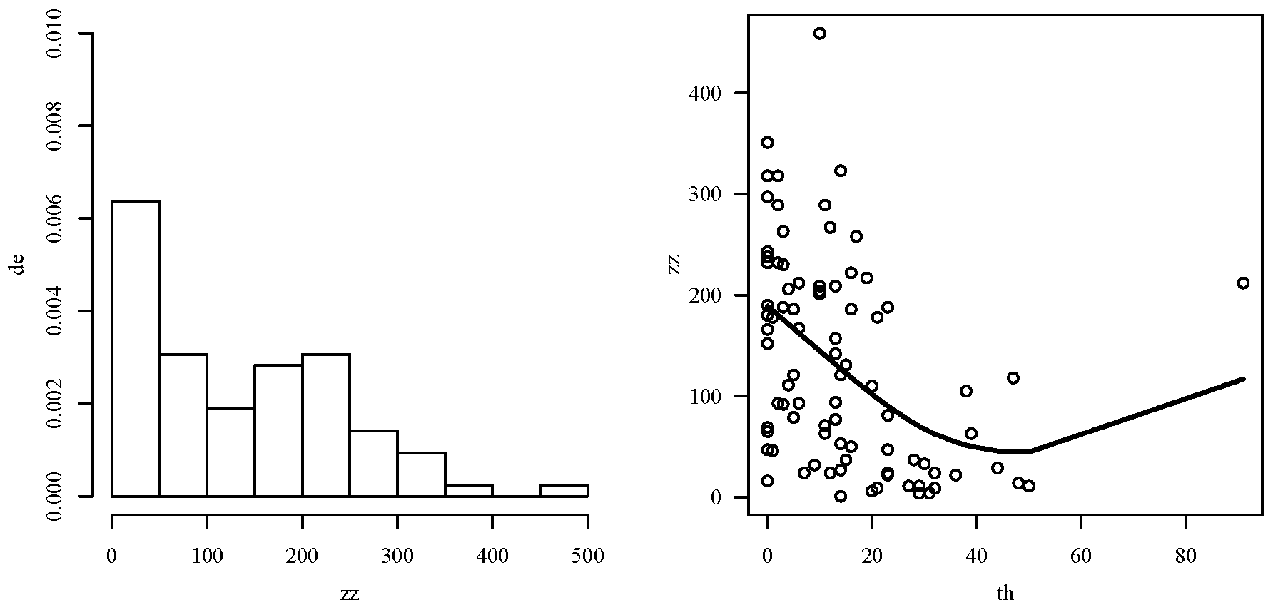
1.00	114.50	133.79	104.46	78.82	0.61	2.58	459.00	86

provides a descriptive summary of the observed vanadium concentration that includes median (MD), mean ($\overline{y}$), SD, CV, skewness (CS) and kurtosis (CK), and minimum ($y_{\left(1\right)}$) and maximum ($y_{\left(n\right)}$) values. The unit of measurement of the concentration (response variable) is parts-per million (ppm). From this table, note the positively skewed nature of the data distribution. The skewed nature is confirmed by the histogram of Figure 2 (left). In addition, Figure 2 (right) indicated some relationship between quantity of vanadium in terms of the quantity of thorium, which motivates the use of the REE regression model to study these variables.

5.2. Estimation and Model Checking

We consider the REE regression model with the structure: ${\eta }_i={\gamma }_0+{\gamma }_1{z}_{i1}$.

Table 5. ML estimates (with estimated asymptotic SEs in parentheses) for the RGA, RBS, and REE regression model for the fit mineral data set.

	Fitted Models
Parameter	RGA	RBS	REE
${\widehat{\gamma }}_0$	5.0734 (0.1252)	5.0271 (0.1767)	5.0440 (0.1122)
${\widehat{\gamma }}_1$	−0.0145 (0.0060)	−0.0172 (0.0063)	−0.0125 (0.0044)
p-value	[0.0148]	[0.0068]	[0.0049]
$\widehat{\varphi }$	1.1955 (0.1630)	-	-
$\widehat{\xi }$	-	0.8888 (0.1376)	-
$\widehat{\pi }$	-	-	0.4650 (0.1713)
log-likelihood	−503.3155	−520.3540	−502.5457
AIC	1012.6311	1046.7080	1011.0914
BIC	1019.9941	1054.0711	1018.4544

provides the estimation and hypothesis testing results for the REE regression model analyzing mineral data. Results of the RGA and RBS regression models are also detailed in this table, as well as their AIC (Akaike [24]), BIC (Schwarz [25]), and log-likelihood values.

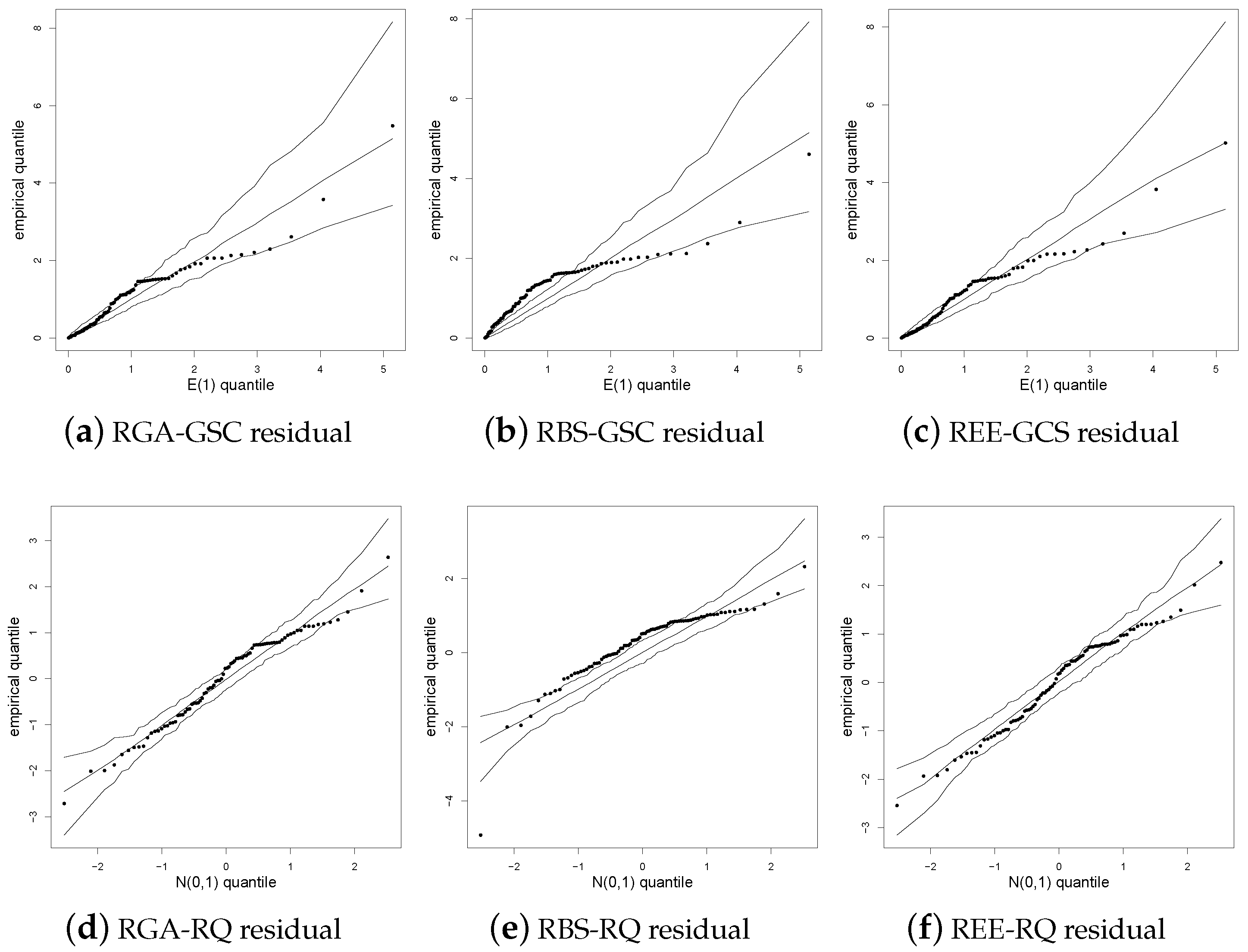
Figure 3 shows the QQ plots with simulated envelope for the GCS and QS residuals. These plots allow us to check graphically whether the GCS and QS residuals follow the EXP(1) and N(0, 1) distributions or not, respectively. From Figure 3, note that these residuals present a good agreement with their corresponding target distributions.

5.3. Diagnostic Analysis

Based on estimation and model validation results presented previously, we conducted a diagnostic analysis for the REE regression model, the suggested fitted model according to the analysis. Next, we carry out our diagnostic analysis based on global and local influence. First, Figure 4 presents the case-deletion measures GCD${}_i^c\left(\mathit{\psi }\right)$ and LD${}_i^c\left(\mathit{\psi }\right)$ discussed in Section 3.2. From this figure, LD${}_i^c\left(\mathit{\psi }\right)$ statistic indicates that the cases #25, #44, and #69 are potentially influential. On the other hand, the GCD${}_i^c\left(\mathit{\psi }\right)$ statistic does suggest case #44 as potentially influential.

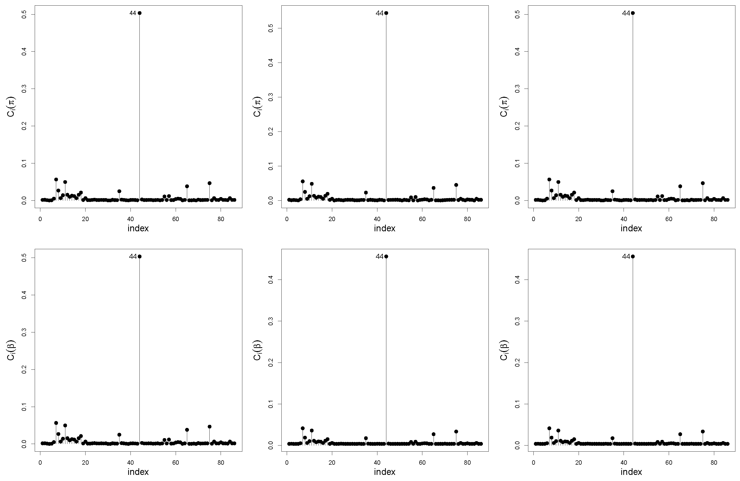
Index plots of $C_i$ for $\pi$ and $\mathit{\gamma }$ under the case-weight, response, and covariate perturbation schemes are displayed in Figure 5. Note that case #44 is detected as potentially influential on $\widehat{\pi }$ and $\widehat{\mathit{\gamma }}$ under the three perturbation schemes.

In order to check the impact on the model inference of the detected influential cases, we remove influential cases and reestimating the parameters as well as their corresponding SEs.

Table 6. ML estimates (with estimated asymptotic SEs in parentheses) for the RGA, RBS, and REE regression model for the fit mineral data set (without observation #44).

	Fitted Models
Parameter	RGA	RBS	REE
${\widehat{\gamma }}_0$	5.3248 (0.1240)	5.3260 (0.2020)	5.3008 (0.1276)
${\widehat{\gamma }}_1$	−0.0399 (0.0066)	−0.0453 (0.0101)	−0.0381 (0.0069)
p-value	[<0.0001]	[<0.0001]	[<0.0001]
$\widehat{\varphi }$	1.3865 (0.1925)	-	-
$\widehat{\xi }$	-	1.0595 (0.1640)	-
$\widehat{\pi }$	-	-	0.3056 (0.1548)
log-likelihood	−488.7114	−508.1733	−488.1657
AIC	983.4229	1022.3466	982.3314
BIC	990.7508	1029.6746	989.6594

shows the parameter estimates and their corresponding estimated SEs without observation #44. In addition, p-values are shown for the regression coefficients based on t-tests.

6. Conclusions

In the present paper, the reparameterization of the EE model based on the mean motivated us to propose a regression model for positive data. The maximum likelihood method is employed with the EM algorithm for estimating the model parameters. Application to real data with covariates was presented showed by the AIC and BIC criteria besides the deviance residuals in which the REE model fit better for this data set than the other reparameterizations considered.

The main contribution of this paper is to develop EM algorithms for maximum likelihood estimation as well as to apply Zhu and Lee’s approach for case-deletion measures and the local influence diagnostics in the linear regression models with REE errors. Closed-form expressions are obtained for the M and E steps of EM algorithm, for the observed information matrix, for the Hessian matrix $\ddot{\mathit{Q}}$, and for the $\Delta$matrix under three perturbation schemes. The models can be fitted using standard available software packages, like R (code available upon request).

References

- Fisher, R.A.; Tippett, L.H.C. Limiting forms of the frequency distribution of the largest and smallest member of a sample. Proc. Camb. Philos. Soc. 1928, 24, 180–190. [Google Scholar] [CrossRef]
- Gómez, Y.M.; Bolfarine, H.; Gómez, H.W. A New Extension of the Exponential Distribution. Colomb. J. Stat. 2014, 37, 25–34. [Google Scholar] [CrossRef] [Green Version]
- Ghitany, M.E.; Atieh, B.; Nadarajah, S. Lindley distribution and its application. Math. Comput. Simul. 2008, 78, 493–506. [Google Scholar] [CrossRef]
- Andrade, T.A.N.; Bourguignon, M.; Cordeiro, G.M. The exponentiated generalized extended exponential distribution. J. Data Sci. 2016, 14, 393–414. [Google Scholar]
- Rasekhi, M.; Alizadeh, M.; Altun, E.; Hamedani, G.G.; Afify, A.Z.; Ahmad, M. The Modified Exponential Distribution with Applications. Pak. J. Stat. 2017, 33, 383–398. [Google Scholar]
- Rasekhi, M.; Chatrabgoun, O.; Daneshkhah, A. Discrete Weighted Exponential Distribution: Properties and Applications. Filomat 2018, 32, 3043–3056. [Google Scholar] [CrossRef]
- Santos-Neto, M.; Cysneiros, F.J.; Leiva, V.; Barros, M. Reparameterized Birnbaum–Saunders regression models with varying precision. Electron. J. Stat. 2016, 10, 2825–2855. [Google Scholar] [CrossRef]
- Bourguignon, M.; Santos-Neto, M.; de Castro, M. A new regression model for positive data. arXiv 2018, arXiv:1804.07734. [Google Scholar]
- Bourguignon, M.; Leão, J.; Gallardo, D.I. Parametric modal regression with varying precision. Biom. J. 2020, 62, 2002–2020. [Google Scholar] [CrossRef]
- Dempster, A.P.; Laird, N.M.; Rubin, D.B. Maximum likelihood from incomplete data via the EM algorithm (with discussion). J. R. Stat. Soc. Ser. B 1977, 39, 1–38. [Google Scholar]
- Cook, R.D. Detection of influential observation in linear regression. Technometrics 1977, 19, 15–18. [Google Scholar]
- Cook, R.D. Assessment of local influence. J. R. Stat. Soc. Ser. B 1986, 48, 133–155. [Google Scholar] [CrossRef]
- Zhu, H.-T.; Lee, S.-Y. Local influence for incomplete data models. J. R. Stat. Soc. Ser. B 2001, 63, 111–126. [Google Scholar] [CrossRef]
- Bolboaca, S.D.; Jantschi, L. The Effect of Leverage and/or Influential on Structure-Activity Relationships. Comb. Chem. High Throughput Screen. 2013, 16, 288–297. [Google Scholar] [CrossRef]
- Jantschi, L. A Test Detecting the Outliers for Continuous Distributions Based on the Cumulative Distribution Function of the Data Being Tested. Symmetry 2019, 11, 835. [Google Scholar] [CrossRef] [Green Version]
- Lee, S.-Y.; Xu, L. Influence analyses of nonlinear mixed-effects models. Comput. Statist. Data Anal. 2004, 45, 321–341. [Google Scholar] [CrossRef]
- Dunn, P.K.; Smyth, G.K. Randomized quantile residuals. J. Comput. Graph. Stat. 1996, 5, 236–244. [Google Scholar]
- Cox, D.R.; Snell, E.J. A general definition of residuals. J. R. Stat. Soc. Ser. B 1968, 30, 248–265. [Google Scholar] [CrossRef]
- R Development Core Team. A Language and Environment for Statistical Computing; R Foundation for Statistical Computing: Vienna, Austria, 2019. [Google Scholar]
- Gómez, H.W.; Venegas, O.; Bolfarine, H. Skew-symmetric distributions generated by the distribution function of the normal distribution. Envirometrics 2006, 18, 395–407. [Google Scholar] [CrossRef] [Green Version]
- Bolfarine, H.; Gómez, H.W.; Rivas, L.I. The log-bimodal-skew-normal model. A geochemical application. J. Chemom. 2011, 25, 329–332. [Google Scholar] [CrossRef]
- Olmos, N.M.; Varela, H.; Gómez, H.W.; Bolfarine, H. An extension of the half-normal distribution. Stat. Pap. 2012, 53, 875–886. [Google Scholar] [CrossRef]
- Reyes, J.; Barranco-Chamorro, I.; Gallardo, D.I.; Gómez, H.W. Generalized Modified Slash Birnbaum–Saunders Distribution. Symmetry 2018, 10, 724. [Google Scholar] [CrossRef] [Green Version]
- Akaike, H. A new look at the statistical model identification. IEEE Trans. Autom. Control 1974, 19, 716–723. [Google Scholar] [CrossRef]
- Schwarz, G. Estimating the dimension of a model. Ann. Stat. 1978, 6, 461–464. [Google Scholar] [CrossRef]
Figure 1.
Plots of the REE PDF for indicated and (solid line), (dashed line), (dotted line) and (dotdash line).
Figure 2.
Histogram (left) and Scatterplot with smoothing curve (right) for mineral data.
Figure 3.
QQ plot with a simulated envelope under the indicated residual and model for mineral data.
Figure 4.
Likelihood displacement (left) and Generalized Cook (right) distance for mineral data.
Figure 5.
Index plots of for under the case-weight (left), response (center) and covariate (right) perturbation schemes with mineral data.