The Casimir Densities for a Sphere in the Milne Universe


1
Department of Physics, Yerevan State University, 1 Alex Manoogian Street, 0025 Yerevan, Armenia
2
Institute of Applied Problems in Physics NAS RA, 25 Nersessian Street, 0014 Yerevan, Armenia
*
Author to whom correspondence should be addressed.
†
These authors contributed equally to this work.
Symmetry 2020, 12(4), 619; https://doi.org/10.3390/sym12040619
Submission received: 17 March 2020
/
Revised: 28 March 2020
/
Accepted: 2 April 2020
/
Published: 14 April 2020
(This article belongs to the Special Issue Relativistic Gravity, Cosmology and Physics of Compact Stars)
Abstract
:The influence of a spherical boundary on the vacuum fluctuations of a massive scalar field is investigated in the background of a -dimensional Milne universe, assuming that the field obeys Robin boundary conditions on the sphere. The normalized mode functions are derived for the regions inside and outside the sphere and different vacuum states are discussed. For the conformal vacuum, the Hadamard function is decomposed into boundary-free and sphere-induced contributions and an integral representation is obtained for the latter in both the interior and exterior regions. As important local characteristics of the vacuum state, the vacuum expectation values (VEVs) of the field squared and of the energy-momentum tensor are investigated. It is shown that the vacuum energy-momentum tensor has an off-diagonal component that corresponds to the energy flux along the radial direction. Depending on the coefficient in Robin boundary conditions, the sphere-induced contribution to the vacuum energy and the energy flux can be either positive or negative. At late stages of the expansion and for a massive field the decay of the sphere-induced VEVs, as functions of time, is damping oscillatory. The geometry under consideration is conformally related to that for a static spacetime with negative constant curvature space and the sphere-induced contributions in the corresponding VEVs are compared.
1. Introduction
In constructing quantum field theories in background geometries different from the Minkowski spacetime, among the most important points is the selection of a physically meaningful vacuum state. The vacuum state depends on the choice of complete set of mode functions used in the second quantization procedure [1,2,3,4]. Those functions, and consequently the properties of the vacuum state, are sensitive to both the local and global characteristics of background spacetime. Already for the Minkowski bulk, depending on spacetime coordinates employed corresponding to different observers, different vacuum states are realized. An example is the Fulling–Rindler vacuum that presents the vacuum state for a uniformly accelerated observer different from the standard Minkowskian vacuum. The corresponding coordinates (Rindler coordinates) cover only a part of the Minkowski spacetime (R and L Rindler wedges). Other patches of the Minkowski spacetime inside the future and past light cones correspond to the so-called Milne universe. Quantum field theory in the Milne patches of the Minkowski spacetime has been discussed in [5,6,7,8,9,10,11,12,13] (see also [1,2,3,4]). The Milne universe is described by the Friedmann–Robertson–Walker type line element with negative curvature spatial sections and with the scale factor being a linear function of the time coordinate. It is well adapted for considerations of different types of the vacuum states in backgrounds with time-dependent metric tensors. Quantum fields in background of closely related geometries with linear scale factors and planar spatial sections have been considered in [14,15,16,17,18,19,20,21,22,23,24,25,26,27,28,29].
In the present paper we are interested in boundary-induced quantum effects in the Milne universe. The boundary conditions imposed on quantum fields modify the vacuum fluctuations and as a consequence of that the vacuum expectation values (VEVs) of physical observables are shifted compared to those for the geometry where the boundaries are absent. This is the well-known Casimir effect (for reviews see [30,31,32,33,34,35]). Explicit expressions for the vacuum characteristics can be obtained for highly symmetric bulk and boundary geometries. In particular, spherical boundaries have attracted a great deal of attention. The early investigations of the electromagnetic Casimir effect for a reflecting spherical boundary were motivated by the Casimir semiclassical model of an electron [36] where the Casimir pressure compensates outwardly-directed coulomb forces. However, the further studies of the Casimir effect for perfectly conducting spherical shell [37,38,39,40] have shown that the vacuum forces are outwardly-directed and, hence, cannot play the role of Poincaré stresses (for further investigations of the Casimir energy and forces in geometries with spherical boundaries see references in [30,31,32,33,34,35,41,42,43]).
More detailed information on the properties of the vacuum state is provided by local characteristics such as the VEVs of the field squared and of the energy-momentum tensor. The latter VEV also determines the back reaction of quantum effects on the background geometry and plays an important role in modeling of self-consistent dynamics on the base of semiclassical Einstein equations. The VEVs of the electric and magnetic field squared and of the energy density for electromagnetic and chromomagnetic vacuum fields within a spherical cavity with reflecting boundary have been studied in [44,45]. The VEVs for the remaining components of the energy-momentum tensor for the electromagnetic field inside and outside a spherical shell and in the region between two concentric spherical shells is investigated in [46,47,48,49] (these results are summarized in [50]). For a massive scalar field with the Robin boundary condition the VEVs of the energy-momentum tensor inside and outside a spherical shell and in the region between two concentric spherical boundaries in -dimensional Minkowski spacetime have been investigated in [51]. The corresponding VEVs in background of curved global monopole were discussed in [52,53,54,55,56] for scalar and spinor fields, respectively. The Casimir densities in the geometry of a global monopole with a general spherically symmetric static core of finite radius are investigated in [57,58]. The bulk and surface Casimir densities for spherical branes in Rindler-like spacetime , with a two-dimensional Rindler spacetime , have been studied in [59,60,61]. The latter geometry approximates the gravitational field near the horizon of -dimensional black holes. The VEV of the energy-momentum tensor for spherical boundaries on the background of dS spacetime is investigated in [62,63] for a conformally coupled massless scalar field and in [43] for a massive field with general curvature coupling parameter and with the Robin boundary condition. The scalar vacuum polarization and the expectation value of the energy-momentum tensor for spherical boundaries in the background of a constant negative curvature space are discussed in [64,65,66]. In [67] the two-point function and the VEVs are investigated for a scalar field in a spherically symmetric static background geometry with two distinct metric tensors inside and outside a spherical boundary. In this setup the exterior and interior geometries can correspond to different vacuum states of the same theory.
Here we investigate the local characteristics of the scalar vacuum inside and outside a spherical boundary in the Milne universe. The corresponding line element is conformally related to that for a static spacetime with constant negative curvature space with time-dependent conformal factor. Though the geometry of the Milne universe is flat, related to the time-dependence of the metric tensor, the Casimir problem for a spherical boundary in its background is more complicated than that discussed in [64,66] for a curved background.
The paper is organized as follows. In the next section we describe the bulk and boundary geometries and the structure of the modes for a scalar field with Robin boundary condition on a sphere. The mode functions are specified for the adiabatic and conformal vacua. In Section 3 the Hadamard function, the boundary-induced contributions in the VEVs of the field squared and of the energy-momentum tensor are investigated inside the spherical shell for the conformal vacuum. The behavior of the VEVs in asymptotic regions of the parameters are discussed and the results of the numerical analysis are presented. The similar investigation for the region outside the sphere is presented in Section 4. The main results of the paper are summarized in Section 5. In Appendix A we present a summation formula for series over the scalar eigenmodes inside the spherical shell that is used to derive an integral representation for the Hadamard function.
2. Geometry and the Scalar Field Modes
The -dimensional background spacetime we are going to consider is described by the line element
where , , and is the line element on a sphere with unit radius. The spatial part of the line element is written in terms of the hyperspherical coordinates with the set of angular coordinates , where . Note that the radial coordinate r is dimensionless. The line element (1) corresponds to the so-called Milne universe. The background spacetime is flat, however the spatial geometry corresponds to a negatively curved space.
The flatness of the geometry described by (1) is explicitly seen passing to new coordinates with
In terms of these coordinates the line element takes the standard Minkowskian form in spherical spatial coordinates:
From (2) we see that the coordinates cover the patch of the Minkowski spacetime inside the future light cone. In Figure 1 we have plotted the coordinate lines for in the Minkowskian half-plane . In the past light cone one has , , . The remaining region corresponds to the Rindler patch. From the cosmological point of view, the importance of the metric given by (1) is related to the fact that it is the late time attractor in a large class of Friedmann–Robertson–Walker open cosmological models.
Consider a massive scalar field with a curvature coupling parameter . The corresponding equation of motion reads
where is the covariant derivative operator and is the Ricci scalar for the background geometry. Though in the problem under consideration , the energy-momentum tensor depends on the curvature coupling parameter. We assume the presence of a spherical boundary with radius on which the scalar field obeys Robin boundary condition
where A and B are dimensionless constants, , with for the interior region and for the exterior region. Special cases and correspond to Dirichlet and Neumann boundary conditions. Let us denote by the radius of the sphere in terms of the Minkowskian radial coordinate R. From (2) we get . Hence, the boundary under consideration corresponds to a uniformly expanding sphere in the Minkowski spacetime with the velocity . We are interested in the influence of the sphere on the local properties of the vacuum state. Those properties are encoded in two-point functions and, as the first step, we shall evaluate these functions. In order to do that we need a complete set of mode functions for the field obeying the boundary condition (5).
In the hyperspherical coordinates the field equation is written as
where is the angular part of the Laplacian operator. In accordance with the problem symmetry, we present the solution in the form
where are the hyperspherical harmonics of degree l, where , , and are integers such that and
The hyperspherical harmonics obey the equation
and are normalized in accordance with
The explicit expression for is not required in the following discussion. One has the addition theorem
where the star menas the complex conjugate, is the angle between the directions determined by and , is the surface area of the sphere in D-dimensional space with unit radius, and is the Gegenbauer polynomial.
From here two separate equations are obtained:
where is the separation constant. Introducing a new radial function , we can see that the general solution for is a linear combination of the associated Legendre functions and (here the associated Legendre functions are defined in accordance with Ref. [68]) with the order and degree determined by
The relative coefficient in the linear combination depends on the spatial region under consideration and will be determined below.
The general solution for the function is presented in two equivalent forms
with constants and . The coefficients in two representations are related by
We will assume that the function is normalised by the condition
This leads to the following relations between the coefficients and :
For real z the corresponding relation between the coefficients and has the form
whereas for purely imaginary z we get
Hence, the mode functions for the scalar field are written as
where stands for the set of quantum numbers specifying the solutions, , and
with . By taking into account the condition (17) imposed on the function , from the normalization condition
we get the corresponding condition for the radial function:
where the integration goes inside or outside the sphere. After imposing the boundary condition, the normalized mode functions contain an arbitrary constant that should be fixed by the choice of the vacuum state.
In order to discuss the set of vacuum states it is convenient to introduce new coordinates according to
where a is a constant with dimension of length. In terms of these coordinates the line element is written in conformally static form
This shows that the background geometry under consideration is conformally related (with the conformal factor ) to the static spacetime with a constant negative curvature space. In the limit for fixed and , from (26) the Minkowskian line element in spherical coordinates is obtained. In this limit the quantum number appears in equations (13), written in terms of the coordinates , in the form of the ratio . The Minkowskian mode functions are obtained for fixed . This means that in the limit one has , with fixed w, and tends to infinity. The influence of a spherical boundary on the properties of the vacuum state for static spacetime with a negative constant curvature space (the corresponding line element is given by the expression in the square brackets of (26)) has been investigated in [64,66].
Let us consider the function (15) in the Minkowskian limit . Both the order and the argument of the cylindrical functions are large and we use the leading terms of the corresponding uniform asymptotic expansions. For the Hankel functions that gives
and , with and
By taking into account that to the leading order , we see that from the part in (15) with the Hankel function the Minkowskian positive energy mode functions are obtained. Hence, in order to obtain the Minkowskian vacuum one should take in (15) . This corresponds to the adiabatic vacuum, denoted here as (see also the discussion in [1,14]). For the corresponding function in (21) we have
In accordance with (26) for a conformally coupled massless scalar field the problem under consideration is conformally related to the corresponding problem in static spacetime with a constant negative curvature space. In the limit from (22) one has
where is the gamma function. For the case the mode functions (21) are conformally related to the corresponding positive energy mode functions in the static counterpart (with the energy ). From the relation (20) it follows that the quantum number z should be real for the modes realizing the corresponding vacuum. The latter is called as the conformal vacuum. The coefficient is found from (19) and the mode functions have the form (21) with
In what follows we will assume that the filed is prepared in the conformal vacuum. The mode function are different in the exterior and interior region of the sphere and we consider them separately.
3. Region inside the Sphere
3.1. Normalized Mode Functions
Inside the sphere, , for the modes (21) regular at the sphere center, in (22) one has . The mode functions realizing the conformal vacuum take the form
where is given by (30). As it has been explained in the previous section, in (31) . The corresponding eigenvalues are determined by the boundary condition (5). They are roots of the equation
For a given function , the barred notation in the right-hand side is defined in accordance with
with the coefficients
The corresponding positive solutions will be denoted by , . The set of quantum numbers are specified by .
The Equation (32) coincides with the eigenvalue equation inside a spherical boundary in static spacetime with a negative constant curvature space and the properties of the roots were discussed in [66]. It has been shown that for in addition to real roots the Equation (32) may have purely imaginary solutions. With given l and there are no purely imaginary zeros for sufficiently small values of . With increasing , started from some critical value , purely imaginary zeros , , appear. The critical value increases when l increases and the purely imaginary roots first appear for the lowest mode . For a given there are no purely imaginary zeros if . For the critical values of the Robin coefficient one has and they are decreasing function of . In Table 1, for the spatial dimension , we present the critical values of the Robin coefficient in the interior region for the mode and for different values of the sphere radius. As it has been discussed above, for the conformal vacuum the quantum number z should be real. Related to this, in what follows we will assume the values of for which all the roots of (32) are real.
For the integral in the normalization condition (24) is reduced to . By taking into account that are the roots of (32), the integral can be presented in the form
For the further consideration it is convenient to introduce the function
for . In the second representation we have used the relation
valid for . With the notation (36), the normalization constant is presented as
where is given by (14). Having specified the scalar modes, we turn to the evaluation of the Hadamard function inside the sphere.
3.2. Hadamard Function
The Hadamard function is defined as the VEV . Expanding the field operators in terms of the mode functions and using the commutation relations, it is presented in the form of the mode sum
With the mode functions from (31), for the Hadamard function one gets
where and we have introduced the notation
In (40), the summation over the roots of (32) is present. These roots are given implicitly and the representation (40) is not convenient for the investigation of the local characteristics of the vacuum state.
A representation more adapted for the further analysis is obtained by using the summation formula (A1) from Appendix A. For the series in (40) the corresponding function is given by
This function has simple poles at , . They correspond to the poles discussed in Appendix A. By taking into account the relation , we see that the function (42) is an even function. Hence, the term in (A1) containing the residues at the poles becomes zero. In the last integral of (A1) we use the relation [68]
Applying the summation formula (A1) with the function (42), the Hadamard function is presented as
where the part
is the corresponding function in the boundary-free geometry. The last term in (44) comes from the second integral in (A1) and is expressed as
where
and the integral is understood in the sense of the principal value.
For a massless field one has
with the conformal time from (25). In this case the sphere-induced contribution to the Hadamard function is transformed to
where
is the Hadamard function for a conformally coupled massless field in a static spacetime with a negative constant curvature space (see [66]). The line element for the latter geometry is given by the expression in the square brackets of (26) and :
3.3. VEV of the Field Squared
The VEV of the field squared is obtained from the Hadamard function in the coincidence limit of the arguments. That limit is divergent and a renormalization is required. For points away from the sphere the divergences are contained in the boundary-free part only. The VEV is decomposed as
where is the renormalized VEV in the boundary-free geometry for the conformal vacuum and the sphere-induced contribution is given by
Here
is the degeneracy of the angular mode with given l and we have introduced the function
Note that in the absence of the spherical boundary the geometry under consideration is homogeneous and the renormalized boundary-free VEV will depend on the time coordinate only.
For a massless field one has
and the function (55) does not depend on the time coordinate. In this case we get
where
is the VEV for a massless conformally coupled field in a static negative constant curvature space.
For a massive field and in the limit to the leading order one finds
For large values of t, , we use the asymptotic expression
The leading term in the boundary-induced VEV is presented as
As seen, for a massive field the late-time asymptotic of contains two parts. The first one is monotonically decreasing as and the behavior of the second one is damping oscillatory, as . For a massless field the decay is monotonic, like .
The VEV (53) diverges on the boundary . For points near the sphere the dominant contribution comes from large values of l and x. By taking into account that for large x one has , we see that the leading term in the asymptotic expansion near the sphere is obtained from that for (58) by the replacement :
Note that is the proper distance from the sphere and the leading term (62) coincides with that for a sphere in the Minkowski bulk with the distance from the sphere replaced by the proper distance in the geometry under consideration. As seen from (62), near the sphere the boundary-induced contribution in the VEV of the field squared is negative for Dirichlet boundary condition and positive for non-Dirichlet boundary conditions. By taking into account that for small r one has
we can see that at the sphere center the only nonzero contribution comes from the mode with and we get
For this expression is further simplified to
where .
The integral in (53) is understood in the sense of the principal value. For numerical calculations it is convenient to present it in an alternative form, where the integrand has no poles. Let us consider the integral of the form , understood in the sense of the principal value. By using the formula (prime on the summation sign means that the term should be taken with coefficient 1/2)
and the fact that the principal value of the integral is zero, the integral is presented as
In this form the integrand is regular at the points .
In the left panel of Figure 2, for the Milne universe with , we have plotted the sphere-induced contribution in the VEV of the field squared inside a spherical shell versus the radial coordinate r for the values of the sphere radius (numbers near the curves) and for . The right panel presents the time-dependence of the same quantity for fixed r (numbers near the curves) and for . The VEV for the exterior region is displayed as well (). The corresponding analysis will be given in Section 4 below. On both the panels in Figure 2 the full curves correspond to Dirichlet boundary condition and the dashed curves correspond to Robin boundary condition with . Near the sphere the asymptotics are given by (62) and the boundary-induced VEV, as a function of the radial coordinate, behaves as . For we have the conformal relation (59) and the VEV behaves as . In that region the boundary-induced VEV in the field squared is a monotonic function of . That is not the case for . As it has been shown before by the asymptotic analysis (see (61)), for the VEV exhibits oscillatory damping behaviour and it can be either positive or negative. That behavior is also confirmed by numerical analysis. For example, in the case of Dirichlet boundary condition and for , (the case corresponding to the right panel of Figure 2) with increasing the VEV becomes zero at and then takes the local maximum at . After that again becomes zero at with the further damping oscillatory behavior as a function of .
Figure 3 displays the dependence of the sphere-induced VEV on the coefficient in Robin boundary condition for , , . The numbers near the curves correspond to the values of the radial coordinate r. For the interior region we have taken . As seen, depending on the values of the Robin coefficient, the boundary-induced VEV changes the sign. It becomes zero at . For ( corresponds to Dirichlet boundary condition) the VEV is negative and it becomes positive with increasing . For the interior region (the graph for ), the VEV increases when approaches the critical value (see Table 1). For close to that critical value the dominant contribution to the VEV (53) comes from the mode . In the range the VEV is negative at . By taking into account that near the sphere it is positive, we conclude that for values of in that range the VEV , considered as a function of r, changes the sign.
In the evaluation of the VEV of the energy-momentum tensor the covariant d’Alembertian of the VEV of the field squared is required. The sphere-induced contribution in the latter is presented in the form
Note that for the radial part of the function we have the equation
This equation can be used to exclude the second derivative from the expressions of the VEV for the energy-momentum tensor.
3.4. VEV of the Energy-Momentum Tensor
Another important local characteristic for the vacuum state is the VEV of the energy-momentum tensor. Having the Hadamard function and the VEV of the field squared, that VEV is evaluated by using the formula
where for the geometry at hand the Ricci tensor vanishes, , and for the d’Alembertian acted on the VEV of the field squared one has (68). In (70) we have used the expression for the classical energy-momentum tensor that differs from the standard one (given, for example, in [1]) by the term that vanishes on the solutions of the field equation (see [69]). The VEV of the energy-momentum tensor is decomposed as
with the boundary-free and the sphere-induced contributions and , respectively. Similar to the case of the field squared, the renormalized boundary-free contribution will depend on the time coordinate only. It is diagonal and the corresponding vacuum stresses are isotropic . The background geometry is flat and for a conformally coupled massless field the vacuum energy-momentum tensor is traceless, (the conformal anomaly is absent). In this case .
The diagonal components of the sphere-induced VEV of the energy-momentum tensor are presented in the form (no summation over k)
where the operators for separate components are given by the expressions
and for . In (73), is the curvature coupling parameter for a conformally coupled scalar field. The boundary-induced VEVs (72) obey the trace relation
For a conformally coupled massless field the boundary-induced VEV of the energy-momentum tensor is traceless. The background geometry is flat and the latter is the case for the boundary-free part as well.
The problem under consideration is inhomogeneous with respect to the coordinates t and r. As a consequence of that the VEV of the energy-momentum tensor has nonzero off-diagonal component
This component describes energy flux along the radial direction. The boundary-free part in vanishes and (75) is induced by the sphere. For a massless field the function does not depend on time and in the case of conformal coupling () the energy flux vanishes. Of course, we could expect this result on the base of the conformal relation of the problem at hand to the corresponding problem in static spacetime with negative constant curvature space.
The sphere-induced VEVs obey the covariant conservation equation for the energy-momentum tensor, with . The latter is reduced to the following two relations
The component determines the contribution of the spherical boundary to the vacuum energy density. The boundary-induced part of the vacuum energy in the spatial volume V with a boundary is given by (in the coordinates with )
where g is the determinant of the metric tensor. From the equation (the first equation in (76)) we get
where the Greek indices run over . In (78), , , is the external normal to the boundary and h is the determinant of the induced spatial metric on . From (78) we see that the energy flux density per unit proper surface area is given by . Note that for a spherical boundary of radius r with the center at one has , where the upper/lower sign corresponds to the volume V inside/outside the sphere. The energy flux is directed from the sphere if and towards the sphere if . From here it follows that for the interior region the energy flux is directed from the sphere for and towards the sphere for .
For a massless field the function is given by (56) and does not depend on t. In this case the terms in the expressions (73) for the operators containing derivatives over t can be removed. For a conformally coupled massless field one gets
and the off-diagonal component of the vacuum energy-momentum tensor vanishes. Now we have the conformal relation (no summation over k) , where the VEV in static spacetime with constant negative curvature space is given by
with from (79). It can be checked that (80) coincides with the result from [66] for a conformally coupled massless field.
The general expressions for the VEVs of the components of the energy-momentum tensor are rather complicated and we turn to the investigation of their behavior in the asymptotic regions of the parameters. In the limit (early stages of the expansion) one has and to the leading order for the diagonal components we get , where is the corresponding VEV for a massless field with curvature coupling parameter in static spacetime with a negative constant curvature space. For the energy flux and for non-conformally coupled fields () we have
The leading term in the right-hand side does not depend on the field mass. In the case of massless fields the relation (81) is exact. For a conformally coupled field we need to keep the next to the leading order terms in the expansion of the product . This leads to the result
for . Here the integrand has a simple pole at and the integral is understood in the sense of the principal value.
Now let us consider the late stages of the expansion, . By using the corresponding asymptotic expression (60), we see that the dominant contributions come from the term with in (60) and from the parts in (73) with . The leading term in the VEV of the energy density vanishes. To the leading order, the vacuum stresses are isotropic and (no summation over )
For the energy flux from (75) we get
The leading term in the energy density can be found from the first relation in (76):
with from (83). Note that the dependence on the curvature coupling parameter enters in the form of the coefficient . In particular, the leading term in the asymptotic for a minimally coupled field is obtained from that for a conformally coupled field multiplying by D. As seen from the asymptotic expressions (83)–(85), at late stages of the expansion the behavior of the sphere-induced contributions in the VEVs, as functions of the time coordinate, is oscillatory damping.
By using (63), we see that at the sphere center the nonzero contributions come from the terms . The energy flux vanishes at the sphere center and for small r it is given by
Similar to the field squared, the VEV of the energy-momentum tensor is divergent on the sphere. The leading terms in the energy density and tangential stresses are found from (72) by using the asymptotic . They are given by (no summation over )
The leading term in the radial stress vanishes. In order to find the corresponding asymptotic we first consider the leading term for the energy flux. The latter is found from the first equation of (76):
Note that the leading term (87) in the energy density and the tangential stresses coincides with that for spherical boundary in the Minkowski bulk where the distance from the sphere is replaced by the proper distance for the geometry (1). For a conformally coupled field the leading terms in the asymptotic expansion over the distance from the boundary vanish and the divergences on the sphere are weaker. As seen from (87), for a minimally coupled field the energy density near the sphere is negative for Dirichlet boundary condition and positive for non-Dirichlet conditions. Combining this with (88) we see that for a minimally coupled field and near the sphere the energy flux in the interior region is directed from the sphere for Dirichlet boundary condition and towards the sphere for non-Dirichlet boundary conditions.
In Figure 4, for the Milne universe and for a minimally coupled field, the boundary-induced VEV in the energy density is displayed as a function of the radial (left panel) and time (right panel) coordinates. The full and dashed curves correspond to Dirichlet and Robin boundary conditions. For the latter we have taken . For the left panel and the numbers near the curves correspond to the values of the sphere radius. The graphs on the right panel are plotted for and the numbers near the curves are the values of the radial coordinate r. Near the sphere the energy density behaves as . It is negative for Dirichlet boundary condition and positive for non-Dirichlet conditions. For an example presented in the left panel of Figure 4 in the case of Robin boundary condition the energy density is positive for all values of the radial coordinate inside the sphere. That is not the case for general values of . Depending on the latter, the energy density may change the sign. Considered as a function of the time coordinate, in the initial stages of the expansion the sphere-induced energy density behaves like . At late stages, , it decays as . Recall that for a massless field the late-time decay is monotonic, as .
The same graphs as in Figure 4 are plotted for a conformally coupled scalar field in Figure 5. In this case the divergence of the boundary induced VEV on the sphere is weaker. At late stages, corresponding to , the leading term in the asymptotic expansion of for a conformally coupled field differs from that for a minimally coupled field by an additional coefficient (with for the example in Figure 5).
Figure 6 presents the dependence of the sphere-induced VEV in the energy density on the coefficient in the Robin boundary condition for minimally (left panel) and conformally (right panel) coupled scalar fields. The graphs are plotted for , and the numbers near the curves are the values of the coordinate r. For the interior region we have taken and the corresponding VEV becomes zero at for a minimally coupled field and at for a conformally coupled field. For smaller values of the energy density is negative. By taking into account that for a minimally coupled field the corresponding energy density is positive near the sphere we see that it changes the sign as a function of the radial coordinate for sufficiently small values of .
Having discussed the behavior of the sphere-induced contribution to the VEV of the energy density, we turn to the investigation of the VEV for the energy flux. As it has been mentioned above, the energy flux density per unit proper surface area is given by . Figure 7 presents the energy flux density for a spherical boundary in the Milne universe and for a minimally coupled scalar field versus the radial (left panel) and time (right panel) coordinates. The values of the parameters are the same as those for Figure 4. As it has been already shown before by the asymptotic analysis, the energy flux linearly vanishes at the sphere center. For the values of the parameters corresponding to the left panel of Figure 7 the energy flux is directed from the sphere for Dirichlet boundary condition and towards the sphere for Robin boundary condition. For the leading term in the asymptotic expansion is given by (81) and the energy flux behaves like (the right panel in Figure 7). At late stages of the expansion, , the energy flux exhibits oscillatory damping behavior, . The same graphs for a conformally coupled field are displayed in Figure 8. The qualitative behavior of the energy flux is similar to that for the case of a minimally coupled field. Now, the divergence on the sphere is weaker and the corresponding VEV is smaller by the modulus.
The dependence of the energy flux density on the coefficient in the Robin boundary condition is depicted in Figure 9 for the same values of the parameters as in Figure 6. As seen from the graphs, in both the cases of minimally and conformally coupled fields, depending on the value of the Robin coefficient, the energy flux can be either positive or negative.
4. Exterior Region
4.1. Scalar Modes and the Hadamard Function
In this section we consider the VEVs in the region outside the sphere, . As a general solution of the radial equation we take the linear combination of the associated Legendre functions and . One of the coefficients is determined by the boundary condition (5) and the second one is found from the normalization condition. The mode functions realizing the conformal vacuum are presented as
where the function is given by (30), is a normalization constant and
The normalization coefficient is determined from the condition (24) with . For the region outside the sphere it takes the form
For the evaluation of the integral we note that it diverges for and the dominant contribution comes from large values of u. By using the corresponding asymptotic expressions for the functions and we can show that
On the base of this, from (92) for the normalization coefficient one finds
Note that for a spherical boundary in the static spacetime with a constant negative curvature space (the corresponding line element is given by (51)) in addition to the modes with real z one may have the modes with purely imaginary z, . For those modes the radial part of the mode functions is given by . The allowed values for are determined by the boundary condition on the sphere and they are roots of the equation . As it has been discussed in [66], for a given l the latter equation has no solution for with some critical value . The latter obeys the conditions , , and . As it has been discussed above, in the problem at hand with the line element (1) and for the conformal vacuum the quantum number z should be real. In what follows we will assume the values of the Robin coefficient in the region , where the equation has no solution.
Substituting the mode functions into the mode sum formula (39) with replaced by the integral , for the Hadamard function in the region we get the representation
where stands for the complex conjugate of the first term in the figure braces. In order to extract the part in (95) induced by the spherical boundary, we subtract the Hadamard function for the boundary-free geometry, given by (45).
The sphere-induced contribution to the Hadamard function, , can be further transformed by using the relation
As the next step, in the integral involving the right-hand side of (96) we rotate the contour of integration by the angle for the term with and by the angle for the term with . The poles , , are avoided by small semicircles in the right half-plane with radii . In the limit the contributions of the integrals over the semicircles in the upper and lower half-planes cancel each other and the integral is reduced to the principal value of the integral over the positive imaginary semiaxis. The product of the associated Legendre functions is transformed to . By using the relation
for the boundary-induced contribution in the Hadamard function we find the final representation
Note that we consider the values of the Robin coefficient for which the function in the integrand has no zeros. Comparing (98) with (46), we see that the expressions for the boundary-induced Hadamard functions inside and outside the sphere differ by the interchange
of the associated Legendre functions. Similar to (46), the integral in (98) is understood in the sense of the principal value.
The Hadamard functions in the interior and exterior regions, given above, characterize the correlations of vacuum fluctuations at different spacetime points. Another important global characteristic of the quantum fluctuations correlations is the entanglement entropy. For a scalar field in two regions of de Sitter spacetime separated by a spherical boundary, the entanglement entropy has been investigated in [70,71,72,73,74]. Note that in those references the de Sitter hyperbolic open charts were used with the spatial sections similar to (1). The corresponding mode functions for scalar fields with general curvature coupling parameter have been discussed in [75]. Similar investigations for the entanglement entropy can be done in the Milne Universe for the conformal vacuum by using the mode functions presented above.
4.2. VEVs of the Field Squared and Energy-Momentum Tensor
Taking the coincidence limit in (98) we find the sphere-induced part in the VEV of the field squared outside the sphere:
where
For a massless field the result (100) is conformally related to the corresponding expression for a conformally coupled massless scalar field in static spacetime with a negative constant curvature space (see (57)). In the exterior region the VEV has the form (58) with the replacements (99). In the early stages of the expansion, , the leading term is given by (59) and the boundary-induced VEV behaves as . At late stages of the expansion the asymptotic behavior of is described by (61) with the replacements (99).
Near the sphere the leading term in the asymptotic expansion of the sphere-induced VEV in the field squared is given by (62) with the replacement . At large distances from the sphere, assuming that for fixed , we can use the asymptotic expression
The dominant contribution to the integral in (100) comes from the region near the lower limit and to the leading order we get
The VEV is exponentially suppressed for both massive and massless fields. Note that for a spherical boundary in the static geometry described by (51), at large distances from the sphere the boundary-induced contribution behaves like (see [66]) , with . It is assumed that the expression under the square root is nonnegative (for negative values the vacuum state is unstable). For the decay of the sphere-induced VEV in the static spacetime is stronger.
In Figure 10 we have displayed the sphere induced contribution in the VEV of the field squared outside the spherical shell as a function of the radial coordinate. The graphs are plotted for , , and for the sphere radius (the numbers near the curves). The full curves correspond to Dirichlet boundary condition and the dashed curves present the case of Robin boundary condition with . Examples of the dependence of on time and on the Robin coefficient are presented in Figure 2 (right panel) and Figure 3. Note that for the Robin coefficient in the exterior region we have taken the values for which the function in the integrand of (100) has no zeros.
The VEV of the energy-momentum tensor is found on the base of (98) and (100) by using the formula (70). The calculations are similar to that for the interior region and for the diagonal components we get (no summation over k)
with the operators from (73). The expression for the VEV of the off-diagonal component reads
The VEVs are connected by the trace relation (74) and by the covariant continuity equations (76). For a massless field one has
and the expressions for the operators are simplified omitting the terms with time derivatives. In this special case for the energy flux one gets
It vanishes for a conformally coupled field. In the latter case the VEVs of the diagonal components are obtained from those for a spherical boundary in a static spacetime with negative constant curvature space by conformal transformation, , where is given by (80) with the replacements (99).
Now let us consider the asymptotics at early and late stages of the expansion. For , in the leading order the function does not depend on time and for the diagonal components we find , where is the VEV in static spacetime for a massless field with curvature coupling parameter . In the case of a non-conformally coupled field the leading term in the energy flux is given by the right-hand side of (107). In order to find the asymptotic of the energy flux for a conformally coupled field one needs the next to the leading term in the expansion of the function . In this case the leading term in the expansion of the energy flux at early stages is given by the right-hand side of (82) with the replacements (99). At late stages of the expansion, , the corresponding asymptotics are given by (83)–(85), again, with replacements (99).
Similar to the interior region, the VEVs (104) diverge on the sphere. The leading terms in the expansions of the energy density and of the tangential stresses over the distance from the sphere are given by (87) with the replacement . Hence, near the sphere these components have the same sign for the interior and exterior regions. The relations (88) and (89) between the energy flux, normal stress and energy density near the sphere remain the same in the exterior region. Consequently, near the sphere the components and have opposite signs in the exterior and interior regions. At large distances from the sphere we use the asymptotic expression (102). The main contribution to the sphere-induced VEVs comes from the region of the integration near the lower limit. For the diagonal components to the leading order we find (no summation over k)
where
and . In a similar way, for the energy flux one gets
Note that for a sphere in static spacetime with constant negative curvature space and for , at large distances the boundary-induced VEVs in the diagonal components decay as . For the sphere-induced VEVs in the static problem behave like (no summation over k) .
The Figure 11 and Figure 12 present the radial dependence of the sphere-induced contributions in the energy density and in the energy flux density for , and for several values of the sphere radius (numbers near the curves). The left and right panels correspond to minimally and conformally coupled fields, respectively. Similar to the interior region, for the values of the parameters corresponding to Figure 12 the energy flux is directed from the sphere for Dirichlet boundary condition and towards the sphere for Robin boundary condition.
5. Conclusions
We have investigated the influence of a spherical boundary on the local properties of the vacuum state for a scalar field in the Milne universe. The corresponding spacetime metric is flat with spatial sections having a constant negative curvature and the scale factor is a linear function of time. In the Minkowskian coordinates, the boundary under consideration corresponds to a uniformly expanding spherical shell. The mode functions are found in general case and they are specified for special cases of the adiabatic and conformal vacua. Further consideration for the two-point functions and for the VEVs is presented in the case of the conformal vacuum. Inside the sphere the eigenvalues of the quantum number z are solutions of the Equation (32) with the barred notation from (33). Depending on the value of the coefficient in Robin boundary condition, that equation may have purely imaginary roots. By taking into account that for the conformal vacuum z should be real, we specify the corresponding region for the values of . In the model under consideration all the information on the properties of the vacuum state is encoded in two-point functions. As such we have considered the Hadamard function. The corresponding mode sum for the interior region contains series over the roots of the eigenvalue Equation (32). For the summation of the series, a variant of the generalized Abel–Plana formula is used. As a result of that the contribution of the sphere is explicitly extracted. Among the advantages of the corresponding integral representation is that the explicit knowledge of the eigenvalues for the quantum number z is not required.
Then, on the base of the Hadamard function, we have investigated the VEVs of the field squared and of the energy-momentum tensor inside the sphere. They are decomposed into the boundary-free and sphere-induced contributions. The geometry under consideration is conformally related to the problem with a spherical boundary in a static spacetime with a constant negative curvature space and it is explicitly checked that for a conformally coupled massless scalar field the corresponding VEVs are connected by standard conformal relations. In that special case the energy flux vanishes. For non-conformally coupled or for massive fields, a new qualitative feature, induced by the sphere, is the appearance of the nonzero off-diagonal component of the vacuum energy-momentum tensor that describes energy flux along the radial direction. Depending on the values of the parameters, the flux can be directed either from the sphere or towards the sphere. For a massless field the time dependence is of the form for the VEV of the field squared and of the form for the diagonal components of the energy-momentum tensor and for the energy flux .
The general formulas for the VEVs are rather complicated and, in order to clarify their behavior, we have considered various asymptotic regions of the parameters. Near the sphere the boundary-induced contributions dominate in the total VEVs and the leading terms in the corresponding asymptotic expansions for the VEV of the field squared, for the energy density and for tangential stresses are the same as those for a sphere in the Minkowski spacetime (with the distance from the sphere replaced by the proper distance in the Milne universe). For the normal stress and energy flux the divergence on the sphere is weaker and the leading terms are given by (88) and (89). At early stages of the expansion, , the leading terms in the corresponding asymptotics for the VEVs of the field squared and of the diagonal components of the energy-momentum tensor are conformally related to the VEVs in static spacetime with a constant negative curvature space. The VEV of the field squared behaves as and the diagonal components behave like . The asymptotic of the energy flux at early stages is given by (81). At late stages of the expansion and for massive fields, assuming that , the VEVs exhibit damping oscillatory behavior. The corresponding asymptotics are given by (61) for the field squared and by (83)–(85) for the energy-momentum tensor. All these features are displayed by numerical examples. In particular, we have demonstrated that, depending on the Robin coefficient, both the sphere-induced energy density and the energy flux can be either positive or negative.
In the region outside the sphere the eigenvalues of the quantum number z are continuous and the mode functions are given by (90). The integral representations for the sphere-induced contributions to the Hadamard function and to the VEVs of the field squared and energy-momentum tensor differ from the corresponding expressions for the interior region by the replacement (99) of the associated Legendre functions. For the corresponding formulas the range of the allowed values for the Robin coefficient is wider compared to that for the interior region. Near the sphere and for non-conformally coupled fields the VEVs of the field squared, of the energy density and of the tangential stresses have the same sign in the exterior and interior regions. The VEVs of the normal stress and of the off-diagonal component have opposite signs. At large distances from the sphere the boundary-induced VEVs decay exponentially, like for both massive and massless fields. For massive conformally and minimally coupled fields and for a spherical boundary in a static spacetime with constant negative curvature space the decay at large distances is stronger.
Author Contributions
Investigation, A.A.S. and T.A.P.; software, T.A.P.; writing—original draft preparation, A.A.S. and T.A.P.; writing—review and editing, A.A.S. All authors have read and agreed to the published version of the manuscript.
Funding
This research received no external funding.
Conflicts of Interest
The authors declare no conflict of interest.
Appendix A. Summation Formula
The VEVs of physical observables inside a spherical shell in the Milne universe are expressed in terms of the series of the type , where is the kth positive root of the Equation (32). A summation formula for those series with a function analytic in the right-half plane , has been derived in [66] (see also [64] for the case ). Additional conditions imposed on the function were formulated in [66]. In particular, it was assumed that the function has no poles on the imaginary axis. In the physical problem we consider in the present paper the corresponding function has simple poles , , at the zeros of the function in (41). The generalization of the summation formula from [66] for the case of functions having simple poles on the imaginary axis is straightforward.
If the function is real for real x, then one has . From here it follows that if is a pole of the function then is also a pole. Hence, the poles on the imaginary axis are of the form , . The procedure to obtain the summation formula from the generalized Abel–Plana formula is similar to that used in [66]. The difference is that now the poles should be avoided by small semicircles with radii in the right half-plane and with the centers at the points . In the limit the contributions of the integrals over those contours are expressed in terms of the corresponding residues and the integral over the imaginary axis should be understood in the sense of the principal value. The summation formula takes the form
The remaining conditions on the function are the same as in [66]. Namely, it is assumed that for it obeys the condition for , where and for .
References
- Birrell, N.D.; Davies, P.C.W. Quantum Fields in Curved Space; Cambridge University Press: Cambridge, UK, 1982. [Google Scholar]
- Grib, A.A.; Mamayev, S.G.; Mostepanenko, V.M. Vacuum Quantum Effects in Strong Fields; Friedmann Laboratory Publishing: St. Petersburg, Russia, 1994. [Google Scholar]
- Fulling, S.A. Aspects of Quantum Field Theory in Curved Space-Time; Cambridge University Press: Cambridge, UK, 1996. [Google Scholar]
- Parker, L.; Toms, D. Quantum Field Theory in Curved Spacetime: Quantized Fields and Gravity; Cambridge University Press: Cambridge, UK, 2009. [Google Scholar]
- Sommerfield, C.M. Quantization on spacetime hyperboloids. Ann. Phys. 1974, 84, 285–302. [Google Scholar] [CrossRef]
- Gromes, D.; Rothe, H.; Stech, B. Field quantization on the surface X2 = constant. Nucl. Phys. B 1974, 75, 313–332. [Google Scholar] [CrossRef]
- DiSessa, A. Quantization on hyperboloids and full space-time field expansion. J. Math. Phys. 1974, 15, 1892–1900. [Google Scholar] [CrossRef]
- Davies, P.C.W.; Fulling, S.A. Quantum vacuum energy in two dimensional space-times. Proc. R. Soc. Lond. A 1977, 354, 59–77. [Google Scholar]
- Bunch, T.S. Stress tensor of massless conformal quantum fields in hyperbolic universes. Phys. Rev. D 1978, 18, 1844. [Google Scholar] [CrossRef]
- Bunch, T.S.; Christensen, S.M.; Fulling, S.A. Massive quantum field theory in two-dimensional Robertson-Walker space-time. Phys. Rev. D 1978, 18, 4435. [Google Scholar] [CrossRef]
- Yamamoto, K.; Tanaka, T.; Sasaki, M. Particle spectrum created through bubble nucleation and quantum field theory in the Milne universe. Phys. Rev. D 1995, 51, 2968. [Google Scholar] [CrossRef] [Green Version]
- Tanaka, T.; Sasaki, M. Quantized gravitational waves in the Milne universe. Phys. Rev. D 1997, 55, 6061. [Google Scholar] [CrossRef] [Green Version]
- Higuchi, A.; Iso, S.; Ueda, K.; Yamamoto, K. Entanglement of the vacuum between left, right, future, and past: The origin of entanglement-induced quantum radiation. Phys. Rev. D 2017, 96, 083531. [Google Scholar] [CrossRef] [Green Version]
- Fulling, S.A.; Parker, L.; Hu, B.L. Conformal energy-momentum tensor in curved spacetime: Adiabatic regularization and renormalization. Phys. Rev. D 1974, 10, 3905. [Google Scholar] [CrossRef]
- Chitre, D.M.; Hartle, J.B. Path-integral quantization and cosmological particle production: An example. Phys. Rev. D 1977, 16, 251. [Google Scholar] [CrossRef]
- Nariai, H. On a quantized scalar field in some Bianchi-type I universe. Prog. Theor. Phys. 1977, 58, 560–574. [Google Scholar] [CrossRef] [Green Version]
- Nariai, H. On a quantized scalar field in some Bianchi-type I universe. II: DeWitt’s two vacuum states connected causally. Prog. Theor. Phys. 1977, 58, 842–849. [Google Scholar] [CrossRef] [Green Version]
- Nariai, H.; Tomimatsu, A. On the creation of scalar particles in an isotropic universe. Prog. Theor. Phys. 1978, 59, 296–298. [Google Scholar] [CrossRef] [Green Version]
- Nariai, H. Canonical approach to the creation of scalar particles in the Chitre-Hartle model-universe. Prog. Theor. Phys. 1980, 63, 324–326. [Google Scholar] [CrossRef] [Green Version]
- Mensky, M.B.; Karmanov, O.Y. Application of the propagator method to pair production in the Robertson-Walker metric. Gen. Rel. Grav. 1980, 12, 267–277. [Google Scholar] [CrossRef]
- Azuma, T. The renormalized energy-momentum tensor in a Robertson-Walker universe. Prog. Theor. Phys. 1981, 66, 892–902. [Google Scholar] [CrossRef] [Green Version]
- Charach, C.; Parker, L. Uniqueness of the propagator in spacetime with cosmological singularity. Phys. Rev. D 1981, 24, 3023. [Google Scholar] [CrossRef]
- Charach, C. Feynman propagators and particle creation in linearly expanding Bianchi type-I universes. Phys. Rev. D 1982, 26, 3367. [Google Scholar] [CrossRef]
- Azuma, T.; Tomimatsu, A. Low-energy behavior of a quantized scalar field in the linearly expanding universe. Gen. Rel. Grav. 1982, 14, 629–636. [Google Scholar] [CrossRef]
- Calzetta, E.; Castagnino, M. Feynman propagator in a linearly expanding universe. Phys. Rev. D 1983, 28, 1298. [Google Scholar] [CrossRef]
- Buchbinder, I.L.; Kirillova, E.N.; Odintsov, S.D. The Green functions in curved spacetime. Class. Quantum Grav. 1987, 4, 711. [Google Scholar] [CrossRef]
- Winters-Hilt, S.; Redmount, I.H.; Parker, L. Physical distinction among alternative vacuum states in flat spacetime geometries. Phys. Rev. D 1999, 60, 124017. [Google Scholar] [CrossRef]
- Tolley, A.J.; Turok, N. Quantum fields in a big-crunch-big-bang spacetime. Phys. Rev. D 2002, 66, 106005. [Google Scholar] [CrossRef] [Green Version]
- Saharian, A.A.; Petrosyan, T.A.; Abajyan, S.V.; Nersisyan, B.B. Scalar Casimir effect in a linearly expanding universe. Int. J. Geom. Methods Mod. Phys. 2018, 15, 1850177. [Google Scholar] [CrossRef]
- Elizalde, E.; Odintsov, S.D.; Romeo, A.; Bytsenko, A.A.; Zerbini, S. Zeta Regularization Techniques with Applications; World Scientific: Singapore, 1994. [Google Scholar]
- Mostepanenko, V.M.; Trunov, N.N. The Casimir Effect and Its Applications; Clarendon: Oxford, UK, 1997. [Google Scholar]
- Milton, K.A. The Casimir Effect: Physical Manifestation of Zero-Point Energy; World Scientific: Singapore, 2002. [Google Scholar]
- Parsegian, V.A. Van der Vaals Forces: A Handbook for Biologists, Chemists, Engineers, and Physicists; Cambridge University Press: Cambridge, UK, 2005. [Google Scholar]
- Bordag, M.; Klimchitskaya, G.L.; Mohideen, U.; Mostepanenko, V.M. Advances in the Casimir Effect; Oxford University Press: Oxford, UK, 2009. [Google Scholar]
- Dalvit, D.; Milonni, P.; Roberts, D.; da Rosa, F. (Eds.) Casimir Physics; Lecture Notes in Physics; Springer: Berlin, Germany, 2011; Volume 834. [Google Scholar]
- Casimir, H.B.G. Introductory remarks on quantum electrodynamics. Physica 1953, 19, 846–849. [Google Scholar] [CrossRef]
- Boyer, T.H. Quantum electromagnetic zero-point energy of a conducting spherical shell and the Casimir model for a charged particle. Phys. Rev. 1968, 174, 1764–1776. [Google Scholar] [CrossRef]
- Davies, B. Quantum electromagnetic zero-point energy of a conducting spherical shell. J. Math. Phys. 1972, 13, 1324–1329. [Google Scholar] [CrossRef]
- Balian, R.; Duplantier, B. Electromagnetic waves near perfect conductors. II. Casimir effect. Ann. Phys. 1978, 112, 165–208. [Google Scholar] [CrossRef]
- Milton, K.A.; DeRaad, L.L., Jr.; Schwinger, J. Casimir self-stress on a perfectly conducting spherical shell. Ann. Phys. 1978, 115, 388–403. [Google Scholar] [CrossRef]
- Teo, L.P. Casimir effect of the electromagnetic field in D-dimensional spherically symmetric cavities. Phys. Rev. D 2010, 82, 085009. [Google Scholar] [CrossRef] [Green Version]
- Leonhardt, U.; Simpson, W.M.R. Exact solution for the Casimir stress in a spherically symmetric medium. Phys. Rev. D 2011, 84, 081701(R). [Google Scholar] [CrossRef] [Green Version]
- Milton, K.A.; Saharian, A.A. Casimir densities for a spherical boundary in de Sitter spacetime. Phys. Rev. D 2012, 85, 064005. [Google Scholar] [CrossRef] [Green Version]
- Olaussen, K.; Ravndal, F. Electromagnetic vacuum fields in a spherical cavity. Nucl. Phys. B 1981, 192, 237–258. [Google Scholar] [CrossRef]
- Olaussen, K.; Ravndal, F. Chromomagnetic vacuum fields in a spherical bag. Phys. Lett. B 1981, 100, 497–499. [Google Scholar] [CrossRef]
- Brevik, I.; Kolbenstvedt, H. Electromagnetic Casimir densities in dielectric spherical media. Ann. Phys. 1983, 149, 237–253. [Google Scholar] [CrossRef]
- Brevik, I.; Kolbenstvedt, H. Casimir stress in spherical media when εμ = 1. Can. J. Phys. 1984, 62, 805–810. [Google Scholar] [CrossRef]
- Grigoryan, L.S.; Saharian, A.A. Casimir effect for a perfectly conducting spherical surface. Dokl. Akad. Nauk Arm. SSR 1986, 83, 28. (In Russian) [Google Scholar]
- Grigoryan, L.S.; Saharian, A.A. Photon vacuum in a spherical layer between perfectly conducting surfaces. Izv. Akad. Nauk. Arm. SSR Fiz. 1987, 22, 3, reprinted in J. Contemp. Phys. 1987, 22, 1. [Google Scholar]
- Saharian, A.A. The Generalized Abel–Plana Formula. Applications to Bessel Functions and Casimir Effect; Report No. ICTP/2007/082; Yerevan State University Publishing House: Yerevan, Armenia, 2008. [Google Scholar]
- Saharian, A.A. Scalar Casimir effect for D-dimensional spherically symmetric Robin boundaries. Phys. Rev. D 2001, 63, 125007. [Google Scholar] [CrossRef] [Green Version]
- Saharian, A.A.; Setare, M.R. Casimir densities for a spherical shell in the global monopole background. Class. Quantum Grav. 2003, 20, 3765. [Google Scholar] [CrossRef]
- Saharian, A.A.; Setare, M.R. Casimir densities for two concentric spherical shells in the global monopole space-time. Int. J. Mod. Phys. A 2004, 19, 4301–4321. [Google Scholar] [CrossRef] [Green Version]
- Saharian, A.A. Quantum vacuum effects in the gravitational field of a global monopole. Astrophysics 2004, 47, 260–272. [Google Scholar] [CrossRef]
- Saharian, A.A.; Bezerra de Mello, E.R. Spinor Casimir densities for a spherical shell in the global monopole spacetime. J. Phys. A Math. Gen. 2004, 37, 3543. [Google Scholar] [CrossRef] [Green Version]
- Bezerra de Mello, E.R.; Saharian, A.A. Spinor Casimir effect for concentric spherical shells in the global monopole spacetime. Class. Quantum Grav. 2006, 23, 4673. [Google Scholar] [CrossRef] [Green Version]
- Bezerra de Mello, E.R.; Saharian, A.A. Vacuum polarization by a global monopole with finite core. J. High Energy Phys. 2006, 10, 049. [Google Scholar] [CrossRef] [Green Version]
- Bezerra de Mello, E.R.; Saharian, A.A. Polarization of the fermionic vacuum by a global monopole with finite core. Phys. Rev. D 2007, 75, 065019. [Google Scholar] [CrossRef] [Green Version]
- Saharian, A.A.; Setare, M.R. Casimir densities for a spherical brane in Rindler-like spacetimes. Nucl. Phys. B 2005, 724, 406–422. [Google Scholar] [CrossRef] [Green Version]
- Saharian, A.A.; Setare, M.R. Surface Casimir densities on a spherical brane in Rindler-like spacetimes. Phys. Lett. B 2006, 637, 5–11. [Google Scholar] [CrossRef] [Green Version]
- Saharian, A.A.; Setare, M.R. Casimir densities for two spherical branes in Rindler-like spacetimes. J. High Energy Phys. 2007, 02, 089. [Google Scholar] [CrossRef]
- Setare, M.R.; Mansouri, R. Casimir effect for a spherical shell in de Sitter space. Class. Quantum Grav. 2001, 18, 2331. [Google Scholar] [CrossRef] [Green Version]
- Setare, M.R. Casimir stress for concentric spheres in de Sitter space. Class. Quantum Grav. 2001, 18, 4823. [Google Scholar] [CrossRef] [Green Version]
- Saharian, A.A. A summation formula over the zeros of the associated Legendre function with a physical application. J. Phys. A Math. Theor. 2008, 41, 415203. [Google Scholar] [CrossRef] [Green Version]
- Saharian, A.A. A summation formula over the zeros of a combination of the associated Legendre functions with a physical application. J. Phys. A Math. Theor. 2009, 42, 465210. [Google Scholar] [CrossRef]
- Bellucci, S.; Saharian, A.A.; Saharyan, N.A. Wightman function and the Casimir effect for a Robin sphere in a constant curvature space. Eur. Phys. J. C 2014, 74, 3047. [Google Scholar] [CrossRef] [Green Version]
- Bellucci, S.; Saharian, A.A.; Yeranyan, A.H. Casimir densities from coexisting vacua. Phys. Rev. D 2014, 89, 105006. [Google Scholar] [CrossRef] [Green Version]
- Abramowitz, M.; Stegun, I.A. (Eds.) Handbook of Mathematical Functions; Dover: New York, NY, USA, 1972. [Google Scholar]
- Saharian, A.A. Energy-momentum tensor for a scalar field on manifolds with boundaries. Phys. Rev. D 2004, 69, 085005. [Google Scholar] [CrossRef] [Green Version]
- Maldacena, J.; Pimentel, G.L. Entanglement entropy in de Sitter space. J. High Energy Phys. 2013, 02, 038. [Google Scholar]
- Kanno, S.; Murugan, J.; Shocka, J.P.; Soda, J. Entanglement entropy of α-vacua in de Sitter space. J. High Energy Phys. 2014, 07, 072. [Google Scholar] [CrossRef] [Green Version]
- Choudhury, S.; Panda, S. Entangled de Sitter from stringy axionic Bell pair I: An analysis using Bunch-Davies vacuum. Eur. Phys. J. C 2018, 78, 52. [Google Scholar] [CrossRef]
- Choudhury, S.; Panda, S. Quantum entanglement in de Sitter space from stringy axion: An analysis using α vacua. Nucl. Phys. B 2019, 943, 114606. [Google Scholar] [CrossRef]
- Choudhury, S.; Panda, S. Spectrum of cosmological correlation from vacuum fluctuation of stringy axion in entangled de Sitter space. Eur. Phys. J. C 2020, 80, 67. [Google Scholar] [CrossRef]
- Sasaki, M.; Tanaka, T.; Yamamoto, K. Euclidean vacuum mode functions for a scalar field on open de Sitter space. Phys. Rev. D 1995, 51, 2979. [Google Scholar] [CrossRef] [PubMed] [Green Version]
Figure 1.
Milne and Rindler patches of the Minkowski spacetime in the half-plane.

Figure 2.
The sphere-induced VEV of the field squared for scalar field as a function of the radial (left panel) and time (right panel) coordinates. The left panel is plotted for and the numbers near the curves correspond to the values of the sphere radius . For the right panel and the numbers near the curves present the values of the radial coordinate. The full and dashed curves correspond to Dirichlet and Robin (with ) boundary conditions, respectively.
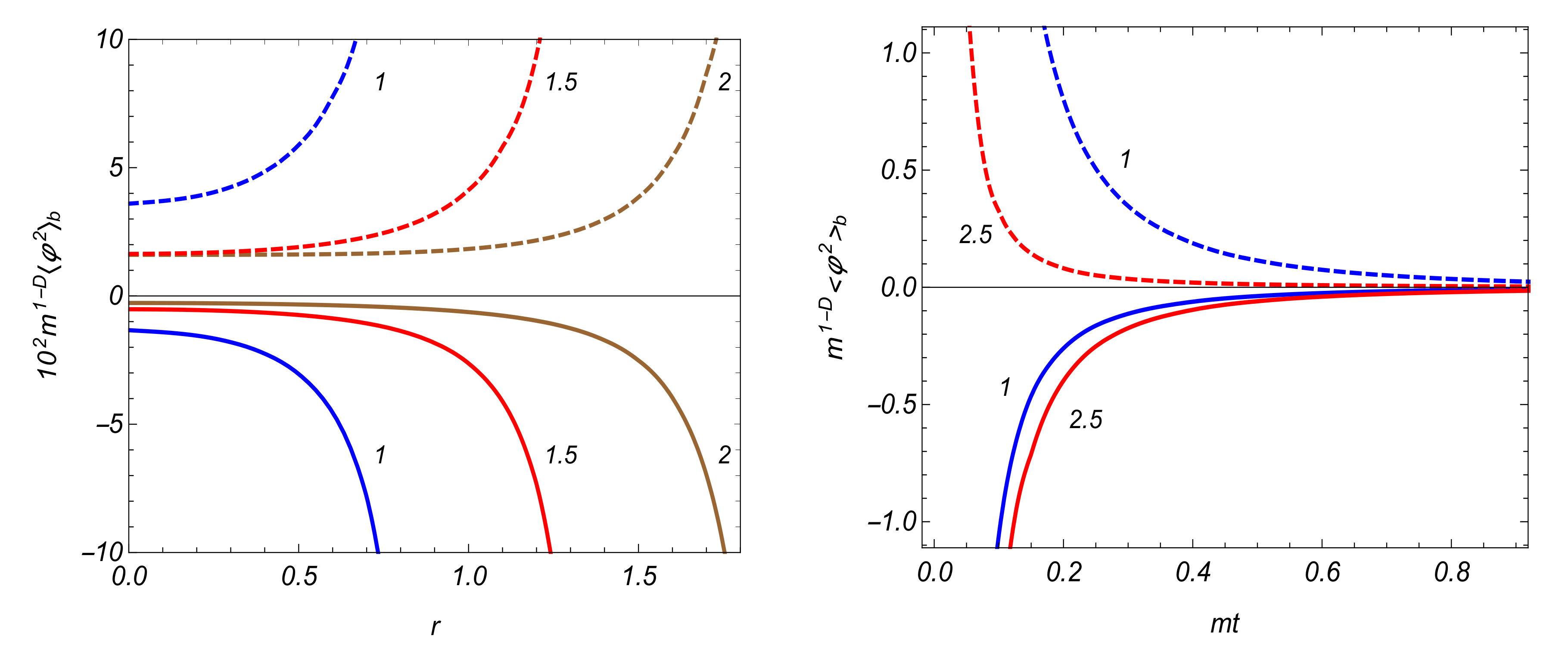
Figure 3.
The sphere-induced contribution in the VEV of the field squared for scalar field versus the Robin coefficient. The graphs are plotted for , and the numbers near the curves correspond to the values of the radial coordinate r.
Figure 3.
The sphere-induced contribution in the VEV of the field squared for scalar field versus the Robin coefficient. The graphs are plotted for , and the numbers near the curves correspond to the values of the radial coordinate r.

Figure 4.
The same as in Figure 2 for the boundary-induced energy density as a function of the radial (left panel) and time (right panel) coordinates in the case of a minimally coupled field.
Figure 4.
The same as in Figure 2 for the boundary-induced energy density as a function of the radial (left panel) and time (right panel) coordinates in the case of a minimally coupled field.
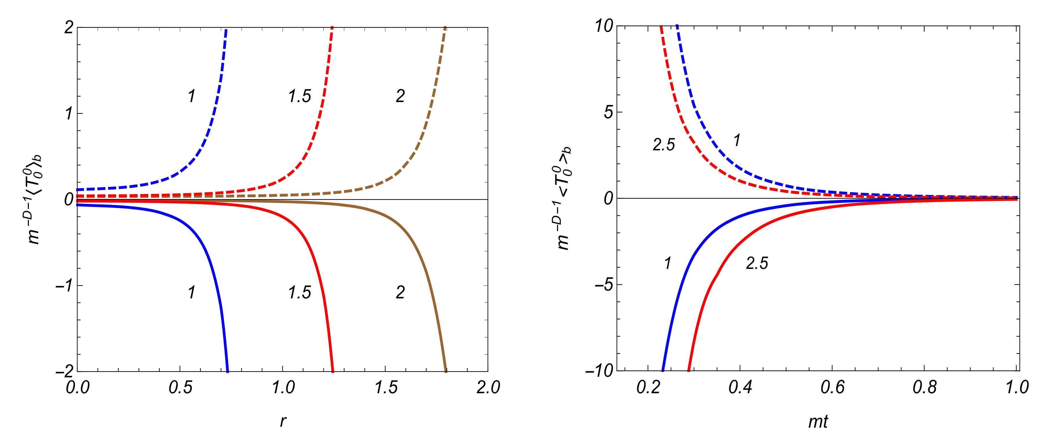
Figure 5.
The same as in Figure 4 for the boundary-induced energy density as a function of the radial (left panel) and time (right panel) coordinates for a conformally coupled field.
Figure 5.
The same as in Figure 4 for the boundary-induced energy density as a function of the radial (left panel) and time (right panel) coordinates for a conformally coupled field.
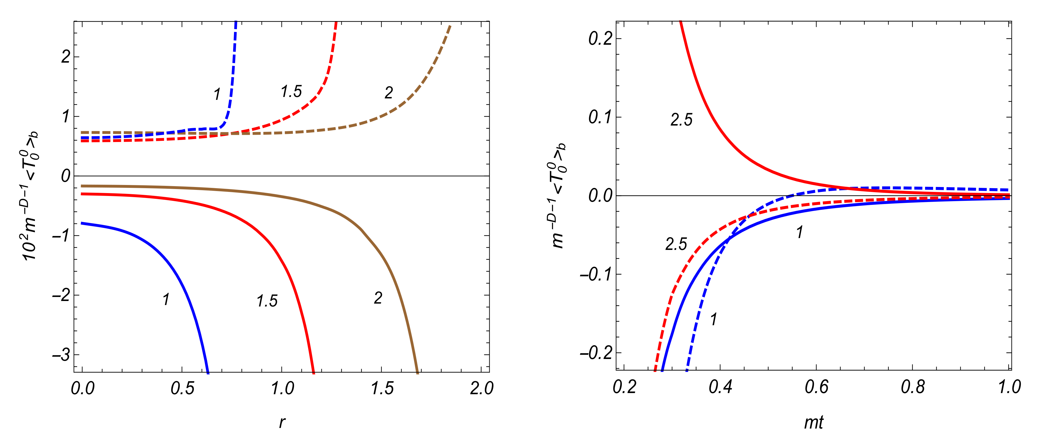
Figure 6.
The same as in Figure 3 for the boundary-induced contribution in the VEV of the energy density for the cases of minimally (left panel) and conformally (right panel) coupled fields.
Figure 6.
The same as in Figure 3 for the boundary-induced contribution in the VEV of the energy density for the cases of minimally (left panel) and conformally (right panel) coupled fields.
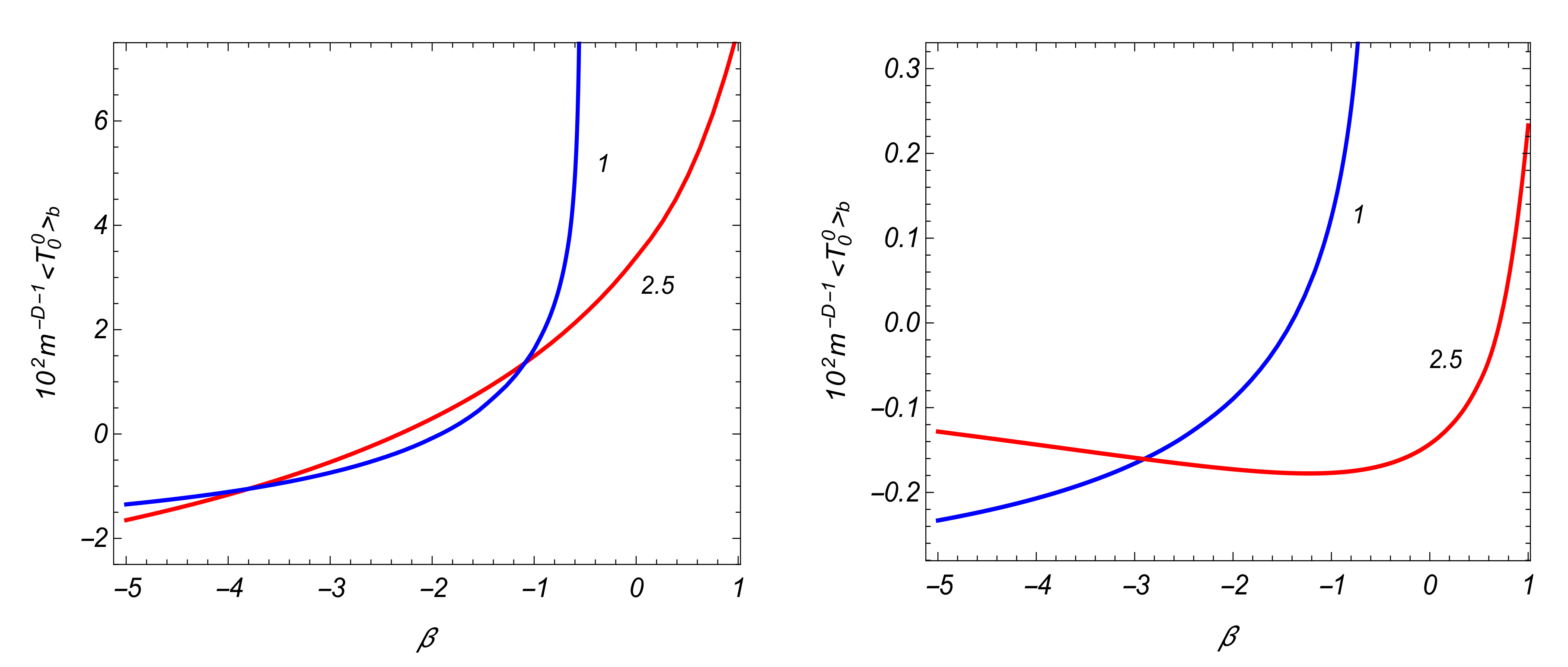
Figure 7.
The same as in Figure 4 for the energy flux density as a function of the radial (left panel) and time (right panel) coordinates.
Figure 7.
The same as in Figure 4 for the energy flux density as a function of the radial (left panel) and time (right panel) coordinates.
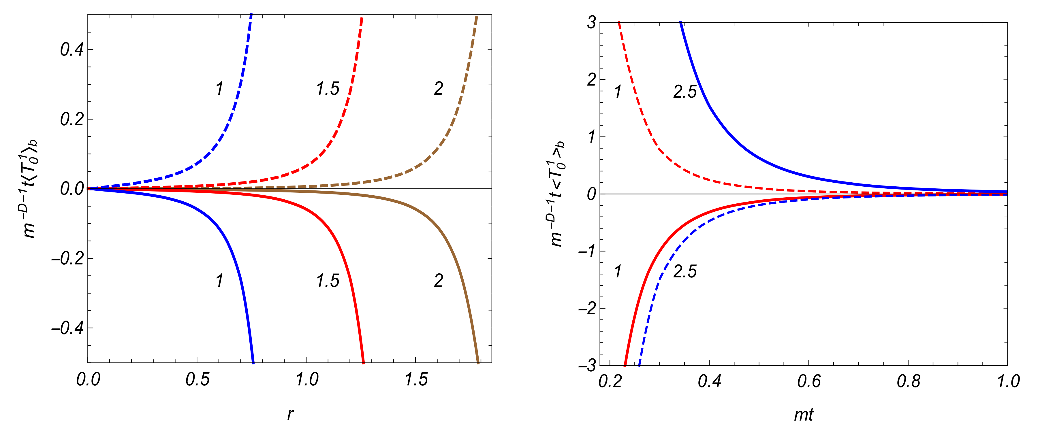
Figure 8.
The same as in Figure 7 for the energy flux density as a function of the radial (left panel) and time (right panel) coordinates in the case of a conformally coupled field.
Figure 8.
The same as in Figure 7 for the energy flux density as a function of the radial (left panel) and time (right panel) coordinates in the case of a conformally coupled field.
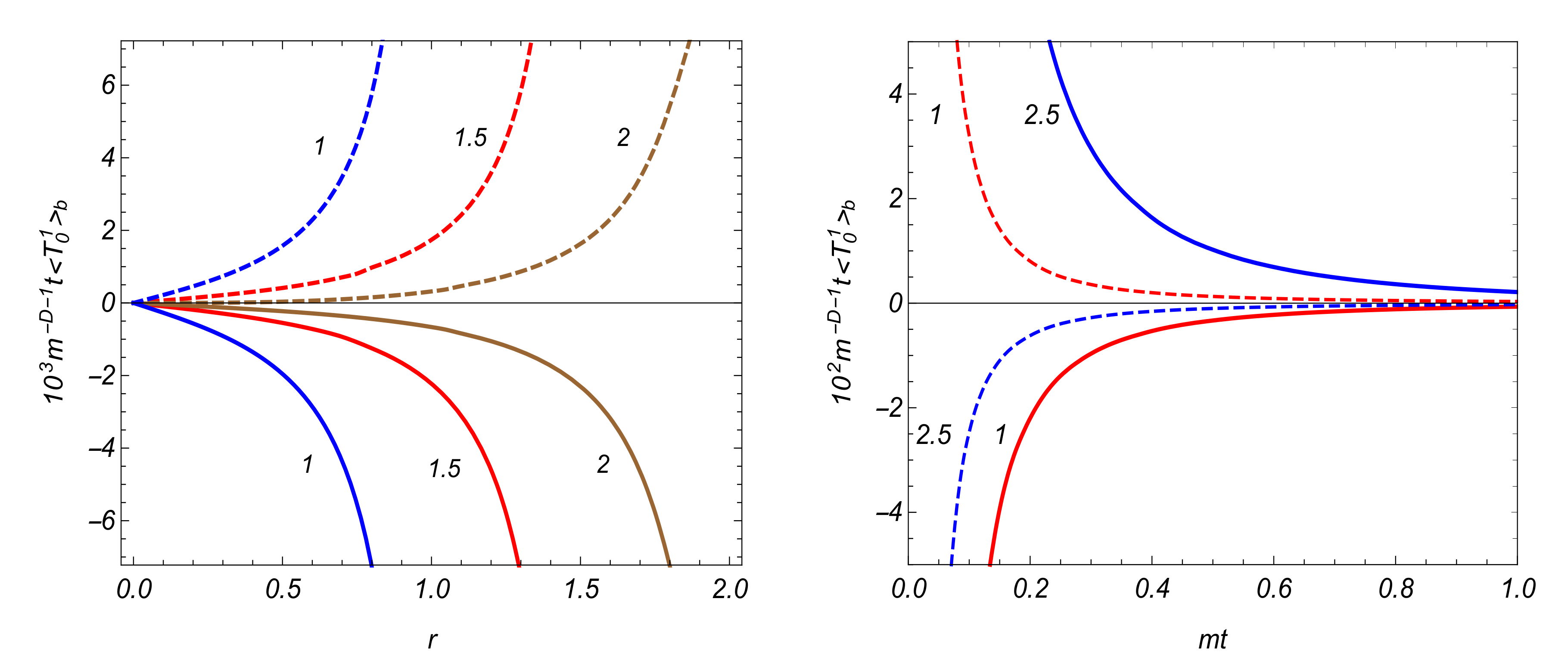
Figure 9.
The same as in Figure 6 for the energy flux density in the cases of minimally (left panel) and conformally (right panel) coupled fields.
Figure 9.
The same as in Figure 6 for the energy flux density in the cases of minimally (left panel) and conformally (right panel) coupled fields.

Figure 10.
The boundary-induced contribution in the VEV of the field squared outside a sphere for scalar field as a function of the radial coordinate. The graphs are plotted for , (numbers near the curves).
Figure 10.
The boundary-induced contribution in the VEV of the field squared outside a sphere for scalar field as a function of the radial coordinate. The graphs are plotted for , (numbers near the curves).
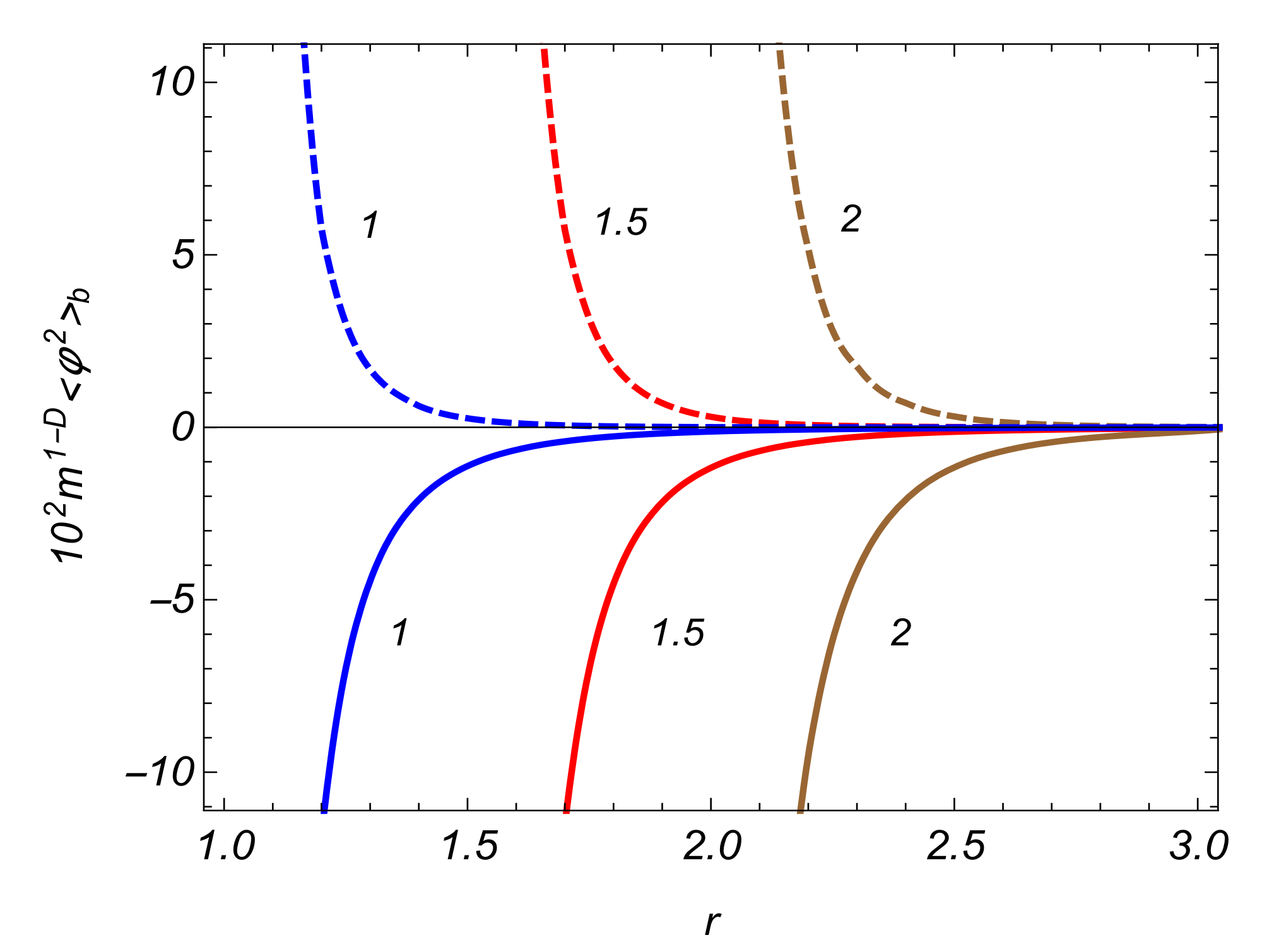
Figure 11.
The boundary-induced contributions in the VEV of the energy density outside the sphere for minimally (left panel) and conformally (right panel) coupled fields. The graphs are plotted for , , and (numbers near the curves).
Figure 11.
The boundary-induced contributions in the VEV of the energy density outside the sphere for minimally (left panel) and conformally (right panel) coupled fields. The graphs are plotted for , , and (numbers near the curves).
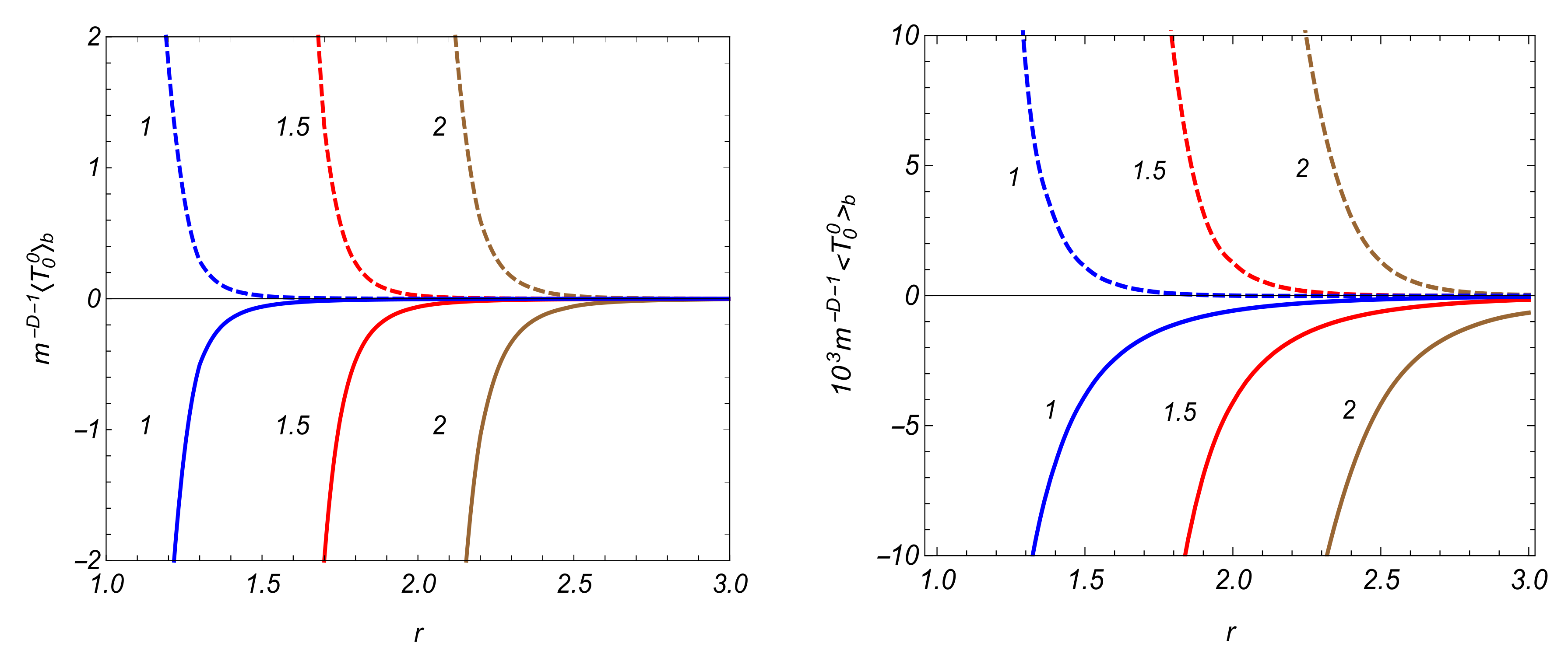
Figure 12.
The same as in Figure 11 for the energy flux density in the cases of minimally (left panel) and conformally (right panel) coupled fields.
Figure 12.
The same as in Figure 11 for the energy flux density in the cases of minimally (left panel) and conformally (right panel) coupled fields.


Table 1.
The critical values of the Robin coefficient for versus the sphere radius.
| 0.5 | 1 | 1.5 | 2 | 4 | 6 | 8 | 10 | |
|---|---|---|---|---|---|---|---|---|
| 0.164 | 0.313 | 0.438 | 0.537 | 0.751 | 0.833 | 0.875 | 0.9 |
© 2020 by the authors. Licensee MDPI, Basel, Switzerland. This article is an open access article distributed under the terms and conditions of the Creative Commons Attribution (CC BY) license (http://creativecommons.org/licenses/by/4.0/).
Share and Cite
MDPI and ACS Style
Saharian, A.A.; Petrosyan, T.A. The Casimir Densities for a Sphere in the Milne Universe. Symmetry 2020, 12, 619. https://doi.org/10.3390/sym12040619
AMA Style
Saharian AA, Petrosyan TA. The Casimir Densities for a Sphere in the Milne Universe. Symmetry. 2020; 12(4):619. https://doi.org/10.3390/sym12040619
Chicago/Turabian StyleSaharian, Aram A., and Tigran A. Petrosyan. 2020. "The Casimir Densities for a Sphere in the Milne Universe" Symmetry 12, no. 4: 619. https://doi.org/10.3390/sym12040619
Note that from the first issue of 2016, this journal uses article numbers instead of page numbers. See further details here.