A Vector Field Texture Generation Method without Convolution Calculation


1
School of Computer Science and Engineering, Northeastern University, Shenyang 110819, China
2
School of Information Science and Technology, Xiamen University Tan Kah Kee College, Zhangzhou 363105, China
3
School of Mathematics and Information Engineering, Longyan University, Longyan 364000, China
4
School of Electronic Engineering, National Formosa University, Yunlin 632, Taiwan
*
Authors to whom correspondence should be addressed.
Symmetry 2020, 12(5), 724; https://doi.org/10.3390/sym12050724
Submission received: 3 March 2020
/
Revised: 1 April 2020
/
Accepted: 8 April 2020
/
Published: 3 May 2020
(This article belongs to the Special Issue Selected Papers from IIKII 2020 Conferences II)
Abstract
:In the LIC algorithm process, symmetrical streamline tracing is used to symmetrically convolve the original values of all the primitive values that pass by to obtain the resulting texture. In this process, streamline tracking and convolution consume a lot of computing resources. To generate more expressive textures for vector fields with less time consumption, a novel method named random increment streamline (RIS) is put forward, which can generate streamline textures without convolution calculations. First, the mesh unit filling preprocessing (MUFP) method is presented to transform an undressed irregular grid into a special kind of regular grid named a “texture pixel”, and the point location and interpolation processes of all sampling points in the texture pixels are calculated before streamline tracking. Second, the random increment streamline method is used to generate line integral convolution style textures without any convolution calculations, thus greatly reducing the algorithm’s time consumption. Third, the vector directions at each point in the static vector field are clearly expressed using the periodic cyclic animation method. Finally, several simplifications of the RIS algorithm are discussed, which help to achieve a better visual effect with faster speed. The programming results show that the method is faster and more applicable than the traditional LIC method and provides clearer expression of the vector field.
1. Introduction
Common vector field visualization techniques include arrow icons, streamlines, path lines, and textures [1]. Compared with other techniques, the biggest merit of textures is that they provide a detailed description of the vector field at the pixel level without losing any valuable information. After long-term evolution, we can classify current texture algorithms into several basic ideas, namely the spot noise method [2], the texture synthesis method [3], the image advection method [4], and the line integral convolution method (LIC) [5]. The LIC method is the most common and important generation method for vector field textures.
In 1993, Cabral et al. [5] proposed the LIC algorithm for the first time. The basic idea of the LIC algorithm is to first cover the vector field with random white noise as the original input texture. Then, starting from a certain primitive value, perform symmetrical tracking in the upstream and downstream directions of the streamline, and then convolve the original primitive values of all sampling points that pass by. The result is the output texture of the sampling point value. After all the primitive values in the vector field are processed, the complete output texture is obtained. Most of the convolution kernel functions used in the convolution process are symmetrical, such as box kernel functions, triangular kernel functions, and Gaussian kernel functions. After years of development, various texture algorithms based on the LIC algorithm have achieved great success, but still have some shortcomings. First, these algorithms are slower due to the streamline tracking and convolution operations. Second, some algorithms [5,6,7] implement certain cyclic animation methods, which can more clearly describe the flow direction in the static vector field. For a static vector field, the vector value at each point in the field does not change with time. If a static texture picture is used for descriptions of the vector value, it is still unknown whether the vector value travels upstream or downstream along the streamline, although the motion tangent of the vector at each point can be clearly expressed. Even though the vector field is static after the application of cyclic animation, the resulting texture is dynamic. The motion of the particles in the loop animation can clearly indicate the true direction of the particles at each point, but there are some shortcomings to these “cyclic animation” methods, such as the need for additional operations and a poor expression ability. Finally, in order to obtain a high-contrast texture [8], additional computation is required, which further reduces the LIC type algorithm’s speed.
To generate vector field textures with better visual effects at a faster speed, the following work is completed in this paper.
First, the mesh unit filling preprocessing (MUFP) method is proposed, which improves the Seed Filling Preprocessing (SFP) method that was proposed in our previous research [9]. The MUFP method uses a regular grid called a “texture pixel” to replace the original irregular grid and preprocesses all sampling points, including point location and interpolation processes, before tracing streamlines. This method significantly accelerates the texture generation.
The second method is called the random increment streamline (RIS) method [10], which can achieve the same visual effect as the LIC algorithm without convolution operations, fundamentally improving the speed of the texture production. This paper will further discuss the RIS algorithm and propose several improvements.
Third, we propose the idea of “periodic circulating animation”, which can better express the vector direction at every point in the static vector field.
Finally, we propose a simplified RIS method, which can further increase the speed of the algorithm and directly obtain high-contrast textures without additional computation.
2. Related Work
As mentioned above, texture generation techniques include several main categories.
The earliest category is the spot noise method [2], based on which there are several modified algorithms, such as the enhanced spot noise [11]. The greatest drawback of these methods is that they do not consider the correlation of adjacent pixels in the upstream or downstream of the same streamline, resulting in rough images.
The second category is the texture synthesis method, which Verma et al. [3] first proposed. Subsequent studies have used techniques, such as “semi-regular textures” [12] and “texture samples” [13], to improve the expressive force and production speed. The main disadvantage of this type of method is that it needs to consider the case of streamline dispersion or convergence, resulting in low efficiency.
The third category is the Image based flow visualization (IBFV) [4] method. In the following research, Jarke [14] et al. applied the IBFV algorithm to a curved grid. Sun Changhui [15] et al. replaced white noise with particles. This method still requires convolutions and sometimes requires data filtering, and so it is also slow. This method has two other disadvantages: it is not suitable for describing a static vector field, and it easily causes visual confusion.
The last category is the LIC method, which is also the most common and important method for generating vector field textures. Cabral et al. [5] first presented this method. The basic idea of the LIC is to use white noise to cover the entire vector field, then trace the streamline and carry out the convolution of the streamline in the plus or minus direction at each sampling point to acquire the output gray value of this point. The convolution operation enables the spatial correlation between adjacent pixels along the streamline direction to be established, while in the vertical streamline direction there is no spatial correlation due to the use of random white noise. This difference can indicate the direction of the flow field. There have been many improvements to the LIC algorithm, among which the Fast Line Integral Convolution (FLIC) [6] algorithm is the most important improvement; the FLIC algorithm increases the speed of the texture generation by an order of magnitude.
Jobard and Lefer [7] proposed a new data structure called the “motion map”, which can be used to draw clear cyclic animations and display the directional information of a steady vector field. The authors of [8] presented the Enhanced Line Integral Convolution (ELIC) method to increase the texture contrast, in which white noise was convolved twice for the purpose of improving the contrast. At the same time, the time consumption was inevitably increased. Wegenkittl et al. proposed two algorithms, Oriented Line Integral Convolution (OLIC) [16] and Fast Oriented Line Integral Convolution (FOLIC) [17], which use dense short streamlines to simulate the LIC effect. In essence, these two algorithms are no longer texture algorithms, rather they generate “pseudo textures”. The advantage of this method is that the computation amount is lower than that of the LIC algorithm, but the disadvantage is that it cannot provide pixel-level flow field details. Another paper presented an improved LIC algorithm [18] that provides the rules for determining the integration step size and interpolation mode according to the vector speed size and the angle between the two vectors. The Unsteady Flow Line Integral Convolution (UFLIC) algorithm was proposed in [19], which follows the traces to realize the visualization of unsteady flow fields.
Interrante [20] and others proposed the volume LIC algorithm to solve the problem of LIC implementation in three-dimensional space. The subsequent series of three-dimensional LIC algorithms can be said to be based on this development. Zhou [21] and others proposed an improved 3D texture algorithm (Enhanced 3D LIC), which performs high-pass filtering on the convolution texture to enhance the contrast, and only displays the area of interest or user features to avoid self-occlusion. Lu [22] and others proposed an enhanced texture advection algorithm, which uses the noise of adjacent sampling points in a three-dimensional vector field to calculate the pseudo gradient and uses the maximum gradient of the pseudo gradient to calculate the texture of adjacent streamlines in order to improve the contrast. In [23], in order to avoid the problem of self-occlusion caused by excessively dense three-dimensional textures, a self-adjusting sparse texture method was proposed to improve the visualization effect. In [24], in order to solve the problem of 3D texture self-occlusion, use of the Halton sequence was proposed to control the distribution of sparse white noise points and remove high-frequency regions by Gaussian filtering to generate sparse 3D textures. In order to further increase the speed, the GPU acceleration algorithm was proposed.
In [25], in order to solve the problem of the low contrast of ordinary LIC textures, where in some cases the color is too concentrated due to uneven changes in the vector field values, improvements in texture enhancement and color enhancement were proposed. In [26], human visual perception theory was introduced into the OLIC algorithm [16] and a particle appearance more suitable for the human eye observation was proposed to improve the visualization effect. In [27], based on the OLIC algorithm, an improved algorithm based on multifrequency sparse noise was proposed. In [28], in order to better express the direction and intensity of the vector field based on the FLIC algorithm, an improved LIC algorithm based on nonlinear gradient color mapping was proposed. In order to improve the speed of the texture generation in [29], parallelization technology was introduced into the FLIC algorithm.
Table 1 summarizes the characteristics of some classic LIC-type texture algorithms. They all have certain disadvantages. As mentioned above, the existing methods of texture generation have problems, such as slow speed, poor visual effects, and poor applicability. Several new methods are discussed below that can significantly improve the speed of texture generation and provide better visuals and greater applicability.
3. Mesh Unit Filling Preprocessing Method
Current visualization studies are generally based on unstructured grids [30] and common unstructured grid generation algorithms, including the Delaunay method [31] and the advancing front method [32]. An irregular grid has many advantages in finite element calculations, such as better coverage of the physical field and strong adaptability. However, for visualization technology, an irregular mesh brings a great deal of trouble.
The first disadvantage of using irregular grids for streamline and pathline tracing is that the time consumption for the point positioning and interpolation calculations is larger than for regular grids. Streamline and pathline integrals often adopt the fourth-order Runge–Kutta (RK4) method [33], as follows:
where pi is the coordinate of current point i and pi+1 is the coordinate of the next point, which is the step length for streamline tracing; v(p) is the vector value of p point, and c1 to c4 are four process parameters.
On the basis of Equation (1), each step of the integration requires four sampling points, and so the point location and interpolation operations for all sampling points are very frequent.
The serial numbers of irregular grid units in the generation process are independent of their coordinate positions, and the two adjacent grid units do not necessarily have continuous serial numbers. In regular grids, each grid unit has exactly the same shape, and the unit’s serial number has a strict relationship with the coordinate position. If the streamline is tracked in a regular grid, based on the coordinates of the sampling point, we can directly know which regular grid cell the sampling point is in. In addition, regular grid cells have a uniform appearance and the interpolation operations are much simpler.
The second disadvantage of using irregular grids for streamline or pathline tracing is that the computation of many point location and interpolation operations is repeated, which also seriously affects the texture generation speed. For example, with a triangular irregular mesh, the area coordinate method is generally used for point positioning and interpolation. Two adjacent sampling points that are adjacent in the same streamline or two sampling points in two adjacent streamlines are likely to be in the same triangular grid, and their area coordinate calculations are likely to contain repeating parts.
To solve the above problems, first an irregular grid can be transformed into a regular grid, and then the point location and interpolation operations can be extracted from the streamline integral process to be completed in advance to avoid repetition.
3.1. Texture Pixel
Based on the previously mentioned discussions, we propose a kind of regular grid named the texture pixel grid. A texture pixel is a small square with fixed side lengths that are parallel to the coordinate axis. All texture pixels combined together can cover the vector field without repetition and omission. Essentially, all texture pixels form a regular grid.
We set the left bottom coordinate of the texture pixel as (x, y) and the square side length of the texture pixel as a. Then, the current texture pixel’s mathematical definition is as follows:
Before we calculate the texture, we point position and interpolate the vertex in the lower left corner of each texture pixel. After all texture pixels are processed in this way, the original irregular grid is transformed into a regular grid that is composed of all texture pixels. Then, in the process of texture generation, the point location and interpolation of each sampling point are no longer conducted according to the original irregular grid unit, but rather are conducted according to the texture pixel, which greatly improves the algorithm’s speed.
The interpolation of the internal sampling points of each texture pixel should use bilinear interpolation [34], as follows:
where a is the edge length of the texture pixel, (x, y) is the coordinate of the sampling point, and v is the physical field value of the sampling point. Here, (xi, yi) are the coordinates of the four vertices in the counterclockwise direction of the texture pixel starting from the lower left corner, and vi is the physical field value of these four vertices.
In practical applications, the shape of a physical field is often not a regular rectangle. At this time, we first need to find a minimum rectangle that can cover the whole physical field, and then according to the edge length of the texture pixel that is set by the user, the minimum rectangle is divided into several rows and columns of small squares. Then, all texture pixels are obtained. To facilitate the subsequent table look-up, the texture pixel’s serial number corresponds directly to its coordinates. We can calculate the serial number of a texture pixel according to
where SN is the ordinal of a texture pixel; x and y are the horizontal and vertical coordinates of the vertex at the bottom left corner of the texture pixel, respectively; xmin and ymin are the horizontal and vertical coordinates of the bottom left corner of the smallest rectangle that can cover the physical field, respectively; lx and ly are the horizontal and vertical resolutions of the final regular grid, respectively; and a is the side length of one texture pixel. Below we discuss how to generate a regular grid made of texture pixels.
3.2. Mesh Unit Filling Preprocessing Method
The core function of the mesh unit filling preprocessing method is to transform the original irregular grid into a regular grid that is composed of texture pixels and to complete the point positioning and interpolation calculations for all vertices of all texture pixels. Based on the order in which this transformation is accomplished, the efficiency is quite different.
Regarding methods used for the point location and interpolation of a sample point, the walk-through method [35] is a mature method, but this method is not highly efficient. The scan line seed fill method is used in [36], which can preprocess all grid cells at one time. The basic idea of this method is to take a certain texture pixel as the seed point, point locate and interpolate all texture pixels to the left and right successively, and stop when both sides meet the grid boundary, at which time a horizontal scanning line segment is formed. The next step is to recursively scan the two top and bottom adjacent scan lines. At the end of the recursion, all texture pixels are preprocessed. The reason for the recursion is that the original grid may be a multiple-connected domain.
The Seed Filling Preprocessing (SFP) [9] method that was proposed in our previous work improves the scan line seed fill method, in which the preprocessing of the vector field is no longer completed at once, but one independent grid unit is processed at a time. Within each grid cell, we still use the recursive idea to preprocess all texture pixels. When all the mesh cells are processed, the whole mesh is converted into many texture pixels. This improves the speed because the grids that are adjacent can be neglected.
The analysis shows that recursion is not optimal for triangular grid cells (and other types of grid cells). First, because the interior of a triangular grid unit is definitely a simply connected domain, no recursion is required. Second, when the number of recursive layers is large, the efficiency of the recursive algorithm decreases sharply. Therefore, in mesh unit filling preprocessing, we replace the recursive idea with the general cyclic idea and further improve the pretreatment efficiency.
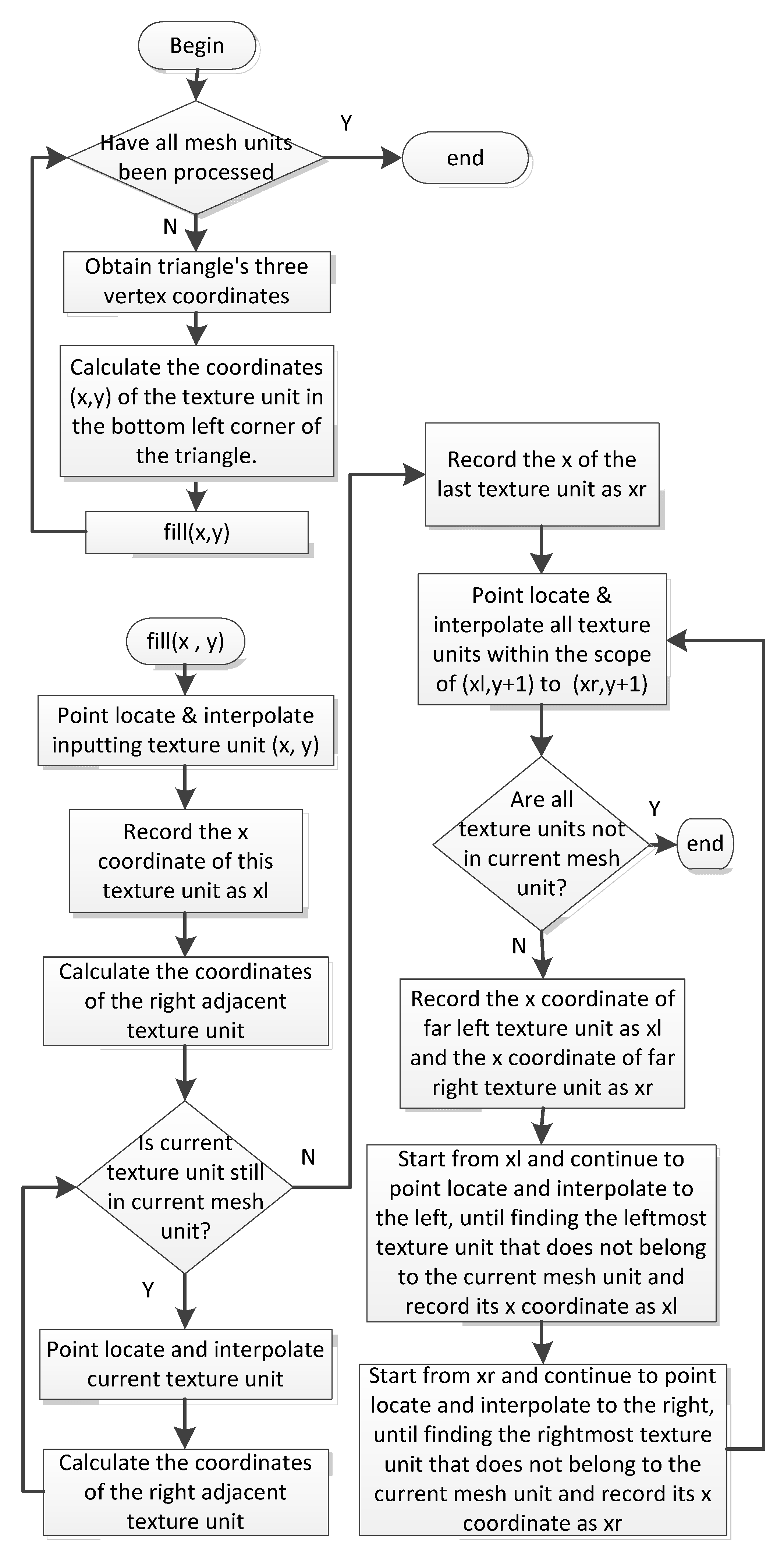
The complete program flow chart of the mesh unit filling preprocessing method is shown in Figure 1. The top part of Figure 1 shows the whole course of the mesh unit filling preprocessing, and the essential idea is to handle each mesh unit on the basis of the unit number. The lower part describes the processing in a mesh unit, which is basically a cyclic process.
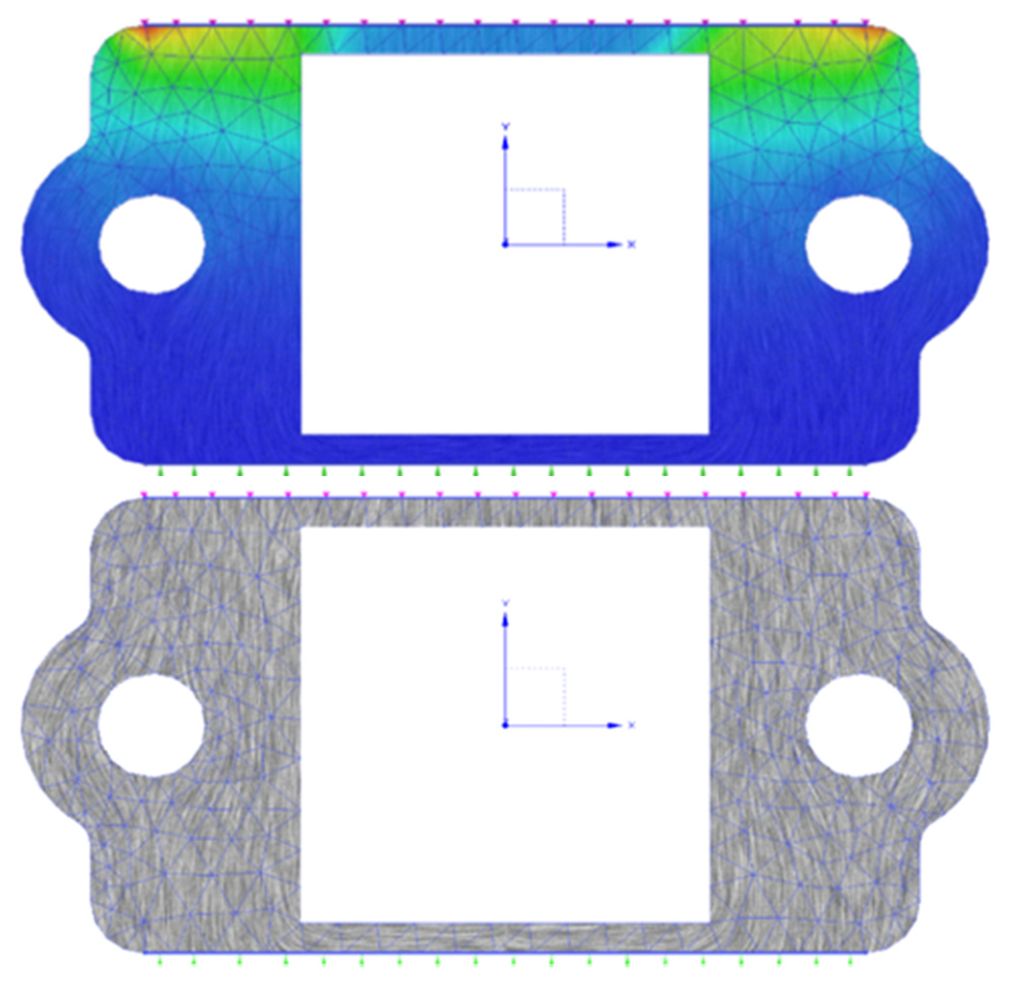
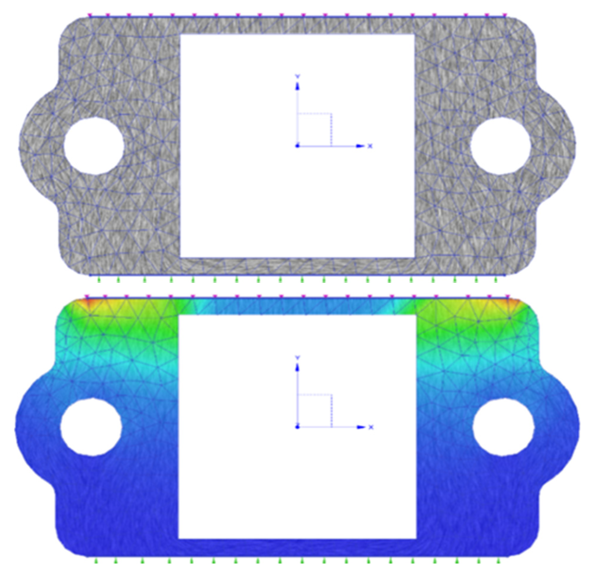
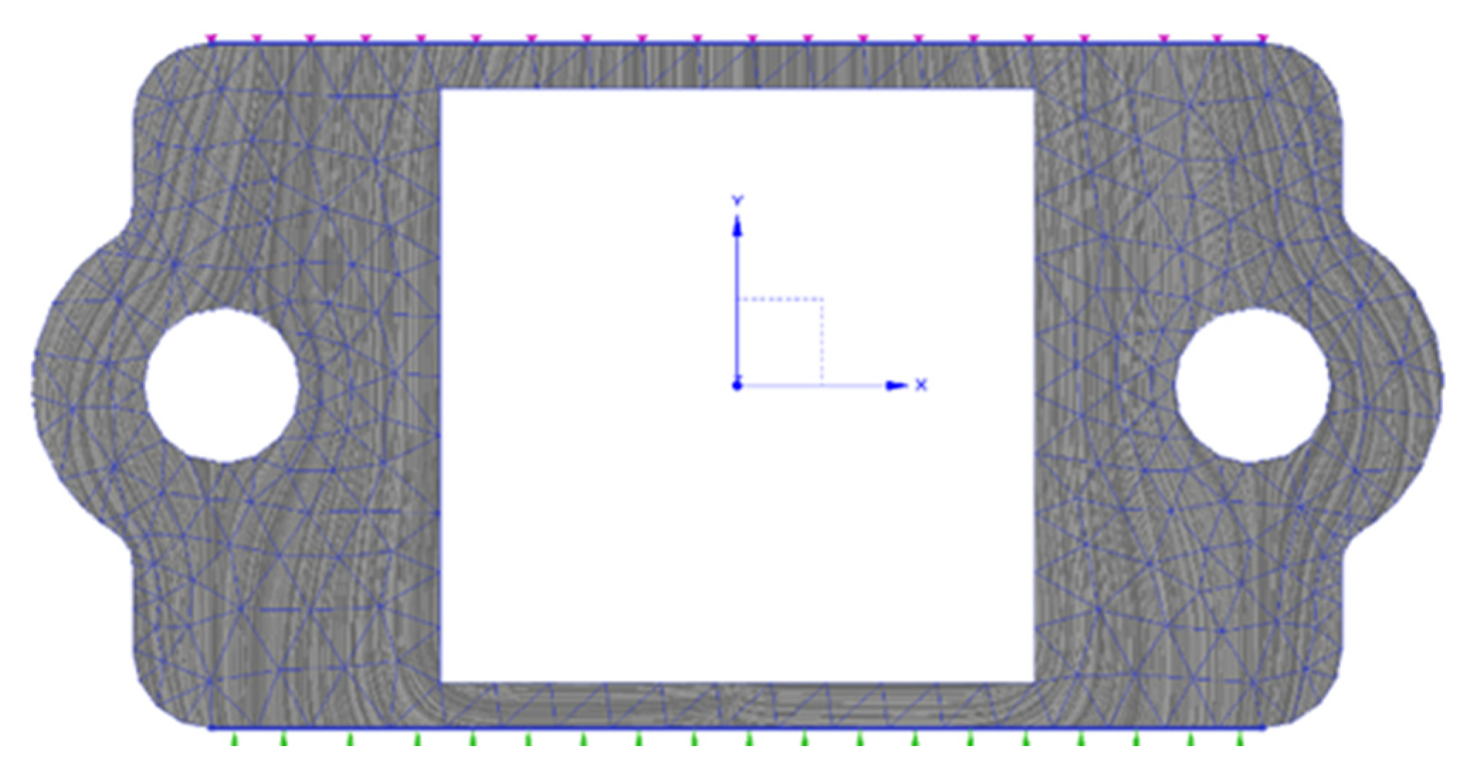
Figure 2 shows an example of a texture in an irregular triangular grid. The amount of texture pixels is 533 × 800 = 426,400, while the amount of mesh units is 2740. When we adopted the walk-through algorithm, the time consumption of calculation all texture pixels was 15.426 s, the SFP method took 3.869 s, and the MUFP method took 3.520 s. Obviously, the time efficiency of the MUFP algorithm is much better than the walk-through and SFP methods.
To better compare the performance of the three algorithms, we use the physical field in Figure 2 to set different grid cell numbers and texture pixel resolutions. Then, the walk-through, SFP, and MUFP methods are used to complete the point location and interpolation of all texture pixels. The time that is taken is shown in Table 2.
As can be clearly seen from Table 2, compared with the walk-through method, the time efficiency of the MUFP method is significantly improved, especially when the number of grid cells and the number of texture pixels increase simultaneously. Meanwhile, the time efficiency of the walk-through method is too low to be tolerated. In addition, it can also be seen from Table 2 that the time consumption of the MUFP method has a weak relationship with the number of grid cells, and it mainly increases in direct proportion with the increase of the texture pixels.
An interesting phenomenon is that with the same texture pixel resolution, the time consumption of the SFP algorithm decreases as the amount of mesh units increases. This is mainly because the area of each grid unit decreases as the amount of grid units increases, resulting in an increase in the number of texture pixels in each grid cell. The SFP algorithm has to perform more recursive operations, meaning the time consumption increases. In conclusion, the MUFP method is significantly better than the walk-through and SFP methods when preprocessing irregular grids.
4. Random Increment Streamline Method
4.1. Basic Idea
The traditional LIC [5] method uses white noise as the input image to overlay the entire vector field. To calculate the output texture gray value of a sampling point, the LIC algorithm traces the streamline for a distance upstream and downstream based on the value of the vector field at that sampling point. Then, the input gray values of all points that the short streamline segment passes through are convolved to determine the output pixel gray value of this sampling point. The process can be described as
where F′(x, y) is the final output texture primitive value at the point (x, y), F(⌊Pi⌋) is the input primitive value at point Pi passed by the streamline tracking, hi is the weight point at the time of convolution, L is the number of streamline tracking steps in the forward direction, and L′ is the number of streamline tracking steps in the reverse direction.
In general, the number of tracking steps in the two directions of the streamline is the same. In other words, L and L′ are equal in Equation (5). In addition, we calculate the weight of each sampling point by the convolution kernel function k, then Equation (5) can be simplified into the following formula:
where T(x0) is the output texture gray value of the sampling point x0, I(xi) is the input gray value of the point xi, L is the tracing length of one side, and k(xi) is the convolution kernel function.
According to Equation (6), the convolution calculations of two adjacent sampling points on the same streamline are very similar, with only one factor difference. Relative to sampling point xm, the convolution calculation of xm+1 no longer contains the factor xm−L, but rather it contains an extra factor xm−1−L. Based on this idea, the FLIC [6] algorithm uses faster calculation to improve the algorithm speed, as follows:
where xm is a sampling point on the streamline whose gray value has been calculated, and xm+1 is the next adjacent sampling point on the streamline. Please note that the letters used in Equation (7) and the literature [6] are slightly different in order to ensure consistency in the discussion in this article.
In our previous work, we proposed the RIS [10] algorithm, which can obtain textures that are similar to the LIC algorithm without convolution. In the RIS algorithm, two important formulas are used, as follows:
We use Equation (8) to calculate the gray value of each streamline’s seed-point, where L is the step length for unilateral convolution. Because RIS does not actually execute the convolution, L is simply a parameter to control the output image’s effect. The asymptotic normal distribution (AND) function returns a random floating point number. In the AND function, 127.5 is the mathematical expectation, while the second parameter is the variance. By using Equation (9), we can acquire the output gray value of the streamline’s subsequent pixels. For uniform distribution (UD), the two parameters of the function are upper and lower bounds, while the return value of the function is a random number that complies with UD distribution. Equation (8) is equivalent to Equation (6), and Equation (9) is equivalent to Equation (7). The specific proof process is as follows.
To prove that these formulas are equal, two facts need to be clarified. First, all LIC methods use white noise as the input texture, i.e., I(xi) − U[0, 255]. Second, in various LIC methods, the convolution kernel function k(xi) has different forms, but in the FLIC method, only the box kernel function was used. Our RIS method also uses the box kernel function only.
Let’s prove that Equation (8) is equivalent to Equation (6).
Prove:
Since ,
hence, and
.
Since in Equation (2) is constant, .
Hence, .
That is, is the sample mean of (2L + 1) independent and uniformly distributed random variables .
Hence, from the central-limit theorem, obeys an asymptotic normal distribution; that is,
and .
Hence, Equation (2) is equivalent to ,
thereby completing the proof.
Next, we will prove that Equation (9) is equivalent to Equation (7).
Proof:
Since in Equation (3) and are both white noise,
hence, and
and they are independent of each other.
Hence, .
Furthermore, since ,
hence,
.
That is, Equation (2) is equivalent to ,
According to the foregoing proof, Equation (8) can calculate the gray value of each streamline’s seed point and Equation (9) can calculate gray values of follow-up points along the streamline. Finally, we get a texture very akin to LIC. The UD function in Equation (9) can be directly obtained by using the random function in the programming language. According to the mathematical definition of an asymptotic normal distribution, we need to generate m different random numbers with a uniform distribution within the range of 0–255 and then average these numbers to obtain the AND function’s result. In programming, we find that when m = 12, the resulting image is very analogous to the LIC image.
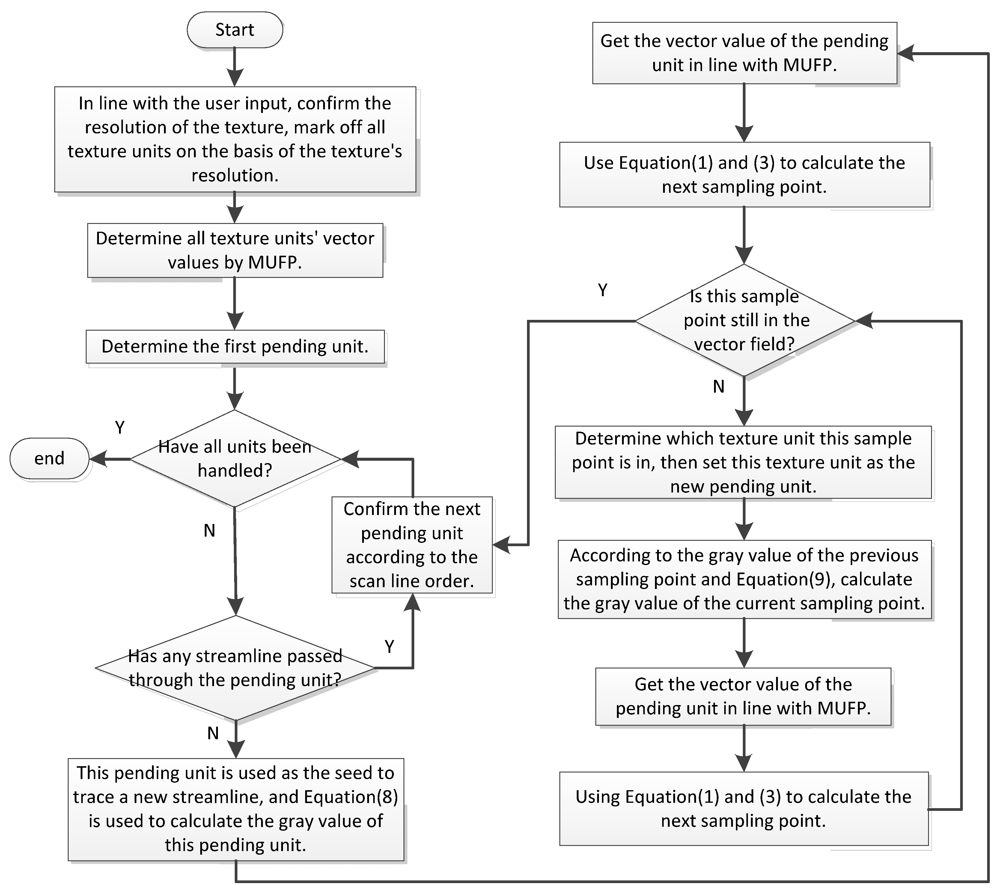
Figure 3 shows the procedure flow chart of the RIS method. The basic processes for RIS and FLIC is similar, with three important improvements. Firstly, the MUFP algorithm is used to complete the localization and interpolation of all texture pixels in advance. Secondly, Equation (8) instead of white noise is used to calculate the pixel values of the seed point of each streamline. Third, Equation (9) is used to calculate the gray value of the follow-up sample points along the streamline. Through these improvements, RIS has a much higher time efficiency than FLIC.
Similar to the LIC algorithm, in the RIS algorithm, several streamlines may cross the same texture pixel. Only retain the gray value of the first or the last streamline should be retained, or the gray values of multiple streamlines can be accumulated and then normalized at a later stage.
We can use Equation (10) to get the color texture, where the color value can express the size of the vector field.
In Equation (10), Tout is the colored texture, TLIC is the original texture obtained by the RIS method, Tmag is the contour graph drawn in line with the vector field modulus value, and t is the mixed parameter. The larger the t, the higher influence the contour graph is. The smaller the t, the more obvious the original texture is.
Figure 4, Figure 5 and Figure 6 show the textures that are obtained by using the LIC, FLIC, and RIS algorithms for the same group of data. All of the above three algorithms adopt the MUFP method for point positioning and interpolation and the RK4 method for streamline tracking. Figure 4 is generated by the LIC, Figure 5 by the FLIC, and Figure 6 by the RIS. The gray textures are on the top and color textures are on the bottom. It can be seen that the resulting textures are very similar.
4.2. Periodic Circulating Animation
The textures that are generated according to the above method form a static pattern, and so only the size and direction information of the vector field can be described, not the directional information of the particle motion. The LIC algorithm and its derivative algorithm propose a variety of circulating animation methods to compensate for this defect. The purpose of these methods is to move the pixels downstream along the streamline, thus using animation to describe the directional information of the particle. These methods include periodic motion filters [5], the convolution kernel function in the LIC, the frame blending method in the FLIC [16], and the motion map method [7]. The main feature of the motion map method is that the color values of all pixel points on the streamline are no longer calculated using convolutions, but rather that they are assigned by directly selecting a certain color from a precalculated “color table” according to certain rules. This form of circular animation has high definition, but it poses two problems. First, because adjacent streamlines are assigned according to the color in the same color table, a certain correlation can be introduced in the direction of vertical streamlines, and distortions may occur in some cases. Second, the color values of pixels on the streamline are assigned using the color table, which is irrelevant to the actual vector information at the point, and sometimes misleads users.
Therefore, in the RIS, we adopted a simpler and more efficient way to implement circulating animation, which is called the periodic circulating animation method, the steps of which are as follows.
Step 1: Divide each streamline in the RIS texture into several segments of the same length, with no less than 3 segments.
Step 2: The N-frame texture image is formed. In the i-th frame, the i-th texture pixel in each streamline segment is replaced by a special particle.
Step 3: The N-frame animation is played in a loop, and the whole animation reflects the vector motion direction at each pixel.
For the visual effect, the special particles in step 2 should have special colors. For example, for gray textures, a red pixel should be used, and for color textures, a black pixel should be used.
When the animation is played, all stream segments will release special particles at the same time, which will cause obvious aliasing artifacts. To solve this distortion problem, we generate a random number m within the range of 0-(len-1) for each stream segment and then loop the current stream segment to frame m in advance. The initial states of the different streamline segments are no longer the same, thus solving the aliasing artifacts problem.
Figure 7 shows a frame in the periodic animation of the RIS color texture, in which some pure black particles are used instead of the original color pixels.
5. Simplified RIS Algorithm
Using the above Equations (8) and (9), we can obtain a texture that is very similar to the visual effect from the LIC. After analysis, we find that we can further reduce the time costs of the algorithm without reducing the texture effects and can produce some special visual effects. We use
instead of Equation (8) to assign random gray values to the seed points of each new streamline, where the function UD has the same meaning as in Equation (8) above, and r is a control parameter.
To further increase the speed, we use
instead of Equation (9) to calculate the gray value of the streamline’s follow-up sample points. This means that all pixel points on the same streamline have the same gray value without any change. We call this algorithm using Equations (11) and (12) the simplified RIS (SRIS) algorithm.
According to the above discussion, we know that the asymptotic normal distribution function needs to calculate 12 independent random numbers with a uniform distribution, while the uniform distribution function only needs to perform the calculation once, which obviously reduces the time consumption. If Equation (12) is used instead of Equation (9), the color calculation of the subsequent sampling points of the streamline are simply cancelled, which will obviously improve the speed of the algorithm.
The other advantage of using Equation (11) instead of Equation (8) is that we can easily achieve high contrast without increasing the computation by just adjusting the parameter r. Figure 8a shows the texture that is drawn using Equations (8) and (9), which is very similar to the traditional LIC algorithm. The following three pictures are drawn with Equations (11) and (9), and the parameter r is set to 30, 50, and 90. It can be seen that due to the increasing difference in the gray values of the seed points of different streamlines, the final texture has high contrast.
The textures that are generated by the SRIS with Equations (11) and (12) are shown in Figure 9. It can be seen that there is no loss in the description of the vector field direction or size information. Furthermore, to some extent, the description of the directional information becomes clearer, and the time costs of the RIS algorithm are greatly reduced.
Furthermore, we adjust the parameter r to improve the contrast of the texture image, which achieves a similar high-contrast texture effect to that in [8]. As shown in Figure 10, we can obtain a clearer vector field expression without any additional operations.
It should be noted that when using Equation (12), since all the streamlines in the texture have a fixed color, aliasing artifacts may occur. The reason why aliasing of the artifacts does not occur in the LIC algorithm is that the gray values of each streamline in the LIC algorithm constantly and randomly change, while the gray values of each streamline in the SRIS algorithm are always fixed, thus resulting in aliasing artifacts. If this distortion needs to be avoided, Equation (9) can be reused to avoid aliasing artifacts, as in Figure 8.
6. Results and Discussion
According to the above ideas, we completed the program, with the experimental results verifying that the algorithm is effective.
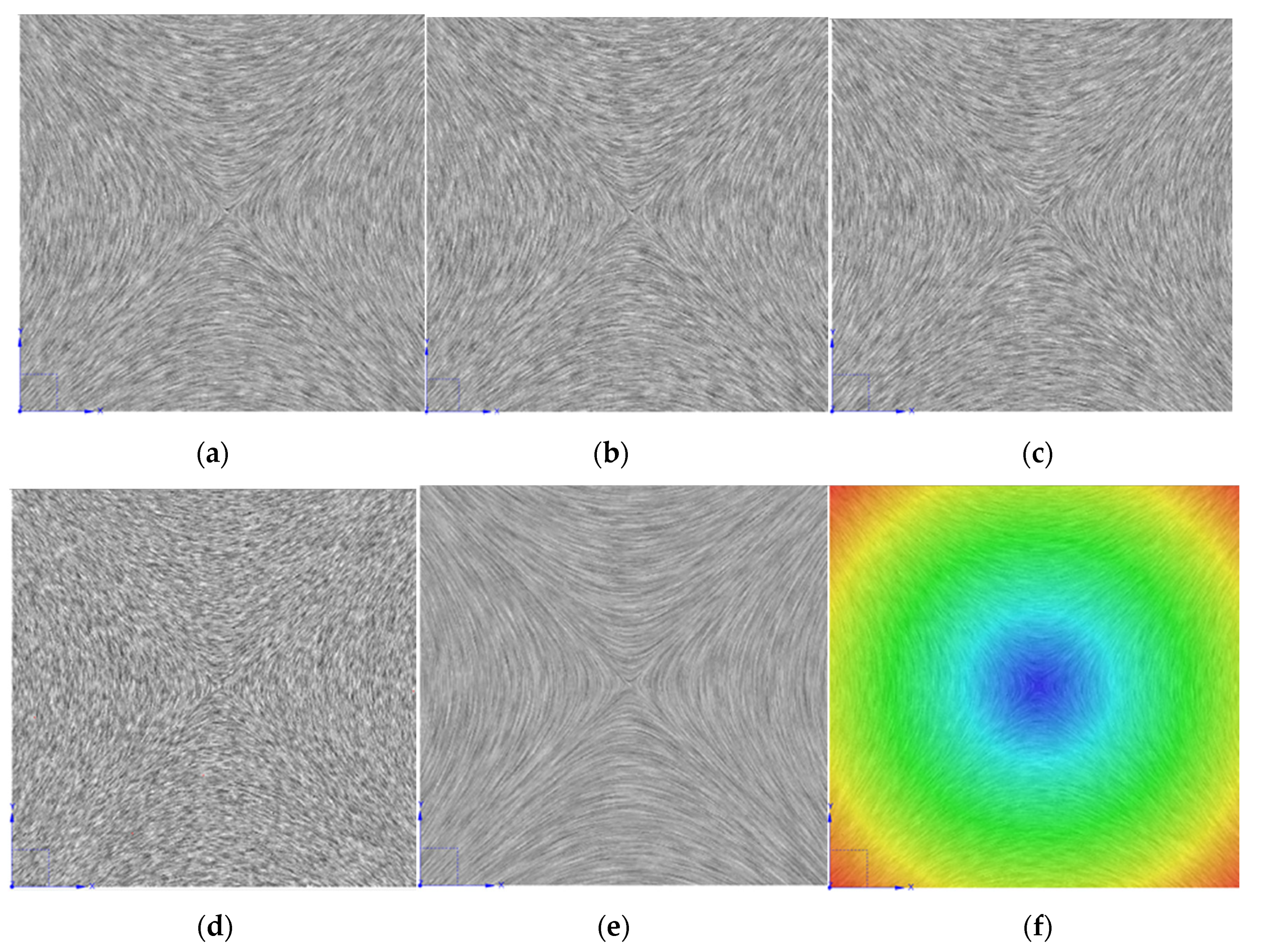
Figure 11 shows a set of textures drawn according to artificial concentric circle vector field data. Figure 11a is drawn using the LIC algorithm, Figure 11b is drawn using the FLIC algorithm, and Figure 11c is drawn using the RIS algorithm. The one-sided convolution length L is the parameter L in Equation (8), which is set to 10. You can see that the appearance of the RIS texture is basically the same as the traditional LIC algorithm. In order to further verify the effect of the RIS algorithm, the parameters for L in Equation (8) are set to 5 and 20, respectively, and Figure 11d,e are obtained. Short texture and long texture effects are achieved. Figure 11f is the RIS texture obtained using Equation (10).
Figure 12 shows a set of textures drawn based on an artificial saddle-shaped vector field data. The algorithm and parameters used for specific rendering are exactly the same as those in Figure 11.
Figure 13 shows the RIS texture (Figure 13a) and SRIS texture (Figure 13b,c) of a set of wind field data. It can be seen that the gray texture of SRIS can more clearly describe the directional distribution of the wind speeds than the RIS texture. In the color texture, different colors can be used to express the modulus of the wind speed, such that the wind speed can be directly expressed.
We used the other two groups of wind field data to draw two sets of textures, as shown in Figure 14 and Figure 15.
In this part, a defect of the SRIS algorithm is discussed. In some cases, the gray texture generated by the SRIS algorithm will produce more obvious artifacts, such as in Figure 9, Figure 10, Figure 13b, Figure 14b and Figure 15b. It is found in the analysis that when some adjacent streamlines occur along the X-axis or Y-axis direction of the screen, a vertical or horizontal line segment appears at the same time in these adjacent streamlines. Artifacts are generated in the perpendicular direction. The reason why such artifacts do not occur in the RIS algorithm is that the gray level on the streamline in the RIS algorithm changes constantly and randomly, and this change offsets the effect of the artifact. Unfortunately, the nature of this algorithm cannot remove this artifact because only one gray level is used on the SRIS streamline, but color textures can be used to cover this artifact. For example, in the colored textures in Figure 13c, Figure 14c and Figure 15c, such artifacts can hardly be found.
For comparison, we use the LIC, FLIC, RIS, and SRIS algorithms to draw the same texture. All of the algorithms adopt the MUFP method for preprocessing and the RK4 method for tracking. The time consumption of the four color textures that are generated by the four algorithms is shown in Table 3. It can be seen from Table 3 that the time efficiencies of the RIS and SRIS algorithms are much faster than those of the LIC and FLIC methods.
It can be seen from the above results that the RIS and SRIS methods can greatly improve the texture generating speed and have stronger adaptability and more expressiveness. When we use the SRIS to calculate the texture, the time consumption is greatly reduced and the resulting long streamline texture also provides a better vector field direction expression. Furthermore, we can simply adjust the parameter r in Equation (11) without any extra computation, obtaining a texture pattern with higher contrast.
Finally, the differences between RIS algorithms and traditional LIC texture algorithms are summarized, along with an explanation of why RIS algorithms are faster than FLIC algorithms. In the LIC algorithm, the output texture value of each sampling point is tracked L steps in the upstream and downstream directions according to the vector field value at that point, and then the original white noise of the 2L + 1 sampling points that were passed through is input into gray degree values that are weighted and averaged. In this calculation process, there are two time-consuming processes—streamline tracking and weighted averaging. In the FLIC algorithm, the reason why the speed can be increased by an order of magnitude is because the FLIC algorithm simplifies the weighted average process. In the original LIC, in order to calculate the average value, we have to perform 2L + 1 summation operation. In the FLIC algorithm, the sum of the adjacent previous points is subtracted from the gray value of the most remote sampling point upstream of the streamline, along with the gray value of the most remote sampling point downstream of the streamline. The sum of the current points essentially simplifies the 2L + 1 summation operation into one subtraction operation and one addition operation, which greatly saves time. The AND function used in Equation (8) and the UD used in Equation (9) in the RIS algorithm are calculated in advance at the very beginning of the algorithm. In the process of actual tracking on the streamline, Equation (7) can be accomplished by simply reading the table. The operation of Equation (8) requires only one additional operation based on the meter reading. This fundamentally reduces the amount of calculations, meaning it is faster than the FLIC algorithm. The MUFP method is used to transform an irregular grid into a regular grid, while interpolation of the most time-consuming sampling vector field values in the streamline tracking process is completed in advance. This greatly increases the speed of the streamline tracking. Therefore, the RIS algorithm greatly simplifies two of the most time-consuming operations in the traditional LIC algorithm, which effectively improves the texture generation speed.
In future work, we will continue to improve the RIS algorithm so that it can be applied in more scenarios, including alterable velocity texture and textures in three dimensions. We will also study the application of textures in tensor field visualization [37].
Author Contributions
Conceptualization, X.D.; methodology, X.D. and H.L.; software, X.D. and H.L.; validation, H.-W.T., T.-H.M. and H.L.; formal analysis, X.D., H.-W.T., T.-H.M. and H.L.; investigation, T.-H.M.; resources, H.-W.T. and T.-H.M.; data curation, T.-H.M. and X.D.; writing—original draft preparation, X.D.; writing—review and editing, H.-W.T. and H.L.; visualization, X.D. and H.L.; supevision, H.L. and H.-W.T.; project administration, X.D.; funding acquisition, X.D. All authors have read and agreed to the published version of the manuscript.
Funding
This work was supported by Natural Science Foundation of Fujian, China (Project No. 2018J01101).
Conflicts of Interest
The authors declare no conflict of interest.
References
- David, H.L.; Robert, M.K.; Cullen, D.J.; Davidson, J.S.; Timothy, S.M.; Marco, D.S.; William, H.W.; Michael, J.T. Comparing 2D Vector Field Visualization Methods: A User Study. IEEE Trans. Vis. Comput. Graph. 2005, 11, 59–70. [Google Scholar]
- Van, W.; Jarke, J. Spot noise: Texture synthesis for data visualization. In Proceedings of the ACM Siggraph, New York, NY, USA, 3 July 1991; pp. 309–318. [Google Scholar]
- Vivek, V.; David, K.; Alex, P. PLIC: Bridging the Gap between Streamlines and LIC. In Proceedings of the IEEE Visualization, San Francisco, CA, USA, 24–29 October 1999; pp. 341–348. [Google Scholar]
- Van, W.; Jarke, J. Image based flow visualization. ACM Trans. Graph. 2002, 3, 745–754. [Google Scholar]
- Brian, C.; Leith, L. Imaging vector fields using line integral convolution. In Proceedings of the ACM Siggraph, Anaheim, CA, USA, 2–6 August 1993; pp. 263–270. [Google Scholar]
- Detlev, S.; Hege, H.C. Fast and resolution independent line integral convolution. In Proceedings of the ACM Siggraph, Los Angeles, CA, USA, 6–11 August 1995; pp. 249–256. [Google Scholar]
- Bruno, J.; Wilfrid, L. The Motion Map: Efficient Computation of Steady Flow Animations. In Proceedings of the IEEE Visualization’97, Phoenix, AZ, USA, 19–24 October 1997; pp. 323–328. [Google Scholar]
- Arthur, O.; David, K. Enhanced line integral convolution with flow feature detection. In Proceedings of the IS&T/SPIE Electronic Imaging, San Jose, CA, USA, 9–13 June 1997; pp. 206–217. [Google Scholar]
- Du, X.F.; Liu, H.L. Seed Filling Preprocessing: A universal visualization preprocessing method in irregular grids. In Proceedings of the 30th Chinese Control and Decision Conference (CCDC2018), Shenyang, China, 9–11 June 2018; pp. 4378–4382. [Google Scholar]
- Du, X.F. A New Texture Generating Algorithm: Random Increment Streamline Method. In Proceedings of the 37th Chinese Control Conference (CCC2018), Wuhan, China, 25–27 July 2018; pp. 1679–1684. [Google Scholar]
- De, L.; Willem, C.; Van, W.; Jarke, J. Enhanced spot noise for vector field visualization. In Proceedings of the IEEE Visualization, Atlanta, GA, USA, 29 October–3 November 1995; pp. 233–239. [Google Scholar]
- Wang, B.; Wang, W.P.; Yong, J.H.; Sun, J.G. Flow Visualization by Near-Regular Texture Synthesis. J. Comput. Aided Des. Comput. Graph. 2005, 8, 1678–1685. [Google Scholar]
- Lin, L.L.; Yang, G.; Huang, H.D.; Liu, X.H.; Wu, E.H. Vector Field Visualization Based on Texture Synthesis. J. Comput. Aided Des. Comput. Graph. 2006, 11, 1677–1682. [Google Scholar]
- Jarke, J.; Van, W. Image Based Flow Visualization for Curved Surfaces. In Proceedings of the IEEE VIS 2003, Seattle, WA, USA, 19–24 October 2003; pp. 123–130. [Google Scholar]
- Sun, C.H.; Fan, Y.; Li, Q.; Huang, W. Enhanced IBFV 2D vector field visualization. J. Image Graph. 2011, 6, 1064–1069. [Google Scholar]
- Rainer, W.; Eduard, G. Animating flow fields: Rendering of oriented line integral convolution. In Proceedings of the IEEE Computer Animation, Geneva, Switzerland, 5–6 June 1997; pp. 15–21. [Google Scholar]
- Rainer, W.; Eduard, G. Fast Oriented Line Integral Convolution for Vector Field Visualization via the Internet. In Proceedings of the IEEE Visualization, Phoenix, AZ, USA, 19–24 October 1997; pp. 309–316. [Google Scholar]
- Qin, X.J.; Fang, X.; Chen, L.H.; Zheng, H.B.; Ma, J.; Zhang, M.Y. A Line Integral Convolution Method with Dynamically Determining Step Size and Interpolation Mode for Vector Field Visualization. IEEE Access 2019, 7, 19414–19422. [Google Scholar] [CrossRef]
- Shen, H.-W.; David, L.; Kao, A. New Line Integral Convolution Algorithm for Visualizing Time-Varying Flow Fields. IEEE Trans. Vis. Comput. Graph. 1998, 4, 98–108. [Google Scholar] [CrossRef] [Green Version]
- Interrante, V.; Grosch, C. Strategies for effectively visualizing 3D flow with volume LIC. In Proceedings of the IEEE Visualization, Phoenix, AZ, USA, 19–24 October 1997; pp. 421–424. [Google Scholar]
- Dibin, Z.; Lijun, X.; Yao, Z. Enhanced Texture-Based 3D Flow Visualization. J. Comput. Aided Des. Comput. Graph. 2009, 21, 406–411. [Google Scholar]
- Lu, D.; Zhu, D.; Wang, Z.; Gao, Z.; Ni, J. Enhanced Texture Advection Algorithm. J. Comput. Aided Des. Comput. Graph. 2017, 29, 670–679. [Google Scholar]
- Jia, Q.; Li, L.; Hou, L.; Hao, S.; Fan, Z.; Lu, D. A Texture Advection Method for Vector Field. Electron. Technol. 2018, 47, 6–8. [Google Scholar]
- Wang, H.; Wang, S.; Wu, Y.; Han, Y.; Wu, B. Sparse Noise Based Volume LIC Rendering Method Accelerated by GPU. J. Southwest Univ. Sci. Technol. 2016, 31, 72–80. [Google Scholar]
- Shi, H. Research on Enhanced Vector Field Visualization Based on Line Integral Convolution; Harbin Engineering University: Harbin, China, 2018. [Google Scholar]
- Ma, Y.; Li, H.; Guo, Y. Visualization of Wind Vectors Using Line Integral Convolution with Visual Perception. Comput. Sci. 2019, 46, 242–245. [Google Scholar]
- Xu, Q.; Zhang, J. Visualization of flow field motion direction based on multi-frequency sparse noise. Appl. Res. Comput. 2017, 37. [Google Scholar] [CrossRef]
- Gao, M.; Dong, H.; Zhou, F. Improved LIC algorithm based on nonlinear gradual-changing color mapping. Appl. Res. Comput. 2019, 36, 2834–2839. [Google Scholar]
- Liu, T. Research of Parallel Visualization for Vector Field Based on Fast-LIC; Harbin Engineering University: Harbin, China, 2017. [Google Scholar]
- Zahra, M. Unstructured grid adaptation for multiscale finite volume method. Comput. Geosci. 2019, 6, 1293–1316. [Google Scholar]
- Hoshiko, R.; Kawahara, M. 3-dimensional mesh generation using the Delaunay method. WIT Trans. Built Environ. 2008, 102, 91–97. [Google Scholar]
- Mazzolari, A.; da Costa Araújo, M.A.V.; Trigo-Teixeira, A. Improved advancing front mesh algorithm with pseudoislands as internal fronts. J. Waterw. PortCoast. Ocean Eng. 2014, 140, 04014013. [Google Scholar] [CrossRef]
- Wang, F.; Deng, L.; Zhao, D.; Li, S.K. An Efficient Preprocessing and Composition based Finite-time Lyapunov Exponent Visualization Algorithm for Unsteady Flow Field. In Proceedings of the 2016 International Conference on Virtual Reality and Visualization, Hangzhou, China, 23–25 September 2016; pp. 497–502. [Google Scholar]
- Qu, Z.Y.; Mao, X.J.; Deng, Z.A. Radar Signal Intra-Pulse Modulation Recognition Based on Convolutional Neural Network. IEEE Access 2018, 6, 43874–43884. [Google Scholar] [CrossRef]
- Shan, J.L.; Li, Y.M.; Guo, Y.Q.; Guan, Z.Q. A robust backward search method based on walk-through for point location on a 3D surface mesh. Int. J. Numer. Methods Eng. 2008, 73, 1061–1076. [Google Scholar] [CrossRef]
- Gao, W.J. Boundary character based declining scanning-line filling algorithm. In Proceedings of the SPIE—The International Society for Optical Engineering, San Diego, CA, USA, 1 August 2010. [Google Scholar]
- Eichelbaum, S.; Hlawitschka, M.; Hamann, B.; Scheuermann, G. Image-space tensor field visualization using a LIC-like method. Math. Vis. 2012, 202509, 191–208. [Google Scholar]
Figure 1.
Program flow chart of the mesh unit filling preprocessing (MUFP) method.

Figure 2.
An example of a texture in an irregular triangular grid.

Figure 3.
Program flow of the random increment streamline (RIS) method.

Figure 4.
Gray and color textures that are generated by the LIC.

Figure 5.
Gray and color textures that are generated by the FLIC.

Figure 6.
Gray and color textures that are generated by the RIS.

Figure 7.
One frame in the particle circulating animation.

Figure 8.
Gray RIS textures with different contrasts, as generated by Equations (10) and (8). (a) The texture that is drawn using Equations (8) and (9) (b) The texture that is drawn using Equations (11) and (9), and the parameter r is set to 30 (c) The texture that is drawn using Equations (11) and (9), and the parameter r is set to 50 (d) The texture that is drawn using Equations (11) and (9), and the parameter r is set to 90.

Figure 9.
Gray SRIS textures.

Figure 10.
High-contrast gray SRIS textures.

Figure 11.
A set of textures for concentric circles in vector field data. (a) is drawn using the LIC algorithm, L = 10 (b) is drawn using the FLIC algorithm, L = 10 (c) is drawn using the RIS algorithm, L = 10 (d) is drawn using the RIS algorithm, L = 5 (e) is drawn using the RIS algorithm, L = 20 (f) is the color texture which be drawn using the RIS algorithm, L = 10.

Figure 12.
A set of textures for saddle-shaped vector field data. (a) is drawn using the LIC algorithm, L = 10 (b) is drawn using the FLIC algorithm, L = 10 (c) is drawn using the RIS algorithm, L = 10 (d) is drawn using the RIS algorithm, L = 5 (e) is drawn using the RIS algorithm, L = 20 (f) is the color texture which be drawn using the RIS algorithm, L = 10.

Figure 13.
A set of textures for the first set of wind field data. (a) the gray RIS texture (b) the gray SRIS texture (c) the color SRIS texture.
Figure 13.
A set of textures for the first set of wind field data. (a) the gray RIS texture (b) the gray SRIS texture (c) the color SRIS texture.

Figure 14.
A set of textures for the second set of wind field data. (a) the gray RIS texture (b) the gray SRIS texture (c) the color SRIS texture.
Figure 14.
A set of textures for the second set of wind field data. (a) the gray RIS texture (b) the gray SRIS texture (c) the color SRIS texture.

Figure 15.
A set of textures for the third set of wind field data. (a) the gray RIS texture (b) the gray SRIS texture (c) the color SRIS texture.
Figure 15.
A set of textures for the third set of wind field data. (a) the gray RIS texture (b) the gray SRIS texture (c) the color SRIS texture.


Table 1.
Summary of commonly used line integral convolution (LIC) method texture algorithms.
| Algorithms | Speed | Was the Cyclic Animation Provided? | Two Dimensions/Three Dimensions | With or Without Enhanced Contrast Function |
|---|---|---|---|---|
| Line Integral Convolution (LIC) [5] | Very slow | Yes | Two dimensions | Without |
| Fast Line Integral Convolution (FLIC) [6] | Much faster | Yes | Two dimensions | Without |
| Motion Map [7] | Slow | Yes | Two dimensions | Without |
| Enhanced Line Integral Convolution (ELIC) [8] | Slow | No | Two dimensions | With |
| Unsteady Flow Line Integral Convolution (UFLIC) [19] | Slow | Yes | Two dimensions | Without |
| Volume Line Integral Convolution [20] | Slow | No | Three dimensions | Without |
| Enhanced 3D Line Integral Convolution [21] | Slow | Yes | Three dimensions | With |
Table 2.
Time performance of three preprocessing algorithms.
| Grid Unit Number | Texture Pixel Number | Walk-Through | Seed Filling Preprocessing (SFP) | Mesh Unit Filling Preprocessing (MUFP) |
|---|---|---|---|---|
| 11,056 | 1,705,600 | 6374.198 | 15.249 | 14.122 |
| 11,056 | 426,400 | 326.71 | 3.772 | 3.57 |
| 11,056 | 106,400 | 155.639 | 0.928 | 0.878 |
| 11,056 | 26,600 | 124.338 | 0.234 | 0.229 |
| 2740 | 1,705,600 | 322.923 | 16.743 | 14.108 |
| 2740 | 426,400 | 15.426 | 3.869 | 3.52 |
| 2740 | 106,400 | 7.271 | 0.952 | 0.872 |
| 2740 | 26,600 | 6.055 | 0.237 | 0.226 |
| 720 | 1,705,600 | 150.001 | 17.216 | 14.102 |
| 720 | 426,400 | 7.223 | 3.944 | 3.46 |
| 720 | 106,400 | 3.436 | 1.083 | 0.869 |
| 720 | 26,600 | 2.837 | 0.368 | 0.217 |
| 176 | 1,705,600 | 68.843 | 18.386 | 14.074 |
| 176 | 426,400 | 3.428 | 4.075 | 3.43 |
| 176 | 106,400 | 1.622 | 1.126 | 0.864 |
| 176 | 26,600 | 1.345 | 0.394 | 0.208 |
Table 3.
Performance comparison of the three algorithms.
| Figure 9 | Figure 11 | Figure 12 | Figure 13 | Figure 14 | Figure 15 | |
|---|---|---|---|---|---|---|
| Grid units | 46 | 5000 | 5000 | 7440 | 45,552 | 7938 |
| Texture Pixels | 310,400 | 160,000 | 160,000 | 154,800 | 149,600 | 160,000 |
| Mesh Unit Filling Preprocessing | 2.516 | 1.201 | 1.202 | 1.292 | 1.259 | 1.318 |
| Line Integral Convolution | 4.915 | 3.526 | 3.527 | 3.523 | 3.474 | 3.528 |
| Fast Line Integral Convolution | 0.552 | 0.312 | 0.313 | 0.316 | 0.311 | 0.318 |
| Random Increment Streamline | 0.351 | 0.192 | 0.192 | 0.191 | 0.187 | 0.193 |
| Simplified Random Increment Streamline | 0.344 | 0.186 | 0.187 | 0.187 | 0.183 | 0.188 |
© 2020 by the authors. Licensee MDPI, Basel, Switzerland. This article is an open access article distributed under the terms and conditions of the Creative Commons Attribution (CC BY) license (http://creativecommons.org/licenses/by/4.0/).
Share and Cite
MDPI and ACS Style
Du, X.; Liu, H.; Tseng, H.-W.; Meen, T.-H. A Vector Field Texture Generation Method without Convolution Calculation. Symmetry 2020, 12, 724. https://doi.org/10.3390/sym12050724
AMA Style
Du X, Liu H, Tseng H-W, Meen T-H. A Vector Field Texture Generation Method without Convolution Calculation. Symmetry. 2020; 12(5):724. https://doi.org/10.3390/sym12050724
Chicago/Turabian StyleDu, Xiaofu, Huilin Liu, Hsien-Wei Tseng, and Teen-Hang Meen. 2020. "A Vector Field Texture Generation Method without Convolution Calculation" Symmetry 12, no. 5: 724. https://doi.org/10.3390/sym12050724
Note that from the first issue of 2016, this journal uses article numbers instead of page numbers. See further details here.