The Role of the Pauli Exclusion Principle in Nuclear Physics Models

Abstract

The Pauli Exclusion Principle (PEP) is one of the most basic concepts in physics, but also the most difficult to implement in many-fermion systems, which are common in nuclear physics. To investigate the consequences of ignoring the PEP, we discuss several algebraic models in nuclear structure physics, in particular cluster models. Sometimes they tend to ignore the Pauli Exclusion Principle for practical reasons, leading to flawed interpretations. Though at first sight there seems to be an agreement to experiment, often it is due to the limited number of states known experimentally. We discuss several models which include or not the PEP, illustrating through their differences the importance of the PEP. This contribution is also a review of recently published results.

1. Introduction

Symmetries are extremely important in nature. Continuous symmetries lead to conservation laws such as for energy, angular and linear momentum. Another example are discrete symmetries, such as parity, charge conjugation and time-reversal. A different kind are exchange symmetries: All elementary particles are divided into Bosons and Fermions. While Bosons obey the Bose–Einstein Statistic, the Fermions follow the Pauli Exclusion Principle (PEP). The PEP cannot be violated at all, it is exact.

However, implementing the PEP in a multi-fermion system, as nuclei represent, is also one of the most challenging but also cumbersome procedures. K. Wildermuth has addressed this principle in nuclear cluster physics [1]. He showed that for two clearly separated Fermion systems, it suffices to anti-symmetrize only within each fermionic sub-system. Contrarily, when the overlap is substantial, it is obligatory to anti-symmetrize the whole system.

It can be neglected in the case of rigid nuclear molecules [2] with enough separation to guarantee a negligible overlap. Here, each nucleus can be treated approximately as an independent fermionic system. On the contrary, when compact nuclear cluster systems are discussed, i.e, a nucleus which can be considered as composed of two or more clusters, the overlap is too important and an explicit anti-symmetrization has to be applied. K. Wildermuth insisted very much on it, because he also saw that people, for convenience, tend to neglect the PEP. Therefore, the main objective of this contribution is to emphasize the importance of the PEP and the study of consequences when it is ignored.

One may ask: is this study necessary? The fact that there exist very successful models, in the sense that they “reproduce” satisfactorily experimental data, but diminish the role or ignore completely the PEP, answers this question. We will see that in some models the agreement to experiment is either mainly due to an incomplete data set or due to the equivalence to an alternative but consistent model. In particular, we will consider algebraic models, which rely on the powerful method of symmetries (a lesser attractive though equivalent name is group theory), and are particular easy and illustrative candidates to note the consequences of neglecting or ignoring the PEP. In particular, cluster models of nuclei will be discussed.

There are models, which follow Wildermuth’s recommendation, such as the Antizymmetrized Molecular Dynamics [3], the no-core shell model calculation of [4] and the Tohsaki–Horiuchi–Schuck–Röpke (THSR) theory [3], and the models used, for example, in [5,6], to name a few. The method to obtain antisymmetrized states, however, are quite involved. Algebraic models can get around it, at least partially.

One of those is the Semimicroscopic Algebraic Cluster Model (SACM) [7,8], which obtains an antisymmetric space for two-cluster systems through a simple counting procedure: in the SACM, a comparison of $SU\left(3\right)$ irreducible representations (irreps) with the shell model provides a microscopic space. On this, we will elaborate further below.

Others are algebraic models [9,10] and are based on the approach in atomic physics [11], claiming that the most important degrees of freedom are the relative distances between the clusters and there is no need to take into account the PEP. A basic assumption is that the clusters within a nucleus form particular geometrical arrangements and there is a negligible overlap between these clusters. However, as shown in [12,13] the negligence of the PEP leads to serious problems.

Nuclear cluster physics is not the only area where not observing the PEP leads to, at least, a deficient interpretation of the physics. This is also the case for the Interacting Boson Model (IBM) [14], which approximates pairs of nucleons as bosons. The IBM is an extremely successful model for the description of the observed collective quadrupole excitations in nuclei. Though, it is successful it does not take into account explicitly that the boson pairs are composed of fermions, a point becoming important in the mid-shell nuclei. However, why is this important? This will be explored in this contribution.

The paper is organized as follows: In Section 2 we investigate the importance of the PEP in nuclear cluster systems, especially in ${}^{12}$C and ${}^{16}$O, composed as a three and four $\alpha$ particle system, respectively. These systems play a key role in the production of heavy elements in stars. In Section 3 we consider problems of algebraic models in general, in particular we will construct a model with no physics attached. This will help to understand the mathematical structure of the Interacting Boson Model (IBM) or any other algebraic model. By no means do we want to create the impression that algebraic models have serious problems, they are powerful and do work well. However, we want also to show that an algebraic model has to be seen with a grain of salt, with a sensitive line between the mathematics applied and the physics involved. Over-interpreting the mathematics, but not taking into account the PEP, leads to flawed interpretations. This contribution is also meant as an advise on how to apply algebraic models without falling into inconsistencies and/or traps.

2. Nuclear Cluster Physics and Algebraic Models

In this section, we will analyze algebraic models of various types. We show that these models can be very effective and a rich source for the understanding of the underlying structure of a nuclear system. However, when indiscriminately applied, it can lead to serious faults and, thus, a misleading understanding. We cannot discuss all algebraic models on the market. The ones selected here serve as examples for the understanding of the basic problems and on how to resolve them.

2.1. The Nuclear Vibron Model

A very simple but successful example of an algebraic cluster model is the Nuclear Vibron Model (NVM) [15]. In the NVM, each cluster is treated via a structure model in nuclear physics. For example, the IBM or the $SU\left(3\right)$-model can be used to describe the collective structure of the clusters. The relative motion is described within a $U\left(4\right)$ symmetry, where the basic degrees of freedom are $\pi$-bosons, with angular momentum 1 and scalar $\sigma$-bosons. The total number of bosons N is the sum of of the number of relative $\pi$-bosons ($n_{\pi }$) and the scalar bosons ($n_{\sigma }$).

The NVM shows two different dynamical symmetries, related to the relative motion:

$$\begin{array}{ccc}\hfill U\left(4\right)& \supset U\left(3\right)& \supset O\left(3\right)\hfill \\ \hfill \left[N\right]& ({\lambda }_{\pi },{\mu }_{\pi })& L\hfill \\ \hfill U\left(4\right)& \supset O\left(4\right)& \supset O\left(3\right)\hfill \\ \hfill \left[N\right]& \omega & L.\hfill \end{array}$$

(1)

The $U\left(3\right)$ chain is called the vibrational limit, while the $O\left(4\right)$ chain is called the deformed limit, which becomes clear when the semi-classical potential is determined, using coherent states [16]. The corresponding quantum numbers are listed below each group, where $n_{\pi }$ is the number of $\pi$-bosons, $(\lambda ,\mu )$ the irreducible representation (irrep) of $SU\left(3\right)$, $\omega$ denotes the one of $O\left(4\right)$ and L is the angular momentum.

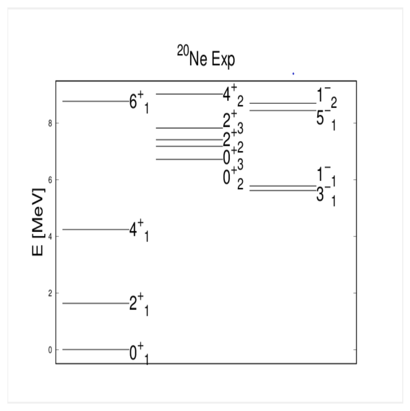
The model space is determined by the nuclear structure part and the number $n_{\pi }$ of the $\pi$- bosons. The minimal number of $n_{\pi }$ is zero. As long as true nuclear molecules are treated, as, e.g., the classical system ${}^{12}$C+${}^{12}$C [17], no serious problems arise, because the two clusters just touch and approximately can be treated independently, as noted in [1]. However, when the NVM is applied to the ground state and first excited states of a nucleus, as ${}^{20}$Ne →${}^{18}$O+$\alpha$ [18], the situation is quite different, because the overlap between the ${}^{16}$O and the $\alpha$ clusters is appreciable. The number of oscillation quanta of ${}^{20}$Ne, within the shell model, is 20 and the sum of oscillation quanta of oxygen and the $\alpha$ is just 12. Thus, as shown in [1,19,20] one needs minimally eight additional quanta. The corresponding $SU\left(3\right)$ irrep is (8,0) and reproduces the spectrum of ${}^{20}$Ne. Within the NVM the number of quanta starts from zero, i.e., the sequence of low lying $SU\left(3\right)$ irreps, containing positive parity states, is (0,0), (2,0), (4,0), etc. The angular momentum content is respectively [0], [0,2] and [0,2,4]. The negative parity states are contained in (1,0), (3,0), etc., with the angular momentum content [1] and [1,3] respectively. This is not the structure of the spectrum of ${}^{20}$Ne, whose experimental spectrum is shown in Figure 1.

A typical energy formula of the NVM is [15]

$$\begin{array}{ccc}\hfill E& =& {ϵ}_{\pi }{n}_{\pi }+\lambda n_{\pi }(n_{\pi }+3)+{\kappa }_1{\mathcal{C}}_2({\lambda }_a,{\mu }_a)+{\kappa }_2{\mathcal{C}}_2(\lambda ,\mu )+\xi L(L+1)\hfill \end{array}$$

(2)

The $n_{\pi }(n_{\pi }+3)$ is the eigenvalue of the second order Casimir operator of the relative motion. The expression ${\mathcal{C}}_2({\lambda }_a,{\mu }_a)$ denotes the eigenvalue of the second order Casimir operator of the structural part, the ${\mathcal{C}}_2(\lambda ,\mu )$ is the eigenvalue of the total relative motion $SU\left(3\right)$ irrep and the last term describes the rotational excitations. In (2) a great advantage of an algebraic model is seen: The algebraic model allows analytic formulas, at least in some limits, for a complicated nuclear system.

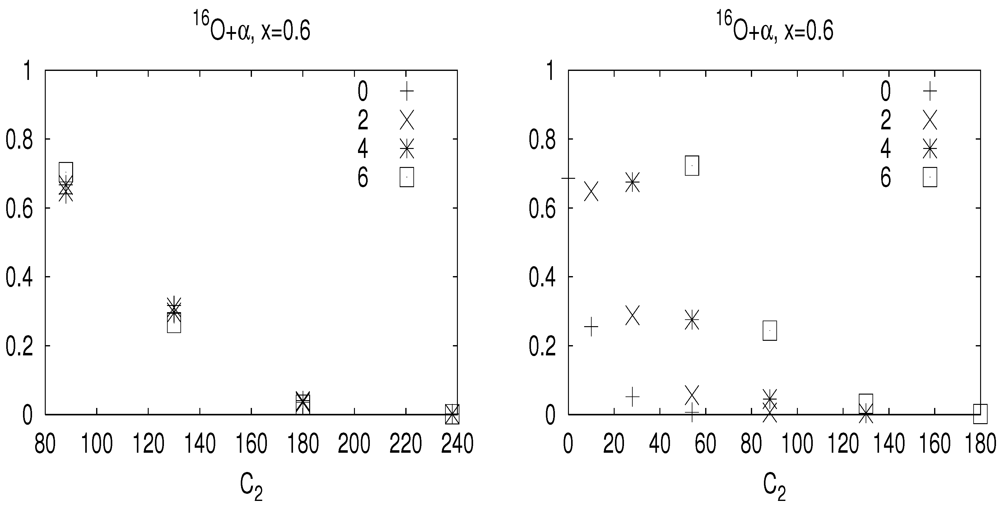
That there is a problem on how and where it is valid to apply the NVM was already exposed in [18], where the content of states in the same rotational band was compared to the NVM, see Figure 2. Rotational bands are characterized by the property that the intrinsic wave-function is at least approximately the same for all members in the same band (in particular there is always a mixing and one requires that the intrinsic state is similar for all members). In (8,0) all states have by construction the same structure, while it varies significantly passing from (0,0) to (2,0) and (4,0). The deformation is quite different between these irreps, see discussion in Section 3. Of course, an $L(L+1)$ rotational sequence can always be obtained by including a rotational term in the Hamiltonian. The difference between taking into account or not the PEP is illustrated in Figure 2 [18], for the cluster system ${}^{16}$O+$\alpha$. The vertical axis gives the contribution of different $SU\left(3\right)$-irreps to a particular state with spin L and the horizontal axis gives the eigenvalue of the second order Casimir operator with respect to this irrep. The left panel shows the case when the PEP is taking into account and, as can be seen, the content for states from $L=0$ up to $L=6$ is practically the same. This is not the case in the right panel, where the PEP is not taken into account.

The inclusion of the PEP also gives another interpretion of the vibrational limit $SU\left(3\right)$: as shown in [22], a minimal number of $\pi$-bosons implies a non-zero distance of the cluster in their ground state. Thus, the $SU\left(3\right)$ limit describes two clusters with a finite separation and the spectrum corresponds to a rotator, not a vibrator. What the inclusion of $SO\left(4\right)$ does is to increase this distance, i.e., making the system “more rigid”.

The NVM is thus the first example where a poorly planned application of an algebraic model can lead to an agreement to experimental data but the wrong states (they do not exist). The main reason is the use of a limited set of available data.

2.2. The Semimicroscopic Algebraic Cluster Model

A cluster model, used frequently by one of the authors, is the so-called Semimicroscopic Algebraic Cluster Model (SACM), introduced in [7,8].

For the sake of simplicity, we consider a two-cluster system: within the $SU\left(3\right)$ model of the nucleus [19,20] a light cluster can be characterized by the $SU\left(3\right)$-shell model quantum numbers $({\lambda }_k,{\mu }_k)$ ($k=1,2$). The two clusters are in their ground state. In addition, there is a relative motion, denoted by $(n_{\pi },0)$. This relative motion is generated by the basic degrees of freedom of $\pi$-bosons: ${\mathit{\pi }}_m^{†}$, ${\mathit{\pi }}^m$ ($m=-1,0,+1$). A cut-off is implemented, introducing an auxiliary scalar bosons ${\mathit{\sigma }}^{†}$, $\mathit{\sigma }$. This boson has no physical meaning, apart from introducing the cut-off. The cut-off is defined by the number N of total bosons, with

$$\begin{array}{ccc}\hfill N& =& n_{\pi }+n_{\sigma },\hfill \end{array}$$

(3)

where $n_{\pi }$ and $n_{\sigma }$ are the number of $\pi$- and $\sigma$-bosons, respectively. The number of $\pi$-bosons is limited from above by N, but also from below. This is the Wildermuth condition necessary for minimally observing the PEP. Usually, the minimal number $n_0$ of $\pi$-bosons is obtained by calculating the difference of the number of oscillation quanta in the united nucleus to the sum of oscillation quanta of the two clusters. For example, in ${}^{16}$O+$\alpha$→${}^{20}$Ne, the number of oscillation quanta in ${}^{16}$O is 12, in $\alpha$ it is zero and in ${}^{20}$Ne it is 20. Thus, the minimal number of $\pi$-bosons needed is $n_0$ = (20-12-0) = 8. Any smaller number implies to put a nucleon into an already occupied level, thus, violating the PEP. The above described method to obtain $n_0$ may fail when heavier nuclei are discussed. In this case one has to apply the concept of forbiddeness, introduced in [23] and put into a simple form in [24].

As shown in [7,8], the Wildermuth condition is necessary but not sufficient. In

$$\begin{array}{ccc}\hfill ({\lambda }_1,{\mu }_1)\otimes ({\lambda }_2,{\mu }_2)\otimes (n_{\pi },0)& =& \sum _{(\lambda ,\mu )}{m}_{(\lambda ,\mu )}(\lambda ,\mu ),\hfill \end{array}$$

(4)

where $m_{(\lambda ,\mu )}$ is the multiplicity of $(\lambda ,\mu )$ appearing in the product, the sum on the right contains still irreps of $SU\left(3\right)$, which do not observe the PEP. Therefore, this list is compared to the content of the shell model and only those irreps are retained which appear also in the shell model space. The states of a two-cluster system are denoted by the ket

$$\begin{array}{c}\hfill \mid N\left[({\lambda }_1,{\mu }_1),({\lambda }_2,{\mu }_2)\right]({\lambda }_C,{\mu }_C);(n_{\pi },0);(\lambda ,\mu ),\kappa LM\rangle ,\end{array}$$

(5)

where $({\lambda }_k,{\mu }_k)$ denote the $SU\left(3\right)$ irrep of the k’th cluster, which are coupled to $({\lambda }_C,{\mu }_C)$ and finally with the relative $SU\left(3\right)$ irrep $(n_{\pi },0)$ to the total irrep $(\lambda ,\mu )$. The $\kappa$ is a multiplicity index, L the angular momentum and M its magnetic projection.

In this manner, the model space of the SACM is microscopic. The part semi refers to the Hamiltonian used, which has the structure of a usual algebraic Hamiltonian, depending on a set of parameters (further below we will list a particular form of it).

The SACM is successfully applied to several cluster systems (see for example [25]) and further symmetry relations were found, as the multichannel symmetry [26]. In the multichannel symmetry the Hamiltonians of two or more clusterizations of the same united nucleus are related by some identical interaction terms, thus having the same parameters. This not only simplifies the application but in particular provides a profound relation between the clusters.

2.3. The Algebraic Cluster Model

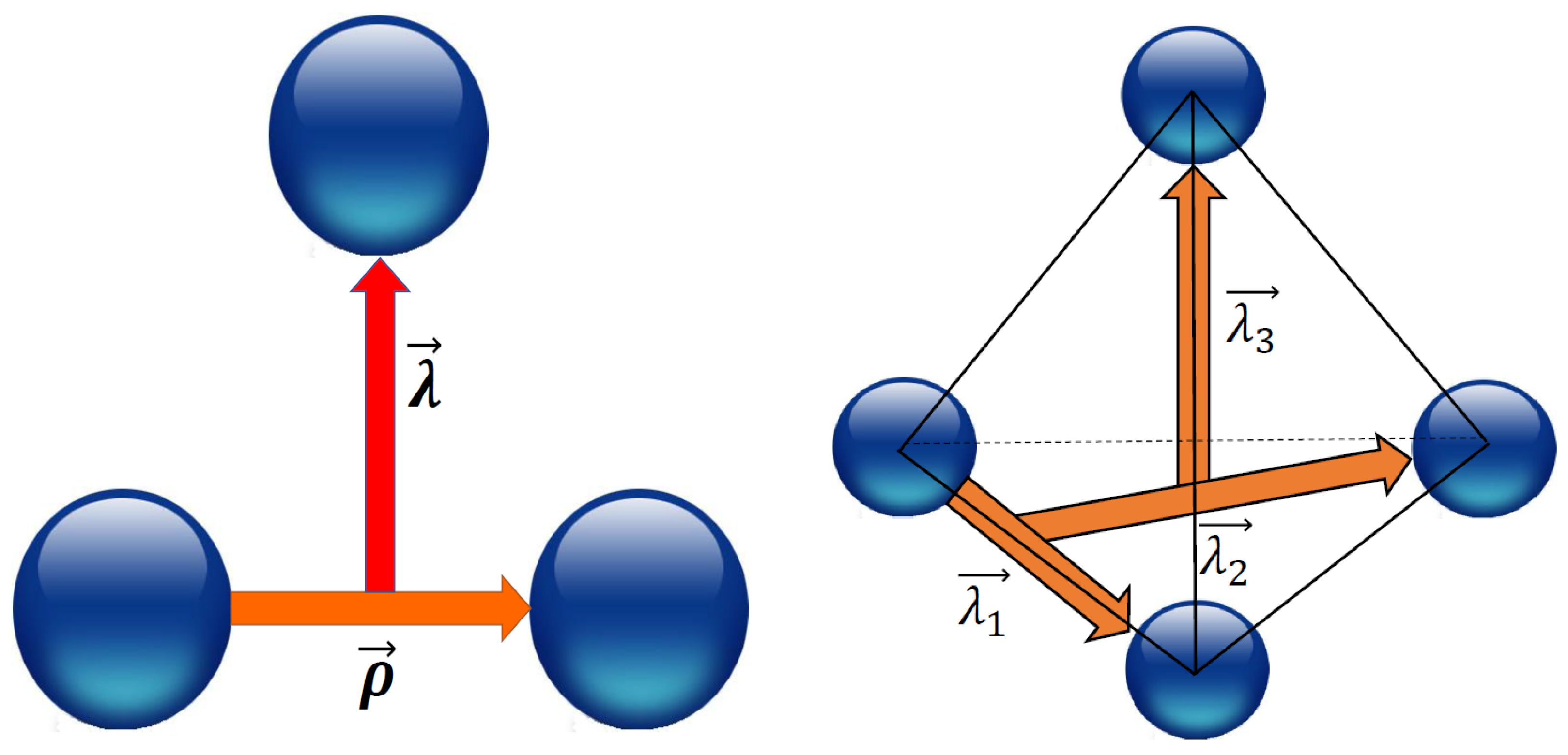
A first version of the Algebraic Cluster Model (ACM) was published in [27], in connection with a three-particle system. In [9] this model was applied to ${}^{12}$C and extended in [10] to ${}^{16}$O. In all these examples, the main mathematical tool is leaned from [11], which deals with atomic molecules, not nuclear cluster states. The ${}^{12}$C was supposed to be in a triangular and the ${}^{16}$O in a tetrahedral configuration. The multi-cluster system is excited by stretching and bending the assumed geometrical figure, apart from rotation. In Figure 3 the geometrical configuration of ${}^{12}$C and ${}^{16}$O is illustrated.

For example, the energy formula used in ${}^{12}$C is [9]

$$\begin{array}{ccc}\hfill E& =& E_0+{\omega }_1\left(v_1+\frac{1}{2}\right)\left(1-\frac{v_1+\frac{1}{2}}{N}\right){\omega }_2\left(v_2+1\right)\left(1-\frac{v_1+1}{N+\frac{1}{2}}\right)\hfill \\ & & +{\kappa }_{1}L(L+1)+{\kappa }_2{\left(K\mp 2l_2\right)}^2+\left[{\lambda }_1\left(v_1+\frac{1}{2}\right)+{\lambda }_2\left(v_2+1\right)\right]L(L+1).\hfill \end{array}$$

(6)

The quantum numbers are related to the representations of the group listed in [9] and are not of relevance here, except that (6) shows that simple energy formulas can be obtained. At first sight, the number of parameters seem to be 6 ($({\omega }_1,{\omega }_2,{\kappa }_1,{\kappa }_2),{\lambda }_1,{\lambda }_2)$, but in [9] the total number of bosons is also used as a parameter. This poses another problem: The N represents a cut-off and as such is not permitted to be used as a parameter in a consistent procedure.

For the ${}^{16}$O nucleus the following energy formula was used:

$$\begin{array}{ccc}\hfill E\left[v_1,v_2,v_3;\alpha ,L\right]& =& \frac{1}{2}{\omega }_1+\frac{1}{2}{\omega }_2+\frac{1}{2}{\omega }_3+B_{\left[v_1,v_2,v_3\right]\xi }L(L+1)\hfill \end{array}$$

(7)

where $\left[v_1,v_2,v_3\right]\alpha$ refers to a particular band and the $\left[v_1,v_2,v_3\right]\xi$ acquire the values $\left[000\right]A$, $\left[100\right]A$, $\left[010\right]E$, $\left[001\right]F$, the ${\omega }_k$ all have the same values of $6.05$ MeV. The $[v_1,v_2,v_3]$ refer to the quantum numbers of the vibrational modes [10]. The A, E and F denote different stretching modes.

This particular case fits quite well the experimental data, because it allows to fix by hand the band head and the moment of inertia within each band.

Furthermore, transition values and form factors were determined with a reasonable agreement to observation.

However, again, no PEP is observed. This will lead, as shown in the section of applications, to severe changes in the structure of the spectrum.

2.4. Applications to Multi-$Alpha$ Cluster Systems

Multi-$\alpha$ cluster systems enjoy a permanent interest due to their importance in Astophysics, i.e., the formation of elements in stars. For example, the ${}^{12}$C nucleus is produced in a triple-$\alpha$ process, possible due to existence of the Hoyle state [28], which is the aim of many studies in cluster physics, as is the case in the algebraic models discussed here.

Here, we will use as an example the structure of ${}^{12}$C as a three-$\alpha$ cluster system and ${}^{16}$O as a four-$\alpha$ cluster system. A review of recent advances of multi-$\alpha$ cluster studies is given in [29], based on microscopic approaches. In [29] a criterion is given, which tells the importance of the PEP: The antisymmetrization operator $\mathit{A}$ is applied on the state $\mid B\rangle$, where B is a parameter of this state. The criterion is that when

$$\begin{array}{ccc}\hfill N\left(B\right)& =& \frac{\langle B\mid \mathit{A}\mid B\rangle }{\langle B\mid B\rangle }\hfill \end{array}$$

(8)

$N\left(B\right)$ is small, the effect of the antisymmetrization is large, while when it tends to 1, the effect is small. In other words, when $N\left(B\right)$ is near to 1, the clusters can be treated as isolated. However, when $N\left(B\right)$ is small, the PEP has to be taken into account explicitly. For ${}^{12}$C the value of $N\left(B\right)$ is very small for the ground state (see Figure 10 in [29]), i.e., PEP cannot be neglected, and for the Hoyle state it is about 0.6, which indicates a still important influence of the PEP. The situation is similar for ${}^{16}$O. Only for $0^{+}$ states at large excitation energy the system can be treated approximately as a gas of $\alpha$-particles.

2.4.1. ${}^{12}$C

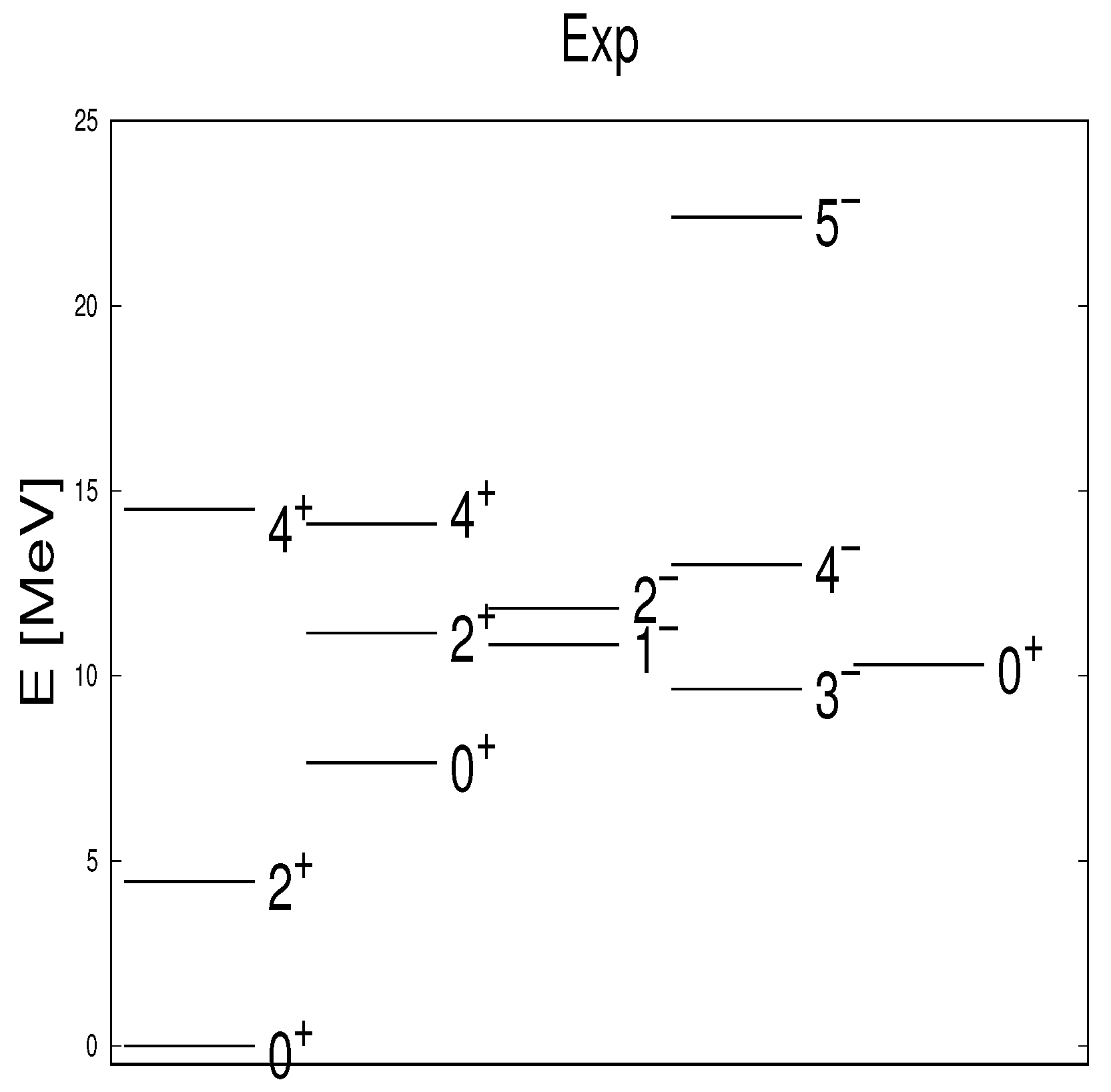
The experimentally known spectrum is depicted in Figure 4. The ACM and SACM will produce more states at low energy, thus the spectrum seems to be incomplete.

The model space within the SACM is constructed as follows:

• Each $\alpha$-cluster is assumed to be in a (0,0) irrep of the $SU\left(3\right)$ shell model.
• Between the first two $\alpha$’s the Wildermuth condition requires a minimal number of four oscillation quanta. (${}^8$Be has 4 oscillation quanta within the shell model and each $\alpha$ contributes zero, thus, 4 oscillation quanta have to be in the relative motion). The same is the case for the relative motion of the third $\alpha$ particle with respect to the first two. ${}^{12}$C has 8 oscillation quanta and the 2-$\alpha$ subsystem already 4, thus, 4 more oscillation quanta have to be added in the relative motion of the second Jacobi-coordinate.
• The symmetric states of the three $\alpha$-system is obtained using the procedure as exposes in [30].
• The obtained list of possible $SU\left(3\right)$ irreps is compared to the shell model space (programs are available for that), resulting in the final model space.

An alternative is to use the procedure proposed by the Anti-symmetric Molecular Dynamics theory (AMD) [5]. The procedure applied in the SACM and AMD lead to the same model space.

The model space is listed in

Table 1. The SACM Model space for the 3-$\alpha$ particle system, in agreement to [5,6]. The upper index indicates the multiplicity.

$\mathit{n}\mathit{\hslash }\mathit{\omega }$	$\left(\mathit{\lambda },\mathit{\mu }\right)$
0	(0,4)
1	(3,3)
2	(2,4), (6,2)
3	(3,4), (5,3), (9,1)
4	(0,6), (4,4), (6,3), (8,2), (12,0)
5	(3,5), (5,4), (7,3), (9,2), (11,1)
6	(2,6), (6,4)${}^2$, (8,3), (10,2), (12,1), (14,0)

, but some remarks on the geometrical interpretation of the multi-$\alpha$ partcile configuration are due: in the Algebraic Cluster Model (AIM) [9] it is emphasized that the distinct prediction is the triangular structure of the ${}^{12}$C. This is not a surprise. The three clusters are identical and therefore the distance of each of them to a second one has to be equal, no matter of the choice. The only geometrical configuration allowed is the triangular one. This is true for the ground state [22], but configuration mixing will blur the geometrical structure for higher lying states, as shown in microscopic calculations [31,32], where the Hoyle state tends to a linear chain. The situation is the same for ${}^{16}$O which has to be in a tetrahedral structure in its ground state, thus, we have already here a significant difference between the full microscopic treatment and the ACM. The geometrical structure for both nuclei, in terms of a multi-$\alpha$ cluster arrangement is illustrated by the cartoon in Figure 3. The consequences of symmetries in a 3-$\alpha$ particle system was also investigated in [33]. The results of the multichannel dynamical symmetry approach [26] was compared to the ACM. Using the available data, both models give similar results, as also for the SACM. The point is that more data are needed to show the clear difference in taking into account the PEP or not.

A second observation is that the PEP still plays an important role, in ${}^{12}$C and ${}^{16}$O, for the model space, see Table 1. There is no overlap of the intrinsic structure of the positive and negative parity states, opposed to the association of bands in the AIM. As shown in [34,35] the $SU\left(3\right)$ irrep $(\lambda ,\mu )$ satisfies a specific approximate quadrupole deformation formula, within the $SU\left(3\right)$ model:

$$\begin{array}{ccc}\hfill {\left({\beta }_2\right)}^2& =& \left(\frac{16\pi }{5N_0^2}\right)\left({\lambda }^2+{\mu }^2+\lambda \mu \right),\tan \gamma =\frac{\sqrt{3}\mu }{\left(\lambda +\mu \right)},\hfill \end{array}$$

(9)

where $N_0$ is the sum of all oscillation quanta plus $\frac{3}{2}(A-1)$, with A the number of nucleons. The ${\beta }_2$ is the quadrupole deformation and $\gamma$ describes the triaxiality [36].

The quadrupole deformation changes from irrep to irrep, i.e., different representations have a different quadrupole deformation, thus, belonging to different bands. For example, (0,4) has the deformation value 0.27 and the 1$\hslash \omega$excitation irrep (3,3) has the quadrupole deformation of 0.45.

The Hamiltonian is phenomenological, composed of a sum of physically motivated interactions:

$$\begin{array}{ccc}\hfill \mathit{H}& =& \hslash \omega {\mathit{n}}_{\pi }-\chi {\mathcal{C}}_2(\lambda ,\mu )+t_2{\left({\mathcal{C}}_2(\lambda ,\mu )\right)}^2+t{\mathcal{C}}_3(\lambda ,\mu )\hfill \\ & & +\left(a+a_L{(-1)}^L+a_{Lnp}\Delta {\mathit{n}}_{\pi }\right){\mathit{L}}^2+b{\mathit{K}}^2\hfill \\ & & +b_1\left[{\left({\mathit{\sigma }}^{†}\right)}^2-\left({\mathit{\pi }}^{†}·{\mathit{\pi }}^{†}\right)\right]·\left[h.c.\right].\hfill \end{array}$$

(10)

The First term sets the scale of the harmonic oscillator shell, i.e., $\hslash \omega =45A^{-\frac{1}{3}}-25A^{-\frac{2}{3}}$ and it is fixed [37] (A is the number of nucleons). The ${\mathcal{C}}_2(\lambda ,\mu )$ is the second order Casimir operator of $SU\left(3\right)$ and is proportional to the quadrupole-quadrupole interaction [34]. The ${\mathit{K}}^2$ term gives the square of the K-projection of the angular momentum onto the intrinsic z-axis and serves to distinguish states with the same angular momentum within a given $SU\left(3\right)$ irrep [38]. The $b_1$-term is proportional to a Casimir operator of $SO\left(4\right)$ and mixes $SU\left(3\right)$ irreps. The ${\mathit{L}}^2$ is the angular momentum operator with a factor simulating a variable moment of inertia. The remaining terms are corrections. The most general Hamiltonian of the SACM is not used here, keeping it simple for illustrative reasons.

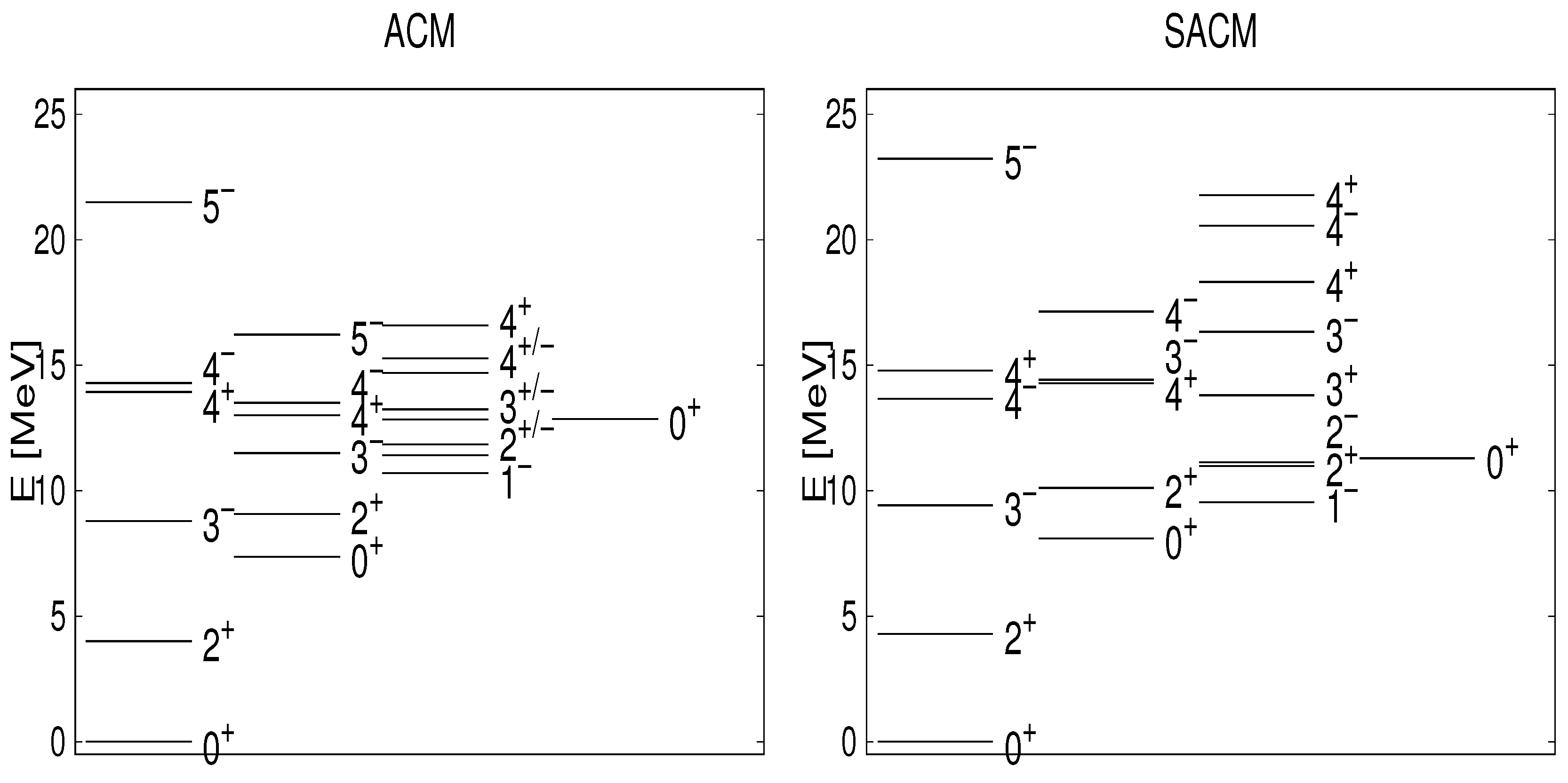
In Figure 5 the result of the ACM (left panel) and the SACM (right panel) are plotted. the spectrum obtained within the SACM and the ACM, respectively, are shown. The agreement to the the experimental known spectrum is quite well for both models (see [12,13]). However, comparing the ACM to the SACM, some differences are clearly visible.

• At low energy there is only one $5^{-}$ state in the SACM, while in the ACM there are 2, a consequence of ignoring the PEP.
• The spectrum in the ACM is denser at low energy than in the SACM. For example, several predicted parity doublets vanish when the PEP is taken into account.
• Within the ACM, the maximal number of bosons was used as a parameter, which is not allowed. The number N is a cut-off and convergence should be checked with increasing N. This is also a problem in the SACM: we used finite N, otherwise the space becomes too large. One conforms with a renormalization of the parameters when N increases.

The association into bands are completely different within the ACM and SACM. The ordering, as done in the ACM, is taken from atomic physics, while in SACM it is taken from the $SU\left(3\right)$ content of the shell model, which is clearly more appropriate.

As seen, though at first sight it seems that a model not taking into account the PEP leads to important structural changes, shedding some doubt on the ACM. Using methods from atomic molecules [11], is only partially valid.

In [12] $B\left(E2\right)$-values were also calculated and compared to the ACM and experiment. Due to the large deformation of ${}^{12}$C the mixing of the $SU\left(3\right)$ irreps become very important. The values obtained within the SACM are equally good as the ACM or even better (see

Table 2. Some calculated $B\left(E2\right)$ values of ${}^{12}$C, determined within the SACM and the ACM, compared to experimental available values. The numbers are in Weisskopf units (WU).

$\mathit{B}(\mathit{EL};{\mathit{J}}_{\mathit{i}}^{\mathit{\pi }}\to {\mathit{J}}_{\mathit{f}}^{\mathit{\pi }})$	EXP.[WU]	$\mathit{SU}\left(3\right)$ [WU]	SACM [WU]	ACM
$B(E2;2_1^{+}\to 0_1^{+})$	$4.65\pm 0.26$	4.65	5.37	5.15
$B(E2;0_2^{+}\to 2_1^{+})$	$8.\pm 0.11$	0.0	7.73	0.8
$B(E3;3_1^{-}\to 0_1^{+})$	$12.\pm 2$	6.32	24.28	5.14

). However, the main motivation in this contribution is not to get a pefect fit to the spectrum and $B\left(E2\right)$ values but rather demonstrate the importance of the PEP and what happens to the structure when the PEP is not considered.

2.4.2. ${}^{16}$O

The ${}^{16}$O was investigated within the ACM [10] and within the SACM in [13]. Within the SACM, the Hamiltonian was slightly different from the one in (10).

$$\begin{array}{ccc}\hfill \mathit{H}& =& \hslash \omega {\mathit{n}}_{\pi }-\chi \left(1-\xi \Delta {\mathit{n}}_{\pi }\right){\mathcal{C}}_2(\lambda ,\mu )+t_1{\mathcal{C}}_3(\lambda ,\mu )\hfill \\ & & +t_2{\left({\mathcal{C}}_2(\lambda ,\mu )\right)}^2+\left(a+a_{Lnp}\Delta {\mathit{n}}_{\pi }\right){\mathit{L}}^2+b{\mathit{K}}^2\hfill \\ & & +b_1\left[{\left({\mathit{\sigma }}^{†}\right)}^2-\left({\mathit{\pi }}^{†}·{\mathit{\pi }}^{†}\right)\right]·\left[h.c.\right].\hfill \end{array}$$

(11)

It is, as for ${}^{12}$C, a function of Casimir operators. The last line is responsible for the mixing of $SU\left(3\right)$ irreps, while the first terms are completely within the $SU\left(3\right)$ limit and, alone, permit an analytic solution.

Within the SACM, the space was obtained by first constructing all states, symmetric under permutations of the $\alpha$-particles, using the path shown in [30,39]. The obtained list of $(\lambda ,\mu )$ irreps is compared to the shell model. The final result is depicted on the right hand side of

Table 3. The model space of the 4-$\alpha$ partcile system, according to [6] (left panel) and the SACM (right panel). The $SU\left(3\right)$ irrep in italic (left side) does not appear in the model space of the SACM, as the irreps in italic on the right side do not appear in the list given in [6]. In addition, some multiplicities of irrep in the SACM are larger than in [6]. We show only the irreps up to 4 excitation quanta, otherwise the table would get quite dense. Differences between the two lists appear from 3$\hslash \omega$ shell excitations on.

$\mathit{n}\mathit{\hslash }\mathit{\omega }$	Kato	SACM
0	$(0,0)$	$(0,0)$
1	$(2,1)$	$(2,1)$
2	$(2,0)(3,1)(0,4)(4,2)$	$(2,0)(3,1)(0,4)(4,2)$
3	$(3,0)(0,3)(2,2)(4,1)(3,3)(6,0)\left(5.2\right)(2,5)(6,3)$	$(3,0)(0,3)(2,2)(4,1)(1,4)(3,3)(6,0)(5,2)(2,5)(6,3)$
4	$(0,2)(1,3){(4,0)}^2(3,2){(2,4)}^2{(5,1)}^2(4,3)$	$(0,2)(2,1){(1,3)}^2{(4,0)}^2{(3,2)}^2{(2,4)}^4{(5,1)}^3{(4,3)}^2(1,6)$
	$(3,5){(6,2)}^2(5,4)(0,8)(8,1)(4,6)(7,3)(8,4)$	${(3,5)}^2{(6,2)}^3(5,4)(0,8)(4,6)(7,3)(8,4)$

, compared to the result obtained by [6] using an explicit approach to determine the anti-symmetrized states. As noted, in this 4-$\alpha$-particle system the SACM has more states than given by [6]. The difference consists in a larger multiplicity than the ones listed by [6]. In addition, there appear some states in the SACM which do not appear in [6]. In a few occasions, there are irreps in [6] which do not appear in the SACM. Note, for small excitation quanta the two lists coincide and the differences start at 3$\hslash \omega$ shell excitations.

Fortunately, the additional states are at high energy, so when the calculation of the spectrum is performed, these states do not show up at low energy and have little influence on the structure of the low lying states (please, consult Figure 6). Nevertheless, this shows that also the SACM has a component of violating the PEP. Such differences do not appear for a two-cluster system, to our knowledge. Probably they are the result of increasing the number of clusters. In case of ${}^{16}$O, the states are by construction symmetric under the permutations of the $\alpha$-particles [30,39]. This leads us to the comparison of the list of symmetric states to the shell model space. Though an irrep appears in the shell model space and in the list of symmetrized $\alpha$-particle space, the corresponding state in the shell model space does probably not correspond to a symmetrized 4$\alpha$ particle state. How to solve this and on how to identify the non-symmetric states in the shell model space, is still under investigation by us. Nevertheless, due to the exclusion of most non-allowed states, the SACM is still better suited as an algebraic model than the ACM.

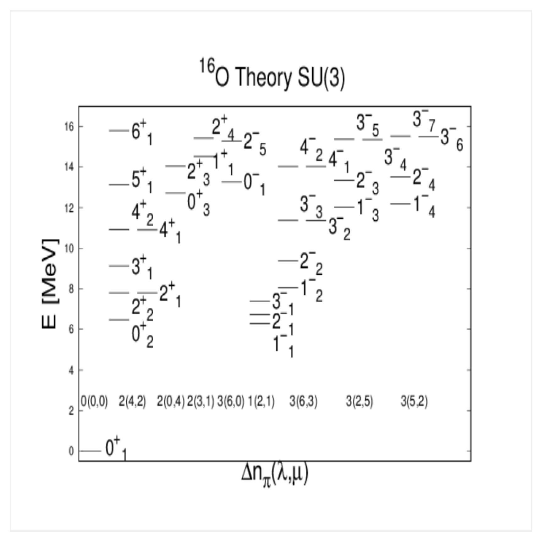
The ${}^{16}$O nucleus is a perfect example of a $SU\left(3\right)$ nucleus. The deformation in its ground state is zero and the mixing to other $SU\left(3\right)$ irreps is negligible. In fact, the ground state consists only of one, namely the $0^{+}$ state.

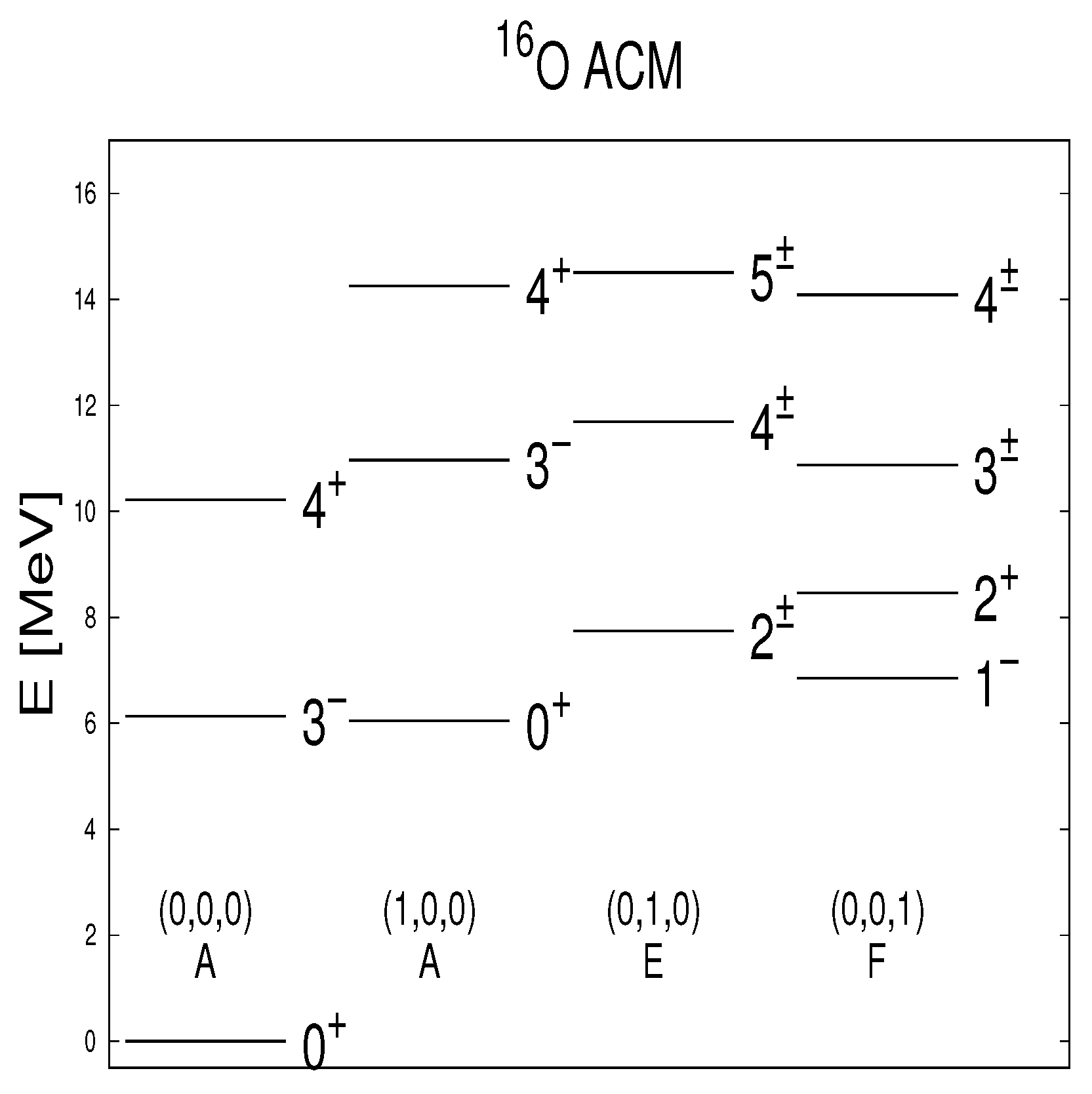
This is in contrast to the ACM, where the ground state band consists of many levels (0${}^{+}$, $3^{-}$ and 4${}^{+}$), ordered in a band of mixed positive and negative parity states, see Figure 6 for the SACM compared to Figure 7 for the ACM. The agreement to the experimentally known states is good in both models. Nevertheless, as in ${}^{12}$C, the larger density of the states in the ACM is the effect of not observing the PEP and the picture obtained is flawed. One reason is that the experimental data used is limited, i.e., not complete.

Furthermore the claim by the ACM, that ACM predicts a tetrahedral structure is not restricted to the ACM, because ${}^{16}$O has to be tetrahedral, which can also be shown, using the geometrical mapping according to [22]. As mentioned already further above, the argument is even simpler, noting that the $\alpha$-particles have to be symmetric under permutations, i.e., the distance of one to any other particle has to be the same. This is only achieved by the tetrahedral structure, in its ground state. This interpretation in terms of a tetrahedral structure does not take into account one important effect: The one of antisymmetrizing a state. This antisymmetrization erases in ${}^{16}$O the memory of a tetrahedral structure and produces a perfectly spherical nucleus, also in its intrinsic reference frame. Sometimes, as in ${}^8$Be the visible structure in terms of two $\alpha$ particles is apparently maintained, but also this can lead to erroneous interpretations. What is obtained is a density distribution, which only shows an explicit separation into two blobs, summed over each corresponds to the content equivalent to an $\alpha$-particle, but the nucleons of ${}^8$Be are still distributed over the whole nucleus.

A conclusion of this section is that the PEP is important and it cannot be neglected. Any attempt to avoid the PEP leads to erroneous interpretations. Furthermore, algebraic models, with the right amount of parameters, are effective to adjust the theoretical spectrum to a limited list of available experimental states. This is due to the problem that not all states at low energy are known. Therefore, it is important for the future to measure the full spectrum of ${}^{12}$C and ${}^{16}$O in order to give a nice lesson on how to interpret an algebraic model.

3. Algebraic Models in Nuclear Structure Physics

Algebraic models have a long tradition in nuclear structure physics. In [19,20] J. P. Elliott introduced the the $SU\left(3\right)$ model for deformed sd-shell nuclei, proving that an algebraic model can explain the spectrum of deformed nuclei, practically impossible within shell model calculations at that time. In the 70’s F. Iachello proposed the IBM [14] which provides a complete and elegant description of the collective quadrupole structure. Since then the IBM has been extended to many different versions and showed the power of algebraic method.

Here, we will consider the IBM as an example and that it is essential to take into account all the basic assumptions of the model.

The Interacting Boson Model

The Interaction Boson Model (IBM) [14] is one of the most successful models in nuclear structure. It is the basis for extensions, as to odd–even, even–odd and odd–odd nucleus [40]. Using a super-symmetric extension to groups of even–even, even–odd, odd–even and odd–odd nuclei, one was able to prove that in nuclear physics systems a kind of super-symmetry exist [41], not yet encountered in particle physics.

However, let us concentrate on the IBM version, applied to even–even nuclei only. All other extensions have similar characteristics and problems.

Before doing so, we will briefly resume the main steps of an algebraic model, as the ones in the last section, in order to make a point. Though, at first sight, to many it will appear trivial in what follows, the devil lies in the details on how to interpret the physics and the path taken. Knowing the basic degrees of freedom is important but not taking into account basic assumptions and structures of the physical system in consideration, can lead to an inconsistent interpretation of the physics involved and may in fact lead to a different kind of model. The other, mathematical equivalent (see also [42]), model may work well and thus also the algebraic model, one starts with, has to reproduce the spectrum and transition values.

We will make a detour in order to emphasize a delicate point, considered usually as trivial: We will construct a model on pure mathematical grounds, not related to physics. The point to make is that the physics could in principle be ignored, but it should not.

In general, the number of degrees of freedom n of a system have to be identified. For the moment, it does not matter what these degrees of freedom are. Furthermore, for simplicity, we restrict to bosonic degrees of freedom. For fermionic degrees of freedom the arguments are identical. Let us denote by ${\mathit{b}}_i^{†}$ and ${\mathit{b}}^i$ the boson creation and annihilation operators. The position of the index indicates the different transformation properties: while ${\mathit{b}}_i^{†}$ transforms co-variant, the ${\mathit{b}}^i$ transforms contra-variant. This notation is easier to handle than the one usually used (tilde- and star-operations). The indices $i,j$ range from 1 to n.

The following operators are defined

$$\begin{array}{ccc}\hfill {\mathit{C}}_i^j& =& {\mathit{b}}_i^{†}{\mathit{b}}^i,\hfill \end{array}$$

(12)

which form the algebra of $U\left(n\right)$:

$$\begin{array}{ccc}\hfill \left[{\mathit{C}}_i^j,{\mathit{C}}_p^q\right]& =& {\delta }_{jp}{\mathit{C}}_i^q-{\delta }_{iq}{\mathit{C}}_p^j.\hfill \end{array}$$

(13)

This notation is also useful for the construction of Casimir operators, those which commute with all generators: The Casimir operator of order m is given by

$$\begin{array}{ccc}\hfill {\mathcal{C}}_m& =& \sum _{i_1,\dots ,i_m}{\mathit{C}}_{i_1}^{i_2}{\mathit{C}}_{i_2}^{i_3}\dots {\mathit{C}}_{i_m}^{i_1},\hfill \end{array}$$

(14)

For example, the first order Casimir operator is ${\mathcal{C}}_1={\sum }_i{\mathit{C}}_i^i$, i.e., just the number operator.

Going from $U\left(n\right)$ to $SU\left(n\right)$ is done by redefining the $U\left(n\right)$ operators as

$$\begin{array}{ccc}\hfill {\mathit{C}}_i^j& \to & {\mathit{C}}_i^j-\frac{{\delta }_{ij}}{n}\sum _k{\mathit{C}}_k^k.\hfill \end{array}$$

(15)

The algebra of these operators is the one of $SU\left(n\right)$ and is similar to the one of $U\left(n\right)$.

The next step is to look for subgroup chains of the type

$$\begin{array}{cc}\hfill U\left(n\right)& \supset G_1\supset G_2\supset \dots .\supset SO\left(3\right)\\ \hfill U\left(n\right)& \supset G_1^{\prime }\supset G_2^{\prime }\supset \dots .\supset SO\left(3\right)\\ & \dots \dots \dots \dots \dots \dots \dots ..& ,\hfill \end{array}$$

(16)

where, with nuclear physics in mind, each chain ends in the $SO\left(3\right)$, the angular momentum group. In particle physics it would be the $U\left(1\right)\wedge SU\left(2\right)$ group, with ∧ denoting a semi-direct product. In general, there exist more than one chain of groups (denoted symbolically by the other chain), each representing a different internal structure and correspond to different dynamical symmetries. There might be more than one group chain for different dynamical symmetry limits, indicated by the dotted line.

This procedure does not depend on the type of degrees of freedom. However, it is a very useful path to introduce some systematic order to the system.

Once you have obtained this mathematical result, one proceeds to define algebraic Hamiltonians, that satisfy the condition to preserve the number of bosons. One possibility is to use a sum of functions, depending each on Casimir operators of the same chain (16). For example, using the first chain in (16), a possible Hamiltonian is

$$\begin{array}{ccc}\hfill \mathit{H}& =& \omega \mathit{N}+{\chi }_1{\mathcal{C}}_{G_1}+{\chi }_2{\mathcal{C}}_{G_2}+\dots +\xi {\mathit{L}}^2,\hfill \end{array}$$

(17)

where N is the number operator of $U\left(n\right)$, ${\mathcal{C}}_{G_k}$ a Casimir operator of the group $G_k$ and ${\mathit{L}}^2$ the angular momentum operator, though in our example it is just the Casimir operator of a $SO\left(3\right)$ group.

Equation (17) permits the analytical solution

$$\begin{array}{ccc}\hfill E& =& \omega N+{\chi }_1{c}_{G_1}+{\chi }_2{c}_{G_2}+\dots +\xi L(L+1),\hfill \end{array}$$

(18)

with $c_{G_k}$ as the eigenvalue of the ${\mathcal{C}}_{G_1}$ Casimir operator.

This property, that the Hamiltonian is a function in the Casimir operator of one chain and permits an analytical solution, is called a dynamical symmetry [43].

The advantage is that this Hamiltonian is by construction diagonal in the basis defined by one of the chains (16). In general, all possible Casimir operators of all appearing chains of groups of the type (16) can be used. Note, a Casimir operator in one dynamical symmetry chain does not commute with a Casimir operator from another dynamical symmetry chain. In this case, no analytic results can be given, but the group theory allows to calculate matrix elements, which provides us with the possibility to diagonalize the Hamiltonian.

To resume what has been presented up to now, taking any number of degrees of freedom, one can construct states and Hamiltonians with analytic solutions, without having specified yet which physical system is treated. This yet missing part of physics is included by identifying the physical system and using its properties, e.g., if the bosons are exact, which are the number of basic degrees of freedom of the bosons involved, if the bosons have sub-structure or not, etc.

Up to now we have not specified the physical system under consideration. This might present a problem: when two different models, applied to the same physical system, presenting each the same number of basic degrees of freedom, mathematically they are indistinguishable, except when the differences between them is exploited, for example, the differences in the model space and the Hamiltonian.

In case of nuclear physics, the IBM proposes to group the nucleon pairs in the valence shells to bosons with angular momentum zero (scalar bosons ${\mathit{s}}^{†}$, s) and of angular momentum 2 (${\mathit{d}}_m^{†}$, ${\mathit{d}}^m$ ($m=-2,-1,0,+1,+2$). In total there are six degrees of freedom and, thus, a $U\left(6\right)$ appears.

There exist three group chains, starting from $U\left(6\right)$, which contain the $SO\left(3\right)$ group:

$$\begin{array}{ccc}\hfill U\left(6\right)& \supset U\left(5\right)\supset & SO\left(3\right)\hfill \\ \hfill U\left(6\right)& \supset SU\left(3\right)\supset & SO\left(3\right)\hfill \\ \hfill U\left(6\right)& \supset O\left(6\right)\supset & SO\left(3\right).\hfill \end{array}$$

(19)

The first chain is called the vibrational limit. The $U\left(5\right)$ subgroup is obtained by just skipping the scalar boson, i.e., there are five degrees of freedom left. The second chain is called the rotational limit and the third chain the $\gamma$-unstable limit. This notation is due to the type of spectrum which arises and the type of semi-classical potential, obtained in a geometrical mapping [44].

The IBM is able to reproduce a large variety of nuclei with such a simple but effective model.

One of the main assumptions of the IBM is that pairs of nucleons can be mapped to bosons. How to do it in a consistent manner is published in [45]. A necessary condition is that the total number of bosons is half the number of valence nucleons.

As an example, we use a possible Hamiltonian in the $SU\left(3\right)$ limit and its analytical eigenvalue. The states are classified according to the collection of quantum numbers, denoted by the ket

$$\begin{array}{c}\hfill \mid N(\lambda ,\mu )\kappa LM\rangle ,\end{array}$$

(20)

where N is the total number of bosons, $(\lambda ,\mu )$ denotes the $SU\left(3\right)$ irrep, L is the angular momentum, M its projection and $\kappa$ is a multiplicity index. Note, that there is no need to use the number of s- (monopole) and d- (quadrupole) bosons, because they are mixed.

The example Hamiltonian is

$$\begin{array}{ccc}\hfill \mathit{H}& =& {ϵ}_d{\mathit{n}}_d-\chi {\mathcal{C}}_2(\lambda ,\mu )+\xi {\mathit{L}}^2,\hfill \end{array}$$

(21)

where ${\mathit{n}}_d$ is the number of d-bosons, ${\mathcal{C}}_2(\lambda ,\mu )$ the second order Casimir operator of $SU\left(3\right)$ and ${\mathit{L}}^2$ the angular momentum operator. The eigenvalue of (21) is

$$\begin{array}{ccc}\hfill E& =& {ϵ}_d{n}_d-\chi ({\lambda }^2+\lambda \mu +{\mu }^2+3\lambda +3\mu )+\xi L(L+1).\hfill \end{array}$$

(22)

Up to here, everything seems to be fine. Problems arise when situations are acquired where it is important to take into account the substructure of the bosons. This is the case in the mid-shell nuclei within the shell model, i.e., just where the $SU\left(3\right)$ limit should work. The exact boson mapping as given in [45], leads to higher order terms in the Hamiltonian. However, not only that, the change in the model space has to be taken into account, too. Unfortunately, this is not done in the IBM, which remains with the pure bosons. In [46] this problem is mentioned as the fatal flaw of the IBM, though we do not agree with the notion of fatal, because the model works and only needs a new interpretation.

The IBM shifts to a model which has six degrees of freedom and whose number of bosons are cut-off from above. Let us now compare the IBM with another model with the same degrees of freedom, namely the geometric model of the nucleus [36], which describes excitations as quadrupole changes in the surface of a nucleus. The basic degrees of freedom are the five quadrupole coordinates ${\alpha }_{2m}$ and the correponding boson creation and annihilation operators. What is not done in the original work, but can be done, is to introduce an auxiliary scalar boson $\sigma$ and demanding that the total number of quadrupole and scalar bosons is fixed. This was already mentioned in [42], relating the degrees of freedom of geometrical model (including the scalar boson) to the IBM approach. In [47] the geometrical model was reformulated in terms of d-bosons, with a complicated structure of the Hamiltonian, due to the contribution of the boson mapping excluding the explicit expression in terms of s-bosons, otherwise the model is equivalent to the IBM. This relation was also investigated in [48], where the mathematical equivalence between the IBA and the geometric model was demonstrated. Thus, the geometric model has the same degrees of freedom as the IBM. The difference is that while the IBM is limited to a fixed number of bosons the maximal number of bosons in the geometrical model has to be increased until convergence of the results at low energy is achieved. Ignoring the PEP, the IBM is transformed to the geometrical model of the nucleus with a finite cut-off. This difference has to be exploited when both models are compared.

So, how to distinguish between them? One way is to take into account the change in the model space, as discussed in [49,50]. There it is shown that for mid-shell nuclei the sequence of $SU\left(3\right)$ irreps do not start from (2N,0) and (2N-4,2), but with $(\lambda ,\mu )$ irreps with both numbers $\lambda$ and $\mu$ different from zero. This has an important consequence: the (2N,0) has the sequence $0^{+}$, $2^{+}$, etc., the $(2N-2,2)$ contains a $\gamma$-band starting with a $2^{+}$ state. While in the first choice of irreps there are no $B\left(E2\right)$ transitions between the $\gamma$-band and the ground state (they belong to different $SU\left(3\right)$ irreps and the quadrupole operator, a $SU\left(3\right)$ generator, cannot connect different irreps), in the second choice there are transitions. Instead of taking into account the remark by K. T. Hecht [49,50] one rather prefers to introduce the g-bosons and more parameters in order to resolve this problem [51].

Taking into account the arguments above, the IBM transforms to a model equivalent to the geometrical one with a cut-off. Can this be used to discriminate between the geometrical model and the IBM? Rather not. In [52] the ${}^{196}$Pt was compared to the geometric model [53] and the IBM (see the report [54] and references therein). The conclusion was that the geometrical model fits better the data and the reason is the cut-off in the IBM, as concluded in [52]. However, this is just one case. Another example is the application to ${}^{168}$Er. In [55] the IBM was applied to this nucleus with a very complicated spectrum and the agreement is excellent. Comparison to a simple geometrical model did not work well. However, in [56] it was criticized that the version of the geometrical model used in [55] was not valid and an application to the general geometrical model [57] yielded no difference. The reason for the agreement of both models is that in the IBM the number of bosons is sufficiently large.

Nevertheless, with the help of the IBM a more powerful description of the nuclear structure is possible. The extensions to odd–even, even–odd and odd–odd nuclei is easier to realize, not as proposed in the geometric model [36]. Again, showing the power which lies within the use of an algebraic approach to nuclear structure, but also that ignoring the PEP leads to a flawed physical interpretation of collective nuclear states.

There are several efforts to relate the IBM to the shell model, see for example [42,58]. In [42] correlated D- and S-fermion pairs were mapped to the d- and s-bosons. Starting from a microscopic model Hamiltonian, the IBM Hamiltonian is obtained. Matrix elements of the physical operators, as interaction terms and transition operators, are compared to their microscopic counter parts, yielding a mapping of the interaction parameters in the microscopic model to their IBM counterparts. In this way a mapping of a microscopic model to the IBM was achieved at the beginning of the shell, where the method is easy to apply and where also the boson approximation is valid due to the small overlap of these bosons. Approaching the mid-shell, however, problems with the PEP appears and the resolution of it is transferred to future studies.

4. Conclusions

We have presented an investigation on the importance of the Pauli Exclusion Principle (PEP) in nuclear structure physics, as models on nuclear clusters and structure models of the quadrupole degree of freedom.

In case of the cluster models we showed that not including the PEP leads to misinterpretations of bands and obscures rather the physis. We discussed in particular the systems of ${}^{12}$C and ${}^{16}$O and treated them with in the Semimicroscopic Algebraic Cluster model (SACM) and with in the Algebraic Cluster Model (ACM). While the SACM treats the PEP, it is avoided within the ACM. Both models seem to reproduce the experiment, which is due to too the limited number of experimentally known states and transitions. The structure of the states, however, are completely different and proves the importance of the PEP. In a multi-cluster system the SACM seems to have also a problem with the PEP, containing more $SU\left(3\right)$ irreps for a given number of shell excitations than in the Antizymmetrized Molecular Dynamics (AMD). Fortunately, these states appear at higher shell excitations and do not or little (in case of mixing) contribute to the structure of states at low energy. Therefore, it is still better than the ACM.

In the second part we investigated the importance of the PEP in the algebraic model for the quadrupole modes, called the Interacting Boson Model (IBM). It works, however, only due to a common misunderstanding of algebraic method used: starting with the known degrees of freedom, which determines the symmetry group, one continues with the standard methods to construct Hamiltonians and transition operators and forgets about some basic assumptions of the model, though it is claimed not to do so. In case of the IBM, the finite number of bosons enters in the total number of d- and s-bosons, but in no way the internal structure of the bosons is taken into account. This leads for mid-shell nuclei to a faulty interpretation. The reason why the Interacting Boson Approximation (IBA) works lies in the existence of another, geometrical model with the same degrees of freedom., i.e., this ambiguity appears always when two models exist with the same degrees of freedom. We proposed how the difference between the models should be exploited.

We hope that this contribution serves also as a warning and clarifies on how to and when the PEP has to be included.

References

- Wildermuth, K.; Tang, Y.C. A Unified Theory of the Nucleus; Academic Press: New York, NY, USA, 1977. [Google Scholar]
- Greiner, W.; Park, J.Y.; Scheid, W. Nuclear Moledcules; World Scientific: Singapore, 1995. [Google Scholar]
- Tohsaki, A.; Horiuchi, H.; Schuck, P.; Röpke, G. Alpha Cluster Condensation in 12C and 16O. Phys. Rev. Lett. 2001, 87, 192501. [Google Scholar] [CrossRef] [Green Version]
- Dreyfuss, A.C.; Launey, K.D.; Dytrych, T.; Draayer, J.P.; Bahri, C. Hoyle state and rotational features in Carbon-12 within a no-core shell-model framework. Phys. Lett. B 2013, 727, 511. [Google Scholar] [CrossRef] [Green Version]
- Horiuchi, H. Three-Alpha Model of 12C. Prog. Theor. Phys. 1974, 51, 1266. [Google Scholar] [CrossRef] [Green Version]
- Katō, K.; Fukatsu, K.; Tanaka, H. Systematic Construction Method of Multi-Cluster Pauli-Allowed States. Prog. Theor. Phys. 1988, 80, 663. [Google Scholar] [CrossRef]
- Cseh, J. Semimicroscopic algebraic description of nuclear cluster states. Vibron model coupled to the SU(3) shell model. Phys. Lett. B 1992, 281, 173. [Google Scholar] [CrossRef]
- Cseh, J.; Lévai, G. Semimicroscopic Algebraic Cluster Model of Light Nuclei. I. Two-Cluster-Systems with Spin-Isospin-Free Interactions. Ann. Phys. (N. Y.) 1994, 230, 165. [Google Scholar] [CrossRef]
- Marin-Lambarri, D.J.; Bijker, R.; Freer, M.; Gai, M.; Kokalova, T.; Parker, D.J.; Wheldon, C. Evidence for Triangular D3h Symmetry in 12C. Phys. Rev. lett. 2014, 113, 012502. [Google Scholar] [CrossRef] [Green Version]
- Bijker, R.; Iachello, F. The algebraic cluster model: Structure of 16O. Nucl. Phys. A 2017, 957, 154. [Google Scholar] [CrossRef] [Green Version]
- Herzberg, G. Molecular Spectra and Molecular Structure; D. Van Nostrand Company INC.: New York, NY, USA, 1963. [Google Scholar]
- Hess, P.O. 12C within the Semimicroscopic Algebraic Cluster Model. Eur. Phys. J. A 2018, 54, 32. [Google Scholar] [CrossRef]
- Hess, P.O.; Berriel-Aguayo, J.R.; Chávez-Nuñez, L.J. 16O within the Semimicroscopic Algebraic Cluster Model and the importance of the Pauli Exclusion Principle. Eur. Phys. J. A 2019, 55, 71. [Google Scholar] [CrossRef] [Green Version]
- Arima, A.; Iachello, F. The Interacting Boson Model; Cambridge University Press: Cambridge, UK, 1987. [Google Scholar]
- Daley, H.J.; Iachello, F. Nuclear vibron model. I. The SU(3) limit. Ann. Phys. 1986, 167, 73. [Google Scholar] [CrossRef]
- López-Moreno, E.; Castaños, O. Shapes and stability within the interacting boson model: Dynamical symmetries. Phys. Rev. C 1996, 54, 2374. [Google Scholar] [CrossRef] [PubMed]
- Bromley, D.A.; Kuehner, J.A.; Almqvist, E. Resonant Elastic Scattering of C12 by Carbon. Phys. Rev. Lett. 1960, 4, 365. [Google Scholar] [CrossRef]
- Yépez-Martínez, H.; Cseh, J.; Hess, P.O. Phase transitions in algebraic cluster models. Phys. Rev. C 2006, 74, 024319. [Google Scholar] [CrossRef]
- Elliott, J.P. Collective motion in the nuclear shell model. I. Classification schemes for states of mixed configurations. Proc. R. Soc. Lond. A 1958, 245, 128. [Google Scholar]
- Elliott, J.P. Collective motion in the nuclear shell model II. The introduction of intrinsic wave-functions. Proc. R. Soc. London A 1958, 245, 562. [Google Scholar]
- Available online: www.nndc.bnl.gov/ensdf (accessed on 12 April 2020).
- Hess, P.O.; Lévai, G.; Cseh, J. Geometrical interpretation of the semimicroscopic algebraic cluster model. Phys. Rev. C 1996, 54, 2345. [Google Scholar] [CrossRef]
- Smirnov, Y.F.; Tchuvil’sky, Y.M. The structural forbiddenness of the heavy fragmentation of the atomic nucleus. Phys. Lett. B 1984, 134, 25. [Google Scholar] [CrossRef]
- Yépez-Martínez, H.; Hess, P.O. The concept of nuclear cluster forbiddenness. J. Phys. G 2015, 42, 095109. [Google Scholar]
- Yépez-Martínez, H.; Ermamatov, M.J.; Fraser, P.R.; Hess, P.O. Application of the semimicroscopic algebraic cluster model to core+α nuclei in the p and sd shells. Phys. Rev. C 2012, 86, 034309. [Google Scholar]
- Cseh, J. Multichannel dynamical symmetry and heavy ion resonances J. Cseh. Phys. Rev. C 1994, 50, 2240. [Google Scholar] [CrossRef]
- Bijker, R.; Iachello, F. The Algebraic Cluster Model: Three-Body Clusters. Ann. Phys. (N. Y.) 2002, 298, 334. [Google Scholar] [CrossRef] [Green Version]
- Hoyle, F. On Nuclear Reactions Occuring in Very Hot STARS.I. the Synthesis of Elements from Carbon to Nickel. Astrophys. J. Suppl. 1954, 1, 121. [Google Scholar] [CrossRef]
- Schuck, P.; Funaki, Y.; Horiuchi, H.; Röpke, G.R.; Tohsaki, A.; Yamadas, T. Alpha particle clusters and their condensation in nuclear systems. Phys. Scr. 2016, 91, 123001. [Google Scholar] [CrossRef]
- Moshinsky, M.; Smirnov, Y.F. The Harmonic Oscillator in Modern Physics; Harwood Academic Publishers: New York, NY, USA, 1996. [Google Scholar]
- Kanada-En’yo, Y. The Structure of Ground and Excited States of 12C. Prog. Theor. Phys. 2007, 117, 655. [Google Scholar] [CrossRef]
- Chernykh, M.; Feldmeier, H.; Neff, T. Structure of the Hoyle State in 12C. Phys. Rev. Lett. 2007, 98, 032501. [Google Scholar] [CrossRef]
- Cseh, J.; Trencsényi, R. On the symmetries of the 12C nucleus. Int. J. Mod. Phys. E 2018, 27, 1850013. [Google Scholar] [CrossRef]
- Castaños, O.; Draayer, J.P.; Leschber, Y. Shape variables and the sehll model. Zeitschr. f. Physik A 1988, 329, 33. [Google Scholar]
- Rowe, D.J. Microscopic theory of the nuclear collective model. Rep. Prog. Phys. 1985, 48, 1419. [Google Scholar] [CrossRef]
- Eisenberg, J.M.; Greiner, W. Nuclear Theory I: Nuclear Models; North-Holland: Amsterdam, The Netherlands, 1987. [Google Scholar]
- Blomqvist, J.; Molinari, A. Collective 0− vibrations in even spherical nuclei with tensor forces. Nucl. Phys. A 1968, 106, 545. [Google Scholar] [CrossRef]
- Castaños, O.; Hess, P.O.; Rocheford, P.; Draayer, J.P. Pseudo-symplectoc model for strongly deformed nuclei. Nucl. Phys. A 1991, 524, 469. [Google Scholar] [CrossRef]
- Aguilera-Navarro, V.C.; Moshinsky, M.; Kramer, P. Harmonic-Oscillator States and the a Particle II. Configuration-Space States of Arbitrary Symmetry. Ann. Phys. 1969, 54, 379. [Google Scholar] [CrossRef]
- Iachello, F.; Arima, A. The Interacting Boson Model; Cambrige University Press: Cambridge, UK, 2011. [Google Scholar]
- Frank, A.; Isacker, P.; Jolie, J.; Jolie, J.; Van Isacker, P. Symmetries in Atomic Nuclei; Springer: Heidelberg, Germany, 2009. [Google Scholar]
- Iachello, F.; Talmi, I. Shell-model foundations of the interacting boson model. Rev. Mod. Phys. 1987, 59, 339. [Google Scholar] [CrossRef]
- Frank, A.; Van Isacker, P. Algebraic Methods in Molecular and Nuclear Structure Physics; Wiley: New York, NY, USA, 1994. [Google Scholar]
- Van Roosmalen, O.S. Algebraic Descriptions of Nuclear and Molecular Rotation-Vibration Spectra. Ph.D. Thesis, University of Groningen, Groningen, The Netherlands, 1982. [Google Scholar]
- Klein, A.; Marshalek, E.R. Boson realizations of Lie algebras with applications to nuclear physics. Rev. Mod. Phys. 1991, 63, 375. [Google Scholar] [CrossRef]
- Draayer, J.P. Contemporary Concepts in Physics. In Algebraic Approaches to Nuclear Structure: Interacting Boson and Fermion Models; Casten, R.F., Ed.; Harwood Academic Press: New York, NY, USA, 1993; Volume 6. [Google Scholar]
- Paar, V. Interacting Bosons in Nuclear Phsyics; Iachello, F., Ed.; Plenum Press: New York, NY, USA, 1979; p. 163. [Google Scholar]
- Castaños, O.; Frank, A.; Hess, P.O.; Moshinsky, M. Confrontations between the interacting boson approximation and the Bohr-Mottelson model. Phys. Rev. C 1981, 24, 1364. [Google Scholar] [CrossRef]
- Hecht, K.T. sp(6) & u(3) algebra of the fermion dynamical symmetry model. Notas Fisica 1985, 8, 165. [Google Scholar]
- Swaminathan, S.S.; Hecht, K.T. sp(6)⊃u(3) algebra of the fermion dynamical symmetry model for actinide nuclei. Phys. Rev. C 1994, 50, 1471. [Google Scholar] [CrossRef]
- Isacker, P.V.; Heyde, K.; Waroquier, M.; Wenes, G. The hexadecapole degree of freedom in rotational nuclei. Phys. Lett B 1981, 104, 5. [Google Scholar] [CrossRef]
- Mauthofer, A.; Stelzer, K.; Idzko, J.; Elze, T.W.; Wollersheim, H.J.; Emling, H.; Fuchs, P.; Grosse, E.; Schwalm, D. Triaxiality and γ-softness in 196Pt. Z. Phys. A 1990, 336, 263. [Google Scholar]
- Hess, P.O.; Maruhn, J.; Greiner, W. The general collective model applied to the chains of Pt, Os and W isotopes. J. Phys. G 1981, 7, 737. [Google Scholar] [CrossRef]
- Wood, J.L.; Heyde, K.; Nazarewicz, W.; Huyse, M.; van Duppen, P. Coexistence in even-mass nuclei. Phys. Rep. 1992, 215, 101. [Google Scholar] [CrossRef]
- Warner, D.D.; Casten, R.F.; Davidson, W.F. Interacting boson approximation description of the collective states of 168Er and a comparison with geometrical models. Phys. Rev. C 1981, 24, 1713. [Google Scholar] [CrossRef]
- Seiwert, M.; Maruhn, J.A.; Hess, P.O. Comparison of different collective models describing the low spin structure of 168Er. Phys. Rev. C 1984, 30, 1779. [Google Scholar] [CrossRef]
- Hess, P.O.; Seiwert, M.; Maruhn, J.A.; Greiner, W. General Collective Model and its Application to . Zeit. Phys. 1980, 296, 147. [Google Scholar] [CrossRef]
- Iachello, F. Microscopic Aspects of the Interacting Boson Model. Suppl Prog. Theor. Phys. 1983, 74, 296. [Google Scholar] [CrossRef]
Figure 1.
The experimental spectrum of Ne. Only those states are listed which appear in the reaction channel O. The left band corresponds to the (8,0) irrep in the model. The remaining states of positive and negative parity belong to other irreps. The experimental data were taken from [21].
Figure 2.
The content of irreps of the states in the rotational bands in Ne. The vertical axis lists the percentage of contribution, while the horizontal axis lists the eigenvalue of the second order Casimir operator, given by . The relation of the symbols to the states with a given angular momentum is indicated on the upper right in each figure. The left panel is within the SACM and the right panel gives the result of the NVM. Clearly seen is that the states of the supposed ground state band within the NVM do not form a band.
Figure 3.
A cartoon of the geometrical structure of the 3- (C) and 4- (O) particle system, according to the ACM. The and are Jacobi-coordinates in C, while () are Jacobi-coordinates in O.
Figure 5.
Theoretical spectra of "C for ACM (left panel) and SACM (right panel). Note, in the SACM there is only one state and several parity doublets are gone.
Figure 6.
Spectrum of O according to a fit within the SACM, in the limit. States are listed up to 17 MeV. Below the bands their corresponding irrep notation is given by , where denotes the number of shell excitation and the irrep. Comparing with Table 3 one notes that none of the higher lying unphysical states occurs at low energy.
Figure 7.
Spectrum of O up to 17MeV, according to the ACM. Note, the ordering of states is diferemt as done in the SACM (Figure 6). However, all states at low energy of the ACM also appear in the SACM, only associated to a different band. The parity doublets in the ACM are broken in the SACM.