Bifurcation and Nonlinear Behavior Analysis of Dual-Directional Coupled Aerodynamic Bearing Systems


1
Graduate Institute of Precision Manufacturing, National Chin-Yi University of Technology, Taichung 41170, Taiwan
2
Graduate Institute of Automation Technology, National Taipei University of Technology, Taipei 10608, Taiwan
*
Author to whom correspondence should be addressed.
Symmetry 2020, 12(9), 1521; https://doi.org/10.3390/sym12091521
Submission received: 7 August 2020
/
Revised: 9 September 2020
/
Accepted: 11 September 2020
/
Published: 15 September 2020
(This article belongs to the Special Issue Selected Papers from IIKII 2020 Conferences II)
Abstract
:Dual-directional coupled aerodynamic bearing (DCAB) systems have received considerable attention over the past few years. These systems are primarily used to solve air lubrication problems in high-precision mechanisms and equipment that run at a high rotational speed and require high rigidity and precision. DCABs have the advantages of axial and radial thrust and provide high rigidity, dual-directional support, and high load-carrying capacity. In DCAB systems, the nonlinearity of the air film pressure and dynamic problems, such as critical speed, unbalanced air supply, or poor design, can cause the instability of the rotor-bearing system and phenomena such as nonperiodic or chaotic motion under certain parameters or conditions. Therefore, to investigate what conditions lead to nonperiodic phenomena and to avoid irregular vibration, the properties and performance of the DCAB system were explored in detail by using three numerical methods for verifying the accuracy of the numerical results. The rotor behavior was also studied by analyzing the spectral response, the bifurcation phenomenon, Poincaré maps, and the maximum Lyapunov exponent. The numerical results indicate that chaos occurs in the DCAB system for specific ranges of the rotor mass and bearing number. For example, when the rotor mass (mr) is 5.7 kg, chaotic regions where the maximum Lyapunov exponents are greater than 0 occur at bearing number ranges of 3.96–3.98 and 4.63–5.02. The coupling effect of the rotor mass and bearing number was also determined. This effect can provide an important guideline for avoiding an unstable state.
1. Introduction
Air lubrication theory was introduced in 1886 by Reynolds, who derived the well-known Reynolds equation that indicates the relationship among air pressure distribution, density, and velocity [1]. In 1958, Whipple [2] analyzed the characteristics of herringbone-grooved air bearings. In 1959, Whitley [3] published many designs for herringbone grooves on the basis of Whipple’s research. In 1963, Vohr [4] conducted a study on spiral-grooved air bearings and obtained a modified Reynolds equation for air-lubricated pressure by assuming an infinite number of grooves. The theory proposed by Vohr came to be known as narrow groove theory. Studies have indicated that the type of grooves on the surface of air bearings considerably influences the bearing system. Absi [5] analyzed the properties of herringbone-grooved bearings, including their stability limit, their gas pressure distribution, and the influence of certain important parameters on them, by using the finite-element method. In 2005, Coleman [6] developed an air-bearing system with high load-carrying efficiency and successfully applied it in laser-scanning-related technologies. Because of the increased demand for accuracy in the laser printing market, the technical demand for air-bearing scanners has increased each year. In 2009, Liu et al. [7] proposed a numerical method for solving the isothermal compressible Reynolds equation. They linearized the aforementioned equation by using the Newton method and obtained the pressure distribution of gas film lubrication through iterative continuous relaxation. The aforementioned research considers the theoretical basis of the air pocket externally pressurized bearing system, couples the effects of aerodynamics and aerostatic forces, and adds the rotation effect of the rotor. The results of Liu et al. indicated that their proposed numerical method was suitable for the calculation and analysis of the gas film pressure distribution and bearing capacity.
In 2014, Simek [8] constructed an air circulation machine with a rolling bearing rotor support and used it as a test platform to verify the performance of an air-bearing system. Simek’s test results proved the feasibility of the examined air-bearing system. The bearing was a combination of an elastically supported tilt pad journal bearing and a thrust bearing with spiral grooves. The bearing had a maximum rotation speed of 65,000 rpm. At this speed, the root mean square value of the maximum amplitude generated by the rotor rotation was 1.5 μm, which was considerably lower than the limit value of 4.5 μm. The small rotor vibration value of the aforementioned air-bearing system proved that it had a very high operating efficiency and could maintain good rotor balance.
In 2016, Bao and Mao [9] proposed an innovative dynamic modeling method for air-bearing systems. In this method, the dynamic characteristics, direction of motion, and support are considered. The aforementioned dynamic modeling method was used to investigate an ultra-precision positioning dual-platform system, which was used in integrated circuit manufacturing equipment by using two sets of air bearings. The theoretical dynamic behavior of the ultra-precision positioning dual platform was also studied. Bao and Mao compared the theoretical dynamic behavior with the experimental results to verify the effectiveness, robustness, and correctness of their proposed method.
In 2018, Guo and Gao [10] designed an active noncontact journal bearing system with a two-way drive support function. They analyzed the basic design methods and principles of this system and evaluated the performance of the developed prototype. The aforementioned system includes a shaft positioner, noncontact journal bearing, and rotating motor that uses a vibration coupling mode. Noncontact rotation controls the pressure distribution of the air film through the coupled resonance mode. Moreover, the near-field sound force is used to generate a stable air film pressure so that the rotor can rotate and levitate stably in the bearing.
This paper presents a dual-directional coupled air-bearing (DCAB) system for the application of supporting forces in the radial and thrust directions. The performance of the DCAB system was analyzed in terms of the vibration and dynamic performance of the bearing rotors.
Regarding the rotor motion behavior in an air-bearing system, Bently [11] found that the rotor in an oil film bearing system exhibits the second and third harmonic vibration behavior during the rotation process. Child et al. [12] proved that subharmonic vibration behavior occurs when the rotor rotates under the support of a bearing. Wang et al. [13,14,15] have analyzed the gas film pressure distribution in different air-bearing systems and have proposed effective solutions for investigating rotor dynamics. They proposed a numerical method with fast convergence for analyzing the Reynolds equation. The aforementioned authors also obtained the rotor behavior as well as the dynamic behavior of the rotor and journal center by analyzing the rotor trajectory, vibration spectrum, and bifurcation characteristics under different parameters. The results of the studies of Wang et al. indicated that the rotor and journal center exhibited periodic, quasi-periodic, and subharmonic motion under different operating conditions. Moreover, chaotic motion behavior was observed in some special air-bearing systems.
In the past 10 years, many researchers have successfully published machine learning schemes for the identification and classification of fault conditions generated by bearing systems. The proposed schemes include artificial neural networks, support vector machines, and principal component analysis. In particular, the application of deep learning methods has attracted considerable interest from the industry and academia [16,17]. For bearing fault detection, Ni et al. [18] proposed a method based on random matrix theory to evaluate the degradation of the rolling bearing system and increase the production safety. Their results proved that their method can be applied to rolling bearing systems for identifying different degradation and safety states. Moreover, the aforementioned method can be used to determine accurately the degradation rate of the bearing performance.
An air-film-bearing system, which is nonlinear, is considerably different from an oil-bearing system. Traditionally, the steady states of a deterministic nonlinear dynamic system are categorized as equilibrium points, periodic motion, and quasi-periodic motion. These three major states are commonly called attractors because a steady-state system is attracted to one of these states after transience. However, random chaotic motion can also develop in nonlinear dynamic systems. Once chaotic behavior begins, the outcome is unpredictable and may involve damage or even destruction. Therefore, chaos must be avoided, particularly in precision bearing systems. In this regard, this study mainly focused on the analysis of the properties of DCAB systems. The range of dynamic behaviors exhibited by this system under different operating conditions was also studied. In addition, the bifurcation properties of the nonlinear behavior produced by the system rotor were examined. These properties can be used to judge if the system displays chaos and predicts dynamic system trajectories accurately.
2. Governing Equations of a DCAB System
2.1. Design and Analysis of a DCAB System
This paper mainly focuses on the DCAB system used in the ultra-precision machinery industry. The aforementioned system is especially suitable for an environment that requires an extra-high rotation speed and a high load-carrying capability. As displayed in Figure 1, the key feature of a DCAB system is the provision of dual-directional support capability obtained through the combination of thrust and radial bearings. The industry is currently facing the problem of short bearing life caused by contact friction. Collisions between the bearing surfaces often occur when the rotor starts, stops, or is running. Collisions damage the bearing surfaces and can lead to a loss of support if the air cyclone is impeded. Instability becomes a serious problem when frequent collisions occur between the bearing surfaces.
A coupled air-bearing system with five degrees of freedom (x, y, z, θx, and θy,) was designed. Moreover, the performance of single-thrust and radial bearings was compared. This comparison was conducted to determine the optimal design criteria for a coupled air-bearing system and to obtain a complete picture of the different motion behaviors of this system. The Reynolds equations of a coupled air-bearing system, including the lubrication equations of the thrust and radial bearings (presented in Equations (1) and (2), respectively), can be derived on the basis of narrow groove theory, [1,2]:
rθ plane:
θz plane:
where R represents the journal radius, h is the air film thickness, P is the air film pressure, μ is the viscosity coefficient, and rθz is the coordinate system.
A perturbed system was analyzed using the perturbation method. In addition, the first-order perturbation equations for air film thickness and pressure were derived. The physical parameters of the perturbation () are . Equations (3) and (4) present the perturbation equations for the thrust and radial bearings, respectively.
rθ plane:
θz plane:
where
The parameter zo in Equations (5) and (6) represents the coordinates of the center of mass.
The pressure functions can be obtained through numerical calculation. The rigidity (), damping (), load bearing, and flow can then be obtained using the integrals of the pressure functions as follows [19]:
The performance parameters of a bearing system in operation can be determined using Equations (7)–(10). The discriminant for determining if a system is stable can then be obtained using the Routh–Hurwitz method. After the optimized performance coefficients are determined, variables such as the optimal bearing dimensions, rotational speed parameter, number of grooves, and thrust disc diameter can also be obtained.
The analysis and design of the coupled air-bearing system are described in the aforementioned text. An optimal bearing system that can be operated under different conditions was also developed. The motion behaviors of the rotor in the coupled bearing system, including the dynamic trajectory, spectral response, bifurcation behavior, Poincaré map, and Lyapunov exponents, were also analyzed. These factors can be used as bases for developing effective control strategies so that the nonperiodic motion can be suppressed.
2.2. Equations of Rotor Dynamics
This study considered a flexible rotor of mass mr supported by DCABs mounted on rigid pedestals. The rotor rotates with two degrees of oscillated displacement in the transverse plane. The equations of rotor dynamics for the transient state are presented in Cartesian coordinates in Equations (11) and (12). Moreover, the equilibrium equation of forces at the journal center is presented in Equation (13). In Equation (13), (x2, y2) and (x3, y3) are the displacements of the rotor and journal centers, respectively; is the rotor rotational speed; is the rotor eccentricity; and is the rotor stiffness coefficient.
Equations (11)–(13) were nondimensionalized to obtain Equations (14)–(16), respectively.
The following nondimensional groups are presented in Table 1:
3. Mathematical Formulation of the Numerical Simulation
To determine the gas pressure distribution with the Reynolds equation, three numerical methods, namely the perturbation method, the finite-difference method (FDM), and a hybrid method, were used and their solutions were verified [14,15]. Equations (3) and (4) are used in the perturbation method to solve the Reynolds equations. In the FDM, Equations (1) and (2) are discretized using the central-difference method in the r-direction, θ-direction, and z-direction with a uniform mesh size. Moreover, the implicit backward-difference method is applied in the time domain. Equations (1) and (2) are then be transformed into Equations (17) and (18), respectively. Subsequently, the pressure distribution for the DCAB system at each time step is obtained through an iterative calculation process as follows:
rθ plane:
θz plane:
A hybrid scheme was used with the differential transformation method (DTM) and FDM to determine the gas pressure distribution. The DTM is applied to the time domain of Equations (1) and (2). Moreover, this method is widely used for solving nonlinear differential equations due to its high convergence rate and calculation accuracy. Therefore, the DTM is first used to discretize the time domain of the Reynolds equations into intervals. The central-difference scheme is then applied to the r-, θ-, and z-coordinates of the locations. The principle of the DTM is presented in [14,15]. The DTM is used to transform Equations (1) and (2) with respect to τ as follows:
rθ plane:
θz plane:
where
Subsequently, the FDM is used to discretize Equations (19) and (20) with respect to the corresponding coordinate directions. Moreover, Equations (21) and (22) are substituted into Equations (19) and (20), respectively, to obtain the following equations:
rθ plane:
θz plane:
where is the time step.
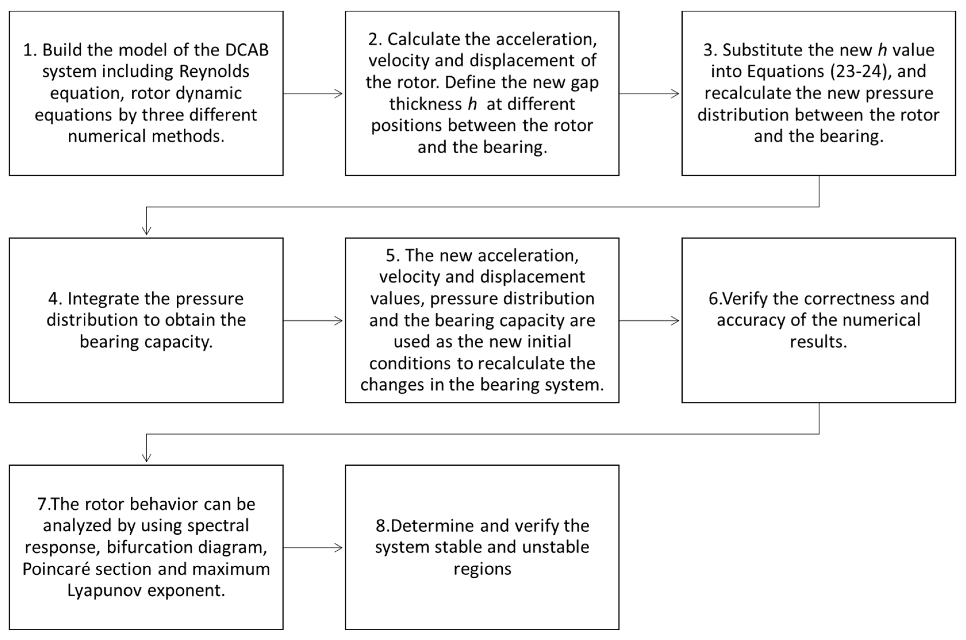
To calculate the dynamic behavior of the rotor center effectively, the acceleration of the rotor center is first calculated through the balance equation. Subsequently, the velocity and displacement are calculated. The aforementioned iterative calculation process begins from the initial static equilibrium state. The initial displacement of the rotor is determined by the static equilibrium position. Moreover, the gap thickness between the rotor and the bearing is determined. Assume that the initial velocity of the rotor is 0. The calculation process of the overall iteration (Figure 2) is described in the following text.
First step: After the time increment Δτ has passed, recalculate the acceleration, velocity, and displacement of the rotor. Moreover, define the new gap thickness value h at different positions between the rotor and the bearing.
Second step: Substitute the new h value into Equations (23) and (24). Then, recalculate the new pressure distribution state between the rotor and the bearing.
Third step: Integrate the pressure distribution calculated in step 2 to obtain the bearing capacity.
Fourth step: The new acceleration, velocity, and displacement values calculated in step 1; the pressure distribution calculated in step 2; and the bearing capacity obtained in step 3 are used as the new initial conditions for the next calculation. By using this new set of parameter conditions, return to the first step to recalculate the changes in the bearing system.
By using the aforementioned steps, the pressure variation and distribution inside the bearing system can be determined. The aforementioned steps can also be used to determine the relationship between the air film thickness and the position change at each time point, the change in the air film bearing capacity, and the dynamic behavior of the rotor.
In this study, to understand in detail the dynamic behavior of the DCAB system, the number of bearings (related to the rotor speed) and the rotor mass were used as bifurcation parameters and a bifurcation diagram was drawn for stability analysis. The dimensionless bearing number (Λ) is expressed as follows [15]:
Different numerical methods were used in this study to ensure the applicability and accuracy of the proposed hybrid method.
4. Results
4.1. Comparison of the Results Obtained with Different Numerical Methods
In this study, three numerical methods were used to solve the Reynolds equation of the DCAB system. The simulation results indicate that the hybrid scheme combining the DTM and FDM produced nearly identical results to the perturbation method and FDM. However, the rotor center displacements obtained with the perturbation method exhibited unstable numerical phenomena under specific operating conditions. The hybrid method exhibited a higher accuracy than the other two methods. Table 2 presents a comparison of the rotor center displacements (X2, Y2) obtained with the three adopted numerical methods for different mr and Λ values.
To determine and verify the stability of the numerical results, the influence of different time intervals on the results were studied. The rotor center displacements with periodic motions under specific conditions were also compared according to the values of the Poincaré sections (Table 3). As indicated by the numerical results, the hybrid method exhibited outstanding convergence and applicability for the DCAB system. The rotor trajectories for different operation parameters and time-step values () can be calculated to the fifth decimal place precisely when using the hybrid scheme. The rotor trajectories obtained with the hybrid scheme were superior to those obtained with the perturbation method and FDM (Table 2). The values of the Poincaré sections of the rotor center in the DCAB system for different time intervals are presented in Table 3. The results obtained with the hybrid method had an accuracy of calculation to the fifth right digit under different time increments. Thus, a small time step did not have to be used in this study to save calculation time and obtain high-precision calculation results for the DCAB system. Therefore, π/300 was used as the time interval in the subsequent dynamic analysis.
4.2. Dynamic Behavior of a DCAB System: Using the Rotor Mass as the Bifurcation Parameter
The rotor mass affects the strength of the air flotation effect between the rotor and the bearing, which is one of the key factors that influence the stability of the entire air-bearing system. Therefore, the influence of the rotor mass on the DCAB system was analyzed. In this section, the rotor mass (mr) is considered as the bifurcation parameter and the bearing number (Λ) of the system is considered to be 2.5.
4.2.1. Dynamic Trajectory and Phase Plane Analysis
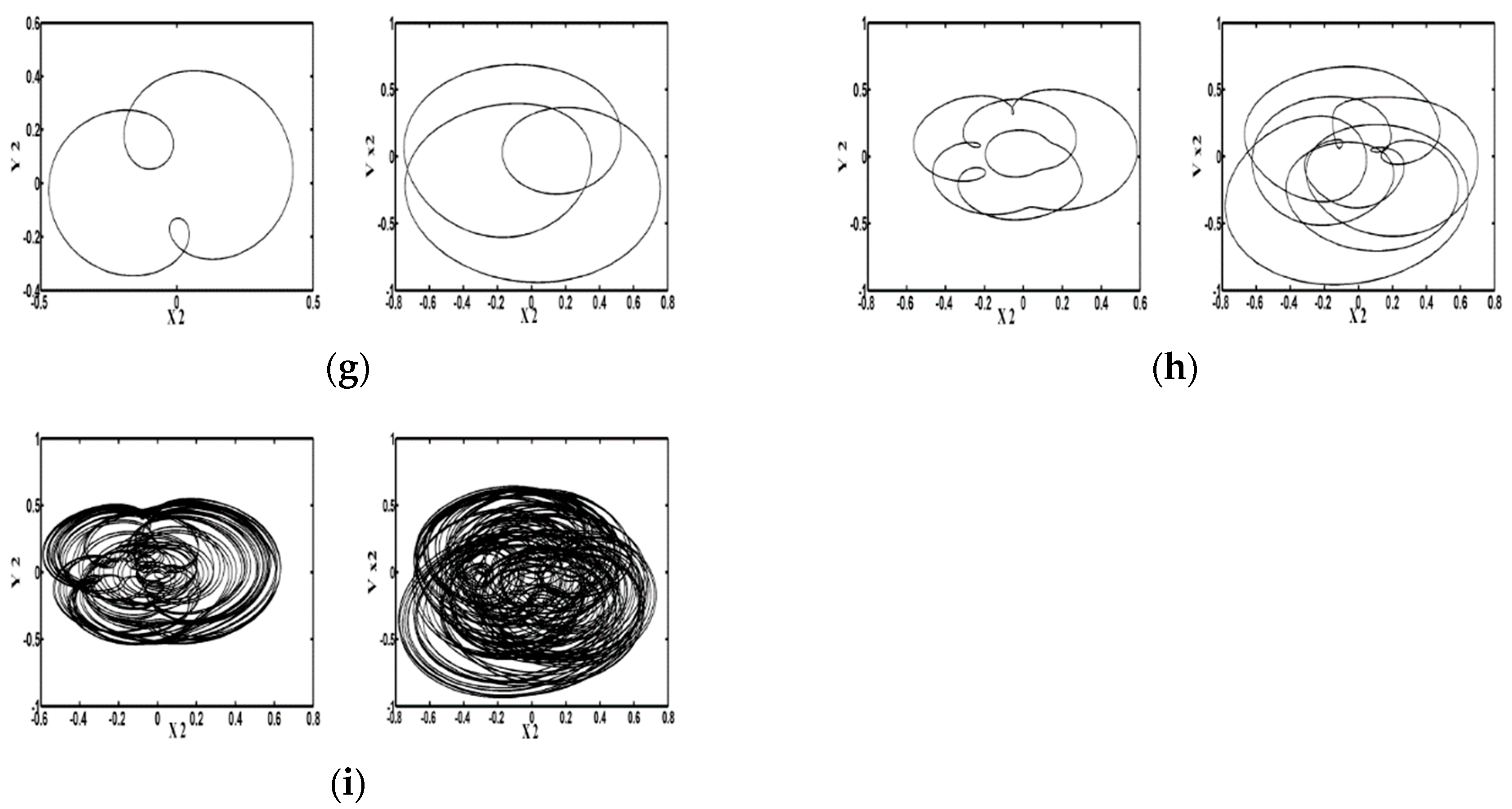
Figure 3 indicate that the rotor center (X2, Y2) has a regular trajectory for a low mass (mr = 11.2 kg). When the mass is increased to 20.92 kg, the regular motion changes to nonperiodic motion. When the rotor mass is maintained below 20.92 kg, the system is stable. The nonperiodic phenomenon becomes less obvious for rotor masses of 23.13, 24.31, 24.4, 24.52, 24.58, and 24.60 kg. When mr is 24.75 kg, the system suddenly becomes nonperiodic.
4.2.2. Spectral Analysis
Figure 4 illustrates the dynamic spectral responses of the rotor along the horizontal and vertical directions of the coordinate system. The results displayed in the aforementioned figures reveal that the rotor center exhibits T-periodic motion when the rotor mass is 11.2 kg. The spectral responses depicted in Figure 4b indicate that motion of the rotor center becomes quasi-periodic along the horizontal and vertical directions when mr is 20.92 kg. When the rotor mass is increased to 23.13, 24.4, or 24.58 kg, the system motion becomes T-periodic. At mr values of 24.31, 24.52, and 24.60 kg, the system exhibits subharmonic 3T-periodic motion. Moreover, when the rotor mass is increased to 24.75 kg, the system displays chaotic motion.
4.2.3. Bifurcation Analysis
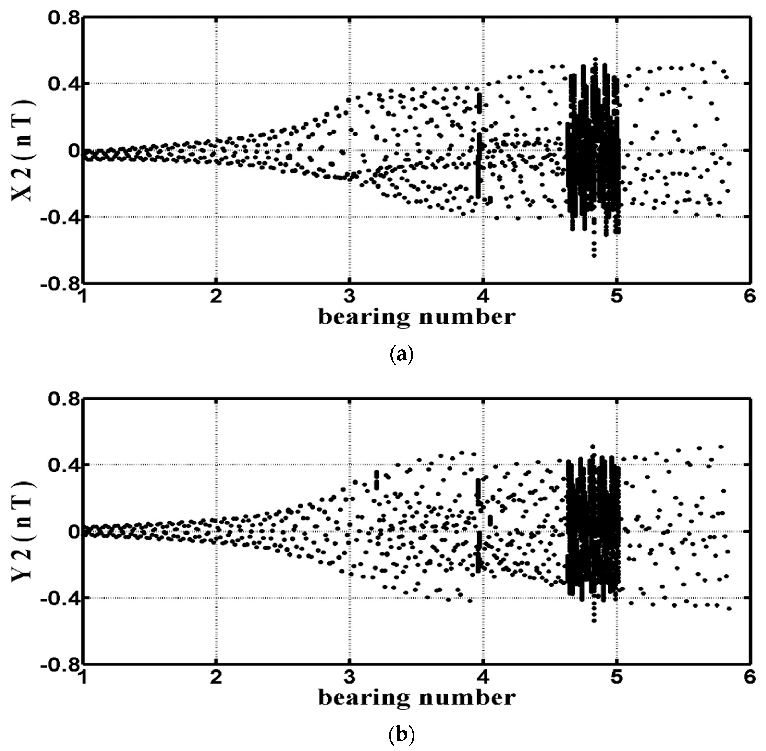
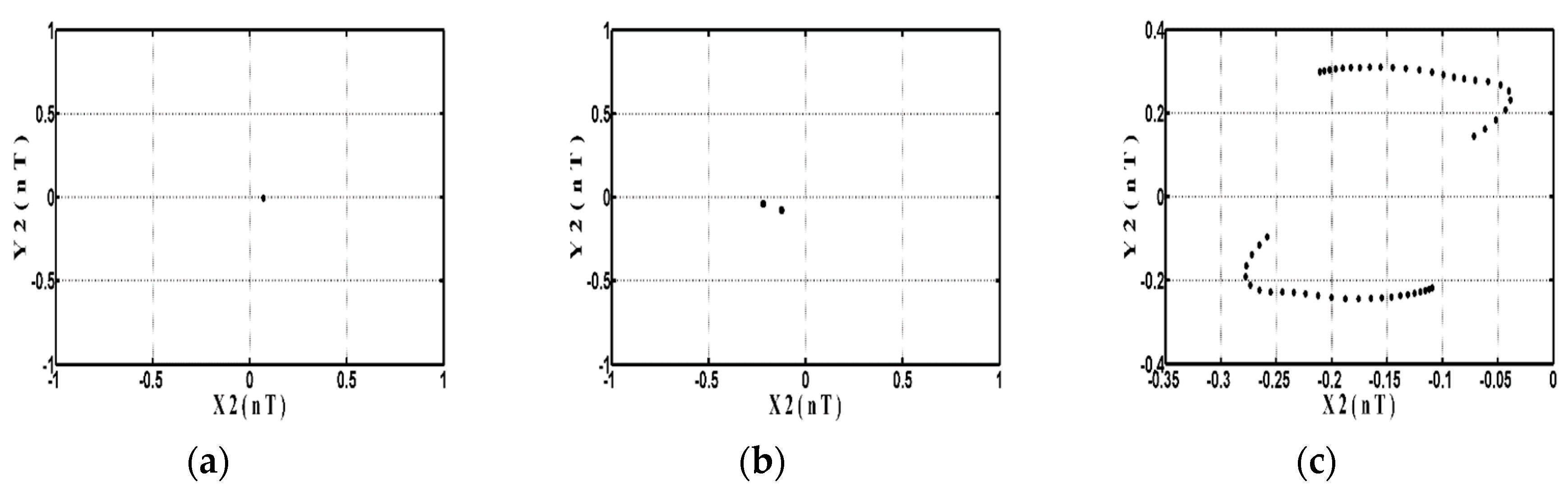
Figure 5 displays the influence of the rotor mass mr on the DCAB system. The rotor masses are set between 0.1 and 25.0 kg in the operation of the DCAB system. Figure 4a,c indicates that the rotor in the system exhibits T-periodic motion in the horizontal and vertical directions when mr is less than 20.92 kg. This phenomenon is confirmed by analyzing the Poincaré section [Figure 6a]. When the rotor mass is increased to 20.92 kg, the T-periodic motion is replaced by quasi-periodic motion, as displayed in Figure 5b,d. The aforementioned state of motion is illustrated by the closed curve formed by the discrete points in the Poincaré section [Figure 6b]. The aforementioned motion is observed for an mr range of 20.92–23.13 kg. When the rotor mass is decreased to 20.13 kg, the system again exhibits T-periodic motion [Figure 6c]. This periodic motion is observed in the mr range of 20.13–24.31 kg. When the rotor mass is 24.31 kg, the original T-periodic motion bifurcates into 3T-periodic motion, as depicted in Figure 6d, in which three discrete points can be observed on the map. The 3T-periodic motion is observed within an mr range of 24.31–24.4 kg. The 3T-periodic motion changes to T-periodic motion when the rotor mass is increased to 24.4 kg, as displayed in Figure 6e. T-periodic motion is observed within an mr range of 24.4–24.52 kg. The aforementioned description indicates that the T- and 3T-periodic motions occur alternately over an mr range of 24.52–24.75 kg, as depicted in Figure 6f,h.
When the rotor mass is increased to 24.75 kg, the original stable motion becomes nonperiodic, as illustrated in Figure 6i. Moreover, a number of irregular discrete points occur on the map. Nonperiodic motion occurs in the mr range of 24.75–25.0 kg. The types of rotor center behaviors for different rotor masses are presented in Table 4.
In this study, maximum Lyapunov exponents (MLEs) were used to identify and verify chaotic behavior. Figure 7a–h indicates that when mr is 11.2, 20.92, 23.13, 24.31, 24.4, 24.52, 24.58, or 24.60 kg, the MLEs approach or are smaller than 0. Thus, the system exhibits nonchaotic behavior for the aforementioned mr values. When mr is 24.75 kg, as depicted in Figure 7i, the values of the MLEs are greater than 0; thus, the DCAB system exhibits chaotic motion. The MLE distribution of the DCAB system is displayed in Figure 8. Figure 8 indicates that the blue curve, which indicates chaotic motion (the MLEs are greater than 0), occurs between 24.75 and 25.0 kg. The red curve, which represents the stable situation, matches the aforementioned results and indicates that the rotor exhibits complicated types of motions.
4.3. Dynamic Behavior of a DCAB System: Using the Bearing Number as the Bifurcation Parameter
The bearing number (Λ) directly influences not only the pressure distribution inside the bearing but also the rotational speed and stability of the DCAB system. In this section, the bearing number Λ is considered as the bifurcation parameter and the rotor mass mr is considered as 5.7 kg. The influence of Λ on the rotor dynamic behavior of the DCAB system is described in the following text.
4.3.1. Dynamic Trajectory and Phase Plane Analysis
Figure 9 indicates that the rotor displays regular behavior at low bearing numbers (Λ = 2.1 or 3.21). When Λ is increased to 3.96, the rotor center begins to exhibit irregular and asymmetric motion. When the bearing number is increased to 3.98, the dynamic motion changes to a more regular periodic motion. Moreover, when Λ = 4.63, nonperiodic motion reappears. When the bearing number is increased to 5.02, the system returns to regular behavior. The aforementioned results indicate that distinctive changes occur in the behavior of the system as the bearing number increases marginally from 3.96 to 3.98. The rotor motion is nonperiodic when Λ = 3.96 and periodic when Λ = 3.98. Thus, the DCAB system is very sensitive to the bearing number.
4.3.2. Spectral Analysis
Figure 10 illustrates the rotor center dynamic responses along the horizontal and vertical directions of the coordinate system for different bearing numbers. The rotor center displays T-periodic motion when the bearing number is 2.1 or 5.02. However, the spectral response indicates that when Λ = 3.96 or 4.63, the rotor center displays nonperiodic motion. Moreover, at bearing numbers of 3.21 and 3.98, the system motion becomes 2T-subperiodic.
4.3.3. Bifurcation Analysis
The bearing number Λ is a key parameter for exploring the behavior of the DCAB system (Figure 11). The bearing number is set between 1.0 and 6.0, and this range complies with real operating conditions. Initially, when Λ = 2.1, the rotor center performs T-periodic motion in the horizontal and vertical directions. This phenomenon is revealed and verified by the Poincaré section depicted in Figure 12a, which only has a single point. The system exhibits T-periodic motion when the bearing number is between 1.0 and 3.21. When the bearing number is increased to 3.21, the system motion bifurcates into 2T-periodic motion. Figure 12b indicates that the system generates two discrete points, and the 2T-periodic motion continues in the Λ range of 3.21–3.96. When the bearing number is between 3.96 and 3.98, the system exhibits chaotic motion (see Figure 12c), in which irregular discrete points are observed). When Λ is equal to 3.98, the chaotic motion changes to 2T-periodic motion (Figure 12d). The system exhibits 2T-periodic motion when 3.98 ≤ Λ < 4.63. It displays chaotic motion again when 4.63 ≤ Λ < 5.02, as displayed in Figure 11 and Figure 12e This unstable motion changes to stable T-periodic motion when Λ = 5.02. This stable motion is maintained until Λ = 6.0, as displayed in Figure 12f. The relationship between the rotor center behavior and Λ is complicated. All the system motions that occur when 1.0 ≤ Λ ≤ 6.0 are presented in Table 5.
The MLEs were also used to determine and verify if chaotic behavior is affected by changes in the bearing number. Figure 13a,b,d,f indicates that the MLEs are smaller than 0 when Λ = 2.1, 3.21, 3.98, and 5.02; thus, the system exhibits nonchaotic motion for the aforementioned Λ values. Figure 13c,e indicates that the MLEs are greater than 0 when Λ = 3.96 and 4.63; thus, the system exhibits chaotic motion for the aforementioned Λ values. The variations in the MLEs with the bearing number are illustrated in Figure 14. The results in Figure 14 indicate that the chaotic regions (where the MLEs are greater than 0) occur when 3.96 ≤ Λ < 3.98 and 4.63 ≤ Λ < 5.02.
4.4. Establishment of the Steady and Nonsteady Operation Regions of the DCAB System
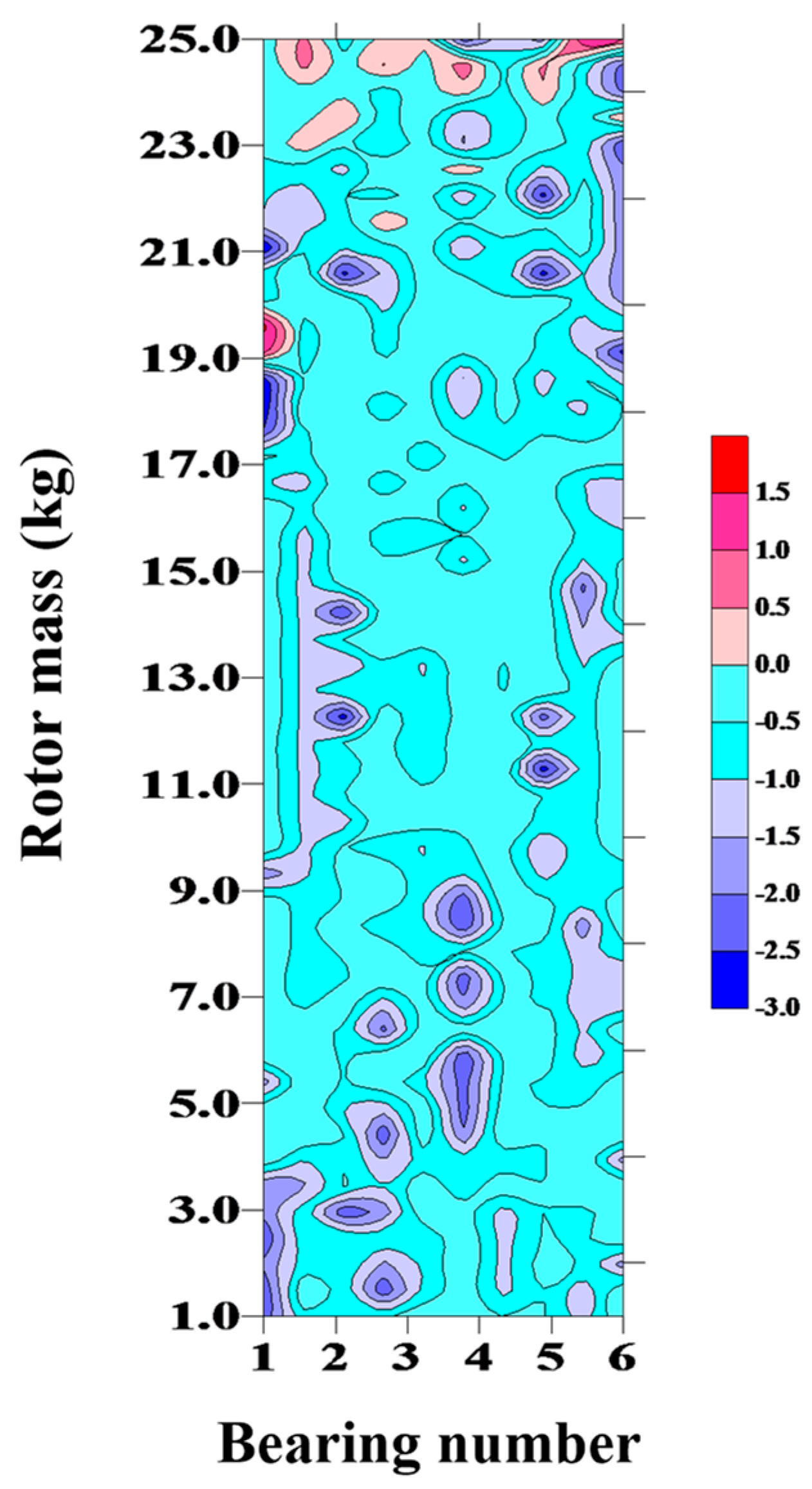
To determine if the behavior of the DCAB system is stable under various operating parameters, the rotor mass and bearing number were used as bifurcation parameters in the analysis conducted in this study. These two parameters influence the stability of the DCAB system. Moreover, their combined effect induces chaotic rotor behavior that cannot be predicted. Therefore, MLEs were used to confirm the stable and unstable operation regions for the DCAB system for different rotor masses and bearing numbers (Figure 15). In Figure 15, the light pink to deep red areas represent unstable regions, for which the MLEs are greater than 1.0. The light blue to deep blue areas represent stable regions, for which the MLEs are less than 0. The results in Figure 15 indicate that the unstable (chaotic) regions are concentrated in areas with a high rotor mass. The aforementioned results can be effectively used to identify the stable and unstable regions for avoiding chaotic motion in a DCAB system. These results also provide guidance for the design of bearing systems with high stability and performance.
5. Conclusions
The aims of this study were to analyze the various dynamic behaviors of the flexible rotor in the DCAB system under different operating parameters and to identify the stable and chaotic operation areas of the bearing system. The FDM, perturbation method, and hybrid method were used in the numerical analysis to determine the gas film pressure distribution and gas film thickness function of the Reynolds equation. The flexible rotor dynamic balance equation was then used to solve the trajectory displacement of the rotor center. Vibration signal analysis was performed by analyzing the spectral response generated by the displacement of the rotor center, Poincaré section diagram, bifurcation diagram, and MLEs. The numerical analysis results indicate that the hybrid method had a higher accuracy and precision than the FDM and perturbation method. Furthermore, a fairly accurate numerical solution could be obtained without using a small time step. The vibration analysis results indicate that the trajectory of the rotor center changes significantly with changes in the rotor mass and the bearing number. Changes in the aforementioned parameters produce various vibration behaviors in the horizontal and vertical directions, including periodic, subharmonic, quasi-periodic and chaotic motions. In particular, when the rotor mass is high, the bearing system exhibits unstable nonlinear chaotic behavior. Moreover, changes in the bearing number also affect the trajectory of the rotor. Chaotic behavior occurs when 3.96 ≤ Λ < 3.98 and 4.63 ≤ Λ < 5.02 for a rotor mass of 4.2 kg. When the bearing number does not fall within the aforementioned ranges, the rotor exhibits relatively stable motion. The major contribution of this study is its finding that the rotor mass and bearing number influence the stability of DCAB system. Furthermore, this study confirmed that the rotor exhibits chaotic behavior for specific ranges of the rotor mass and bearing number. The MLE is a key index for defining stable and unstable regions (nonchaotic and chaotic regions, respectively) for the DCAB system over various values of the rotor mass and bearing number. The research results can be used as an analysis reference and important basis for avoiding unstable nonlinear behaviors in DCAB system design and application.
Author Contributions
Conceptualization, methodology, validation, and writing—original draft preparation: C.-C.W. and writing—review and editing: C.-J.L. All authors have read and agreed to the published version of the manuscript.
Funding
This research was funded by the Ministry of Science and Technology of Taiwan (grant number: MOST-108-2221-E-167-028 and 108-2622-E-167-026-CC3).
Conflicts of Interest
The authors declare no conflict of interest.
References
- Reynolds, O. On the theory of lubrication and its application to Mr. Beauchamp tower’s experiments, including an axperimental determination of the viscosity of olive oil. Philos. Trans. R. Soc. Lond. Ser. A 1886, 177, 157–234. [Google Scholar]
- Whipple, R.T. The Inclined Groove Bearing; Atomic Energy Research Establishment: Harwell, UK, 1958. [Google Scholar]
- Whitley, S.; Williams, L.G. United Kingdom Atomic Energy Authority, I G Report 28(RD/CA); Industrial Group Headquarters: Risley, UK, 1959. [Google Scholar]
- Vohr, J.H.; Pan, C.H.T. On the Spiral-Grooved, Self-Acting, Gas Bearing; MTI Technical Report MTI63TR52, Prepared under Office of Naval Research Contract Nonr-3780(00), Task NR061-131; Mechanical Technology Inc.: Latham, NY, USA, 1964. [Google Scholar]
- Absi, J.; Bonneau, D. Caracteristiques statiques et dynamiques desPaliers a chevrons. In Proceedings of the 10 erne Congres Francois de Mecanique, Paris, France, 2–6 September 1991; Volume 1, pp. 253–256. [Google Scholar]
- Coleman, S.M. High capacity aerodynamic air bearing (HCAB) for laser scanning applications. In Optical Scanning: 31 Jul-1 Aug 2005; International Society for Optics and Photonics: San Diego, CA, USA, 2005; Volume 5873, pp. 56–64. [Google Scholar]
- Liu, Z.S.; Zhang, G.H.; Xu, H.J. Performance analysis of rotating externally pressurized air bearings. Proc. Inst. Mech. Eng. Part J J. Eng. Tribol. 2009, 223, 653–663. [Google Scholar] [CrossRef]
- Simek, J.; Lindovsky, P. Development of aerodynamic bearing support for application in air cycle machines. Appl. Comput. Mech. 2014, 8, 101–114. [Google Scholar]
- Bao, X.; Mao, J. Dynamic modeling method for air bearings in ultra-precision positioning stages. Adv. Mech. Eng. 2016, 8, 1–9. [Google Scholar] [CrossRef] [Green Version]
- Guo, P.; Gao, H. An active non-contact journal bearing with bi-directional driving capability utilizing coupled resonant mode. CIRP Ann. 2018, 67, 405–408. [Google Scholar] [CrossRef]
- Bently, D. Forced Subrotative Speed Dynamic Action of Rotating Machinery. In ASME Paper No. 74-PET-16, Proceedings of the Petroleum Mechanical Engineering Conference, Dallas, TX, USA, 15–18 September 1974; ASME: New York, NY, USA, 1974. [Google Scholar]
- Childs, D.W. Fractional-frequency rotor motion due to nonsymmetric clearance effects. ASME J. Eng. Gas Turbines Power 1982, 104, 533–541. [Google Scholar] [CrossRef]
- Wang, C.C. Non-periodic and chaotic response of three-multilobe air bearing system. Appl. Math. Model. 2017, 47, 859–871. [Google Scholar] [CrossRef]
- Wang, C.C.; Lee, T.E. Nonlinear dynamic analysis of bi-directional porous aero-thrust bearing systems. Adv. Mech. Eng. 2017, 9, 1–11. [Google Scholar] [CrossRef] [Green Version]
- Wang, C.C.; Lee, R.M.; Yau, H.T.; Lee, T.E. Nonlinear analysis and simulation of active hybrid aerodynamic and aerostatic bearing system. J. Low Freq. Noise Vib. Act. Control. 2019, 38, 1404–1421. [Google Scholar] [CrossRef] [Green Version]
- Zhang, S.; Zhang, S.; Wang, B.; Habetler, T.G. Machine learning and deep learning algorithms for bearing fault diagnostics—A comprehensive review. arXiv 2019, arXiv:1901.08247. [Google Scholar]
- Imani, M.; Ghoreishi, S.F. Bayesian optimization objective-based experimental design. In Proceedings of the 2020 American Control Conference (ACC), Denver, CO, USA, 1–3 July 2020; pp. 3405–3411. [Google Scholar]
- Ni, G.; Chen, J.; Wang, H. Degradation assessment of rolling bearing towards safety based on random matrix single ring machine learning. Saf. Sci. 2019, 118, 403–408. [Google Scholar] [CrossRef]
- Hashimoto, H.; Ochiai, M. Optimization of groove geometry for thrust air bearing to maximize bearing stiffness. ASME J. Tribol. 2008, 130, 031101. [Google Scholar] [CrossRef]
Figure 1.
Dual-directional coupled aerodynamic bearing (DCAB): (a) sectional view; (b) coordinate system.
Figure 1.
Dual-directional coupled aerodynamic bearing (DCAB): (a) sectional view; (b) coordinate system.
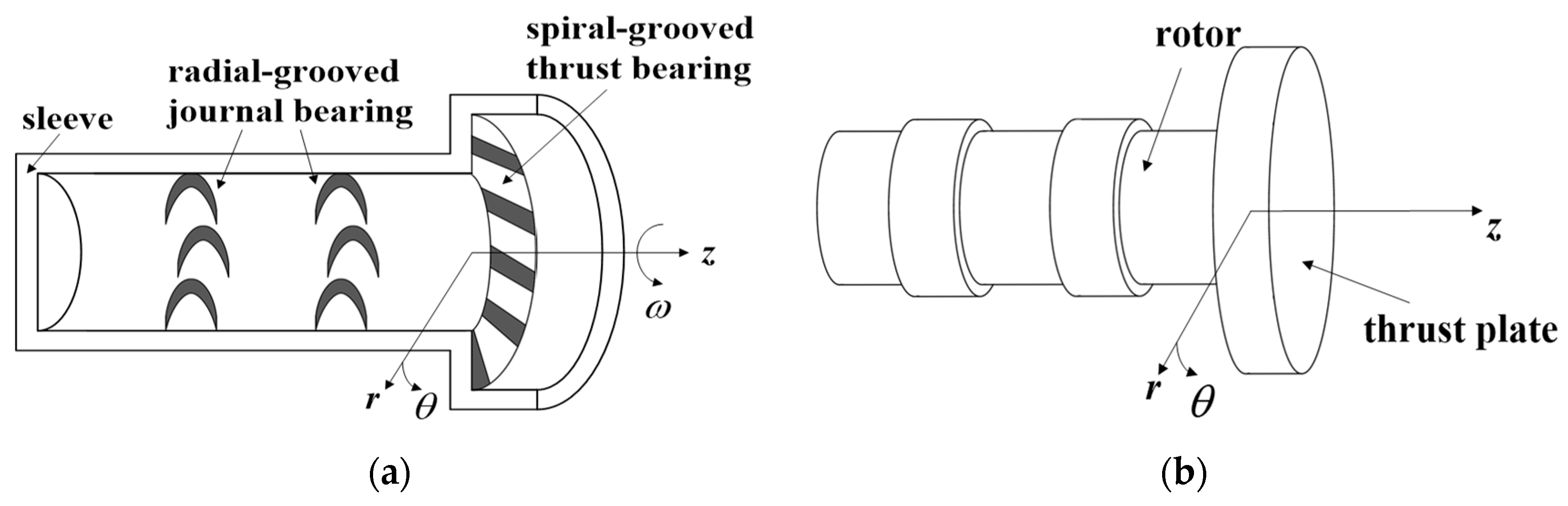
Figure 2.
Schematic of the calculation process.

Figure 3.
Dynamic trajectories (X2,Y2) and phase plots (X2,VX2) of the DCAB system for rotor masses of (a) 11.2, (b) 20.92, (c) 23.13, (d) 24.31, (e) 24.4, (f) 24.52, (g) 24.58, (h) 24.60, and (i) 24.75 kg and a bearing number of 2.5.
Figure 3.
Dynamic trajectories (X2,Y2) and phase plots (X2,VX2) of the DCAB system for rotor masses of (a) 11.2, (b) 20.92, (c) 23.13, (d) 24.31, (e) 24.4, (f) 24.52, (g) 24.58, (h) 24.60, and (i) 24.75 kg and a bearing number of 2.5.


Figure 4.
Spectral responses along the horizontal and vertical directions of the DCAB system for rotor masses of (a) 11.2, (b) 20.92, (c) 23.13, (d) 24.31, (e) 24.4, (f) 24.52, (g) 24.58, (h) 24.60, and (i) 24.75 kg and a bearing number of 2.5.
Figure 4.
Spectral responses along the horizontal and vertical directions of the DCAB system for rotor masses of (a) 11.2, (b) 20.92, (c) 23.13, (d) 24.31, (e) 24.4, (f) 24.52, (g) 24.58, (h) 24.60, and (i) 24.75 kg and a bearing number of 2.5.
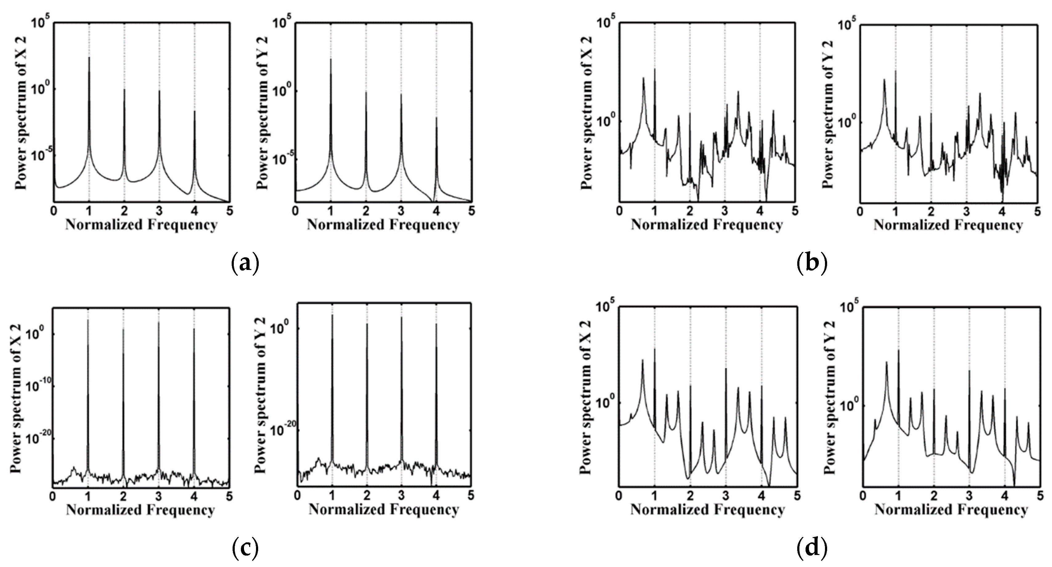
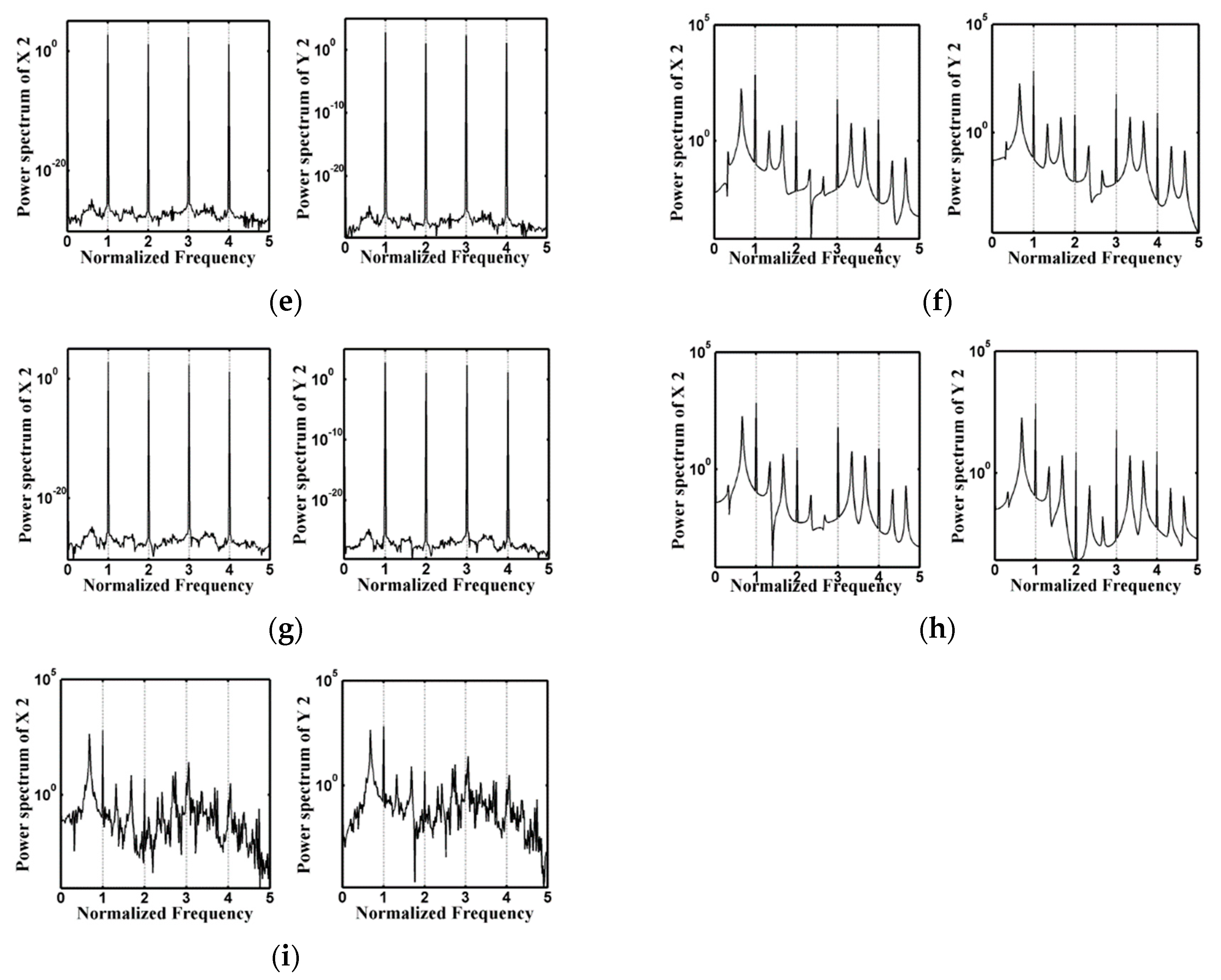
Figure 5.
Bifurcation diagrams of the rotor center in the DCAB system for different masses and a bearing number of 2.5: (a) X2(nT), (b) partial X2(nT), (c) Y2(nT), and (d) partial Y2(nT).
Figure 5.
Bifurcation diagrams of the rotor center in the DCAB system for different masses and a bearing number of 2.5: (a) X2(nT), (b) partial X2(nT), (c) Y2(nT), and (d) partial Y2(nT).
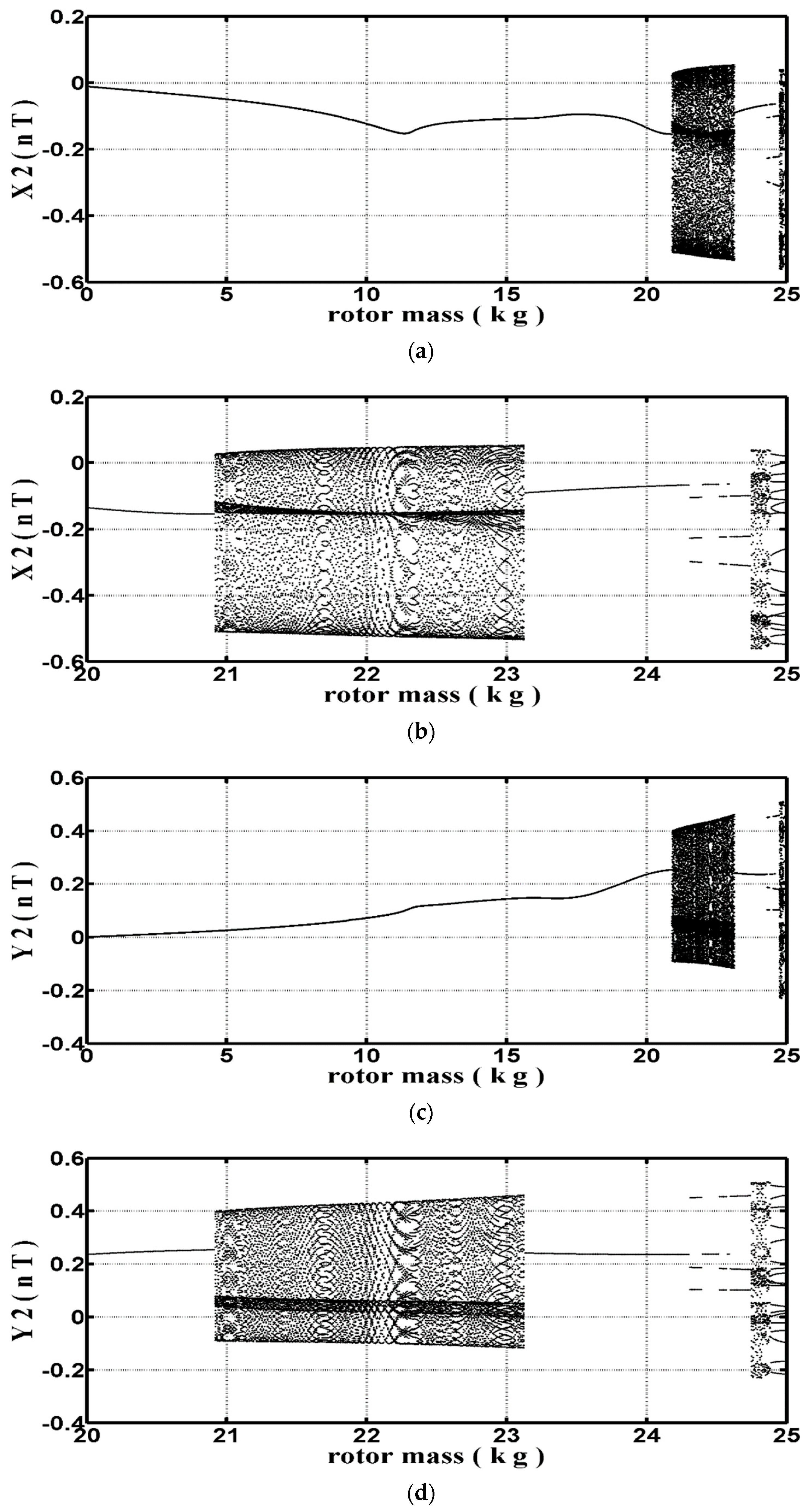
Figure 6.
Poincaré maps for different rotor masses: (a) mr = 11.2 kg, (b) mr = 20.92 kg, (c) mr = 23.13 kg, (d) mr = 24.31 kg, (e) mr = 24.4 kg, (f) mr = 24.52 kg, (g) mr = 24.58 kg, (h) mr = 24.60 kg, and (i) mr = 24.75 kg.
Figure 6.
Poincaré maps for different rotor masses: (a) mr = 11.2 kg, (b) mr = 20.92 kg, (c) mr = 23.13 kg, (d) mr = 24.31 kg, (e) mr = 24.4 kg, (f) mr = 24.52 kg, (g) mr = 24.58 kg, (h) mr = 24.60 kg, and (i) mr = 24.75 kg.
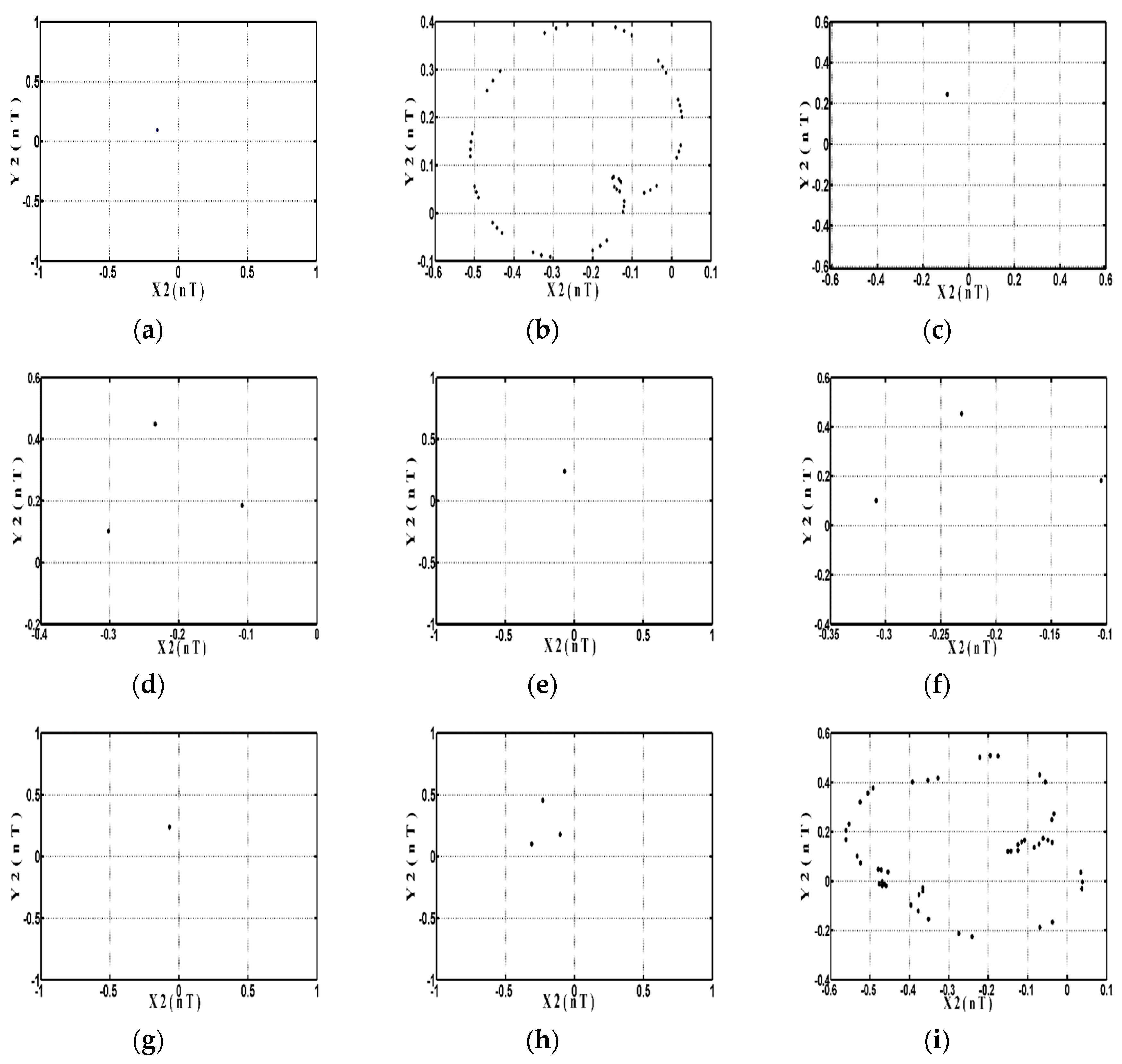
Figure 7.
Maximum Lyapunov exponents (MLEs) for different rotor masses: (a) mr = 11.2 kg, (b) mr = 20.92 kg, (c) mr = 23.13 kg, (d) mr = 24.31 kg, (e) mr = 24.4 kg, (f) mr = 24.52 kg, (g) mr = 24.58 kg, (h) mr = 24.60 kg, and (i) mr = 24.75 kg.
Figure 7.
Maximum Lyapunov exponents (MLEs) for different rotor masses: (a) mr = 11.2 kg, (b) mr = 20.92 kg, (c) mr = 23.13 kg, (d) mr = 24.31 kg, (e) mr = 24.4 kg, (f) mr = 24.52 kg, (g) mr = 24.58 kg, (h) mr = 24.60 kg, and (i) mr = 24.75 kg.

Figure 8.
Distribution of the MLEs for different rotor masses: (a) 0.1 ≤ mr ≤ 25.0 kg and (b) 24.0 ≤ mr ≤ 25.0 kg.
Figure 8.
Distribution of the MLEs for different rotor masses: (a) 0.1 ≤ mr ≤ 25.0 kg and (b) 24.0 ≤ mr ≤ 25.0 kg.


Figure 9.
Dynamic trajectories(X2,Y2) and phase plots(X2,VX2) of the DCAB system for bearing numbers of (a) 2.1, (b) 3.21, (c) 3.96, (d) 3.98, (e) 4.63, and (f) 5.02 with a rotor mass of 4.2 kg.
Figure 9.
Dynamic trajectories(X2,Y2) and phase plots(X2,VX2) of the DCAB system for bearing numbers of (a) 2.1, (b) 3.21, (c) 3.96, (d) 3.98, (e) 4.63, and (f) 5.02 with a rotor mass of 4.2 kg.


Figure 10.
Spectral responses along the horizontal and vertical directions of the DCAB system for bearing numbers of (a) 2.1, (b) 3.21, (c) 3.96, (d) 3.98, (e) 4.63, and (f) 5.02 with a rotor mass of 4.2 kg.
Figure 10.
Spectral responses along the horizontal and vertical directions of the DCAB system for bearing numbers of (a) 2.1, (b) 3.21, (c) 3.96, (d) 3.98, (e) 4.63, and (f) 5.02 with a rotor mass of 4.2 kg.
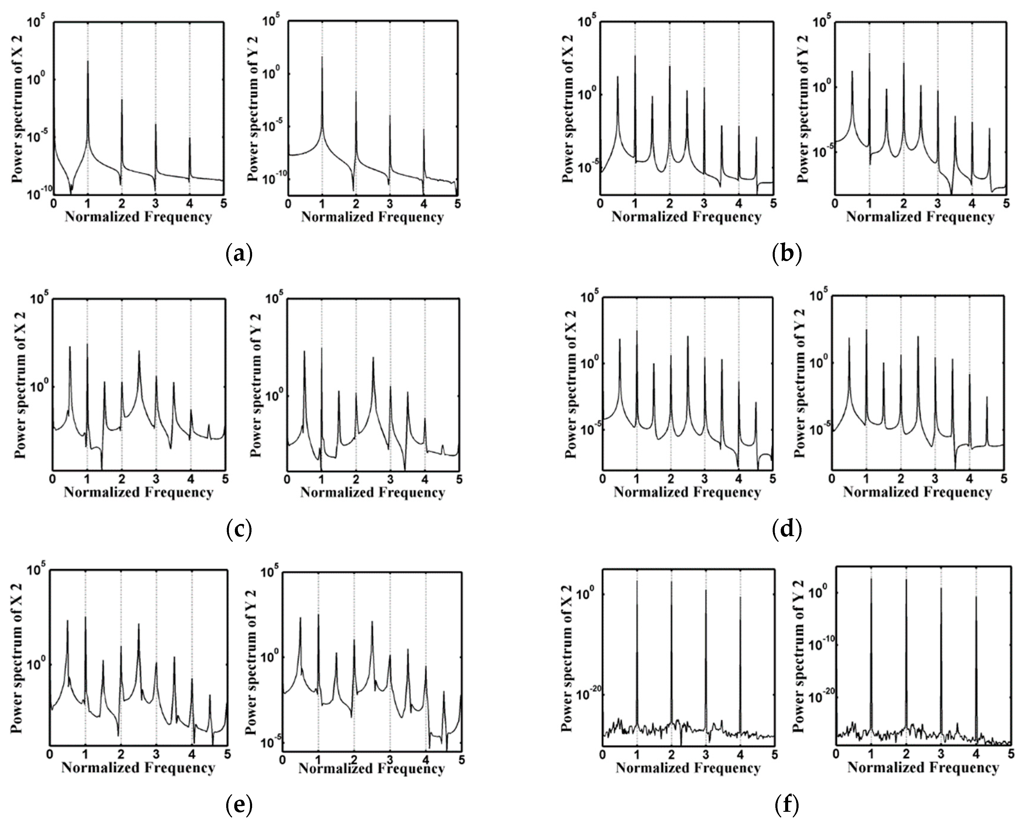
Figure 11.
Bifurcation diagrams for different bearing numbers when mr = 4.2 kg: (a) X2(nT) and (b) Y2(nT).
Figure 11.
Bifurcation diagrams for different bearing numbers when mr = 4.2 kg: (a) X2(nT) and (b) Y2(nT).

Figure 12.
Poincaré maps for different bearing numbers: (a) Λ = 2.1, (b) Λ = 3.21, (c) Λ = 3.96, (d) Λ = 3.98, (e) Λ = 4.63, and (f) Λ = 5.02.
Figure 12.
Poincaré maps for different bearing numbers: (a) Λ = 2.1, (b) Λ = 3.21, (c) Λ = 3.96, (d) Λ = 3.98, (e) Λ = 4.63, and (f) Λ = 5.02.


Figure 13.
Variation of the MLEs with the number of driving force cycles for different bearing numbers: (a) Λ = 2.1, (b) Λ = 3.21, (c) Λ = 3.96, (d) Λ = 3.98, (e) Λ = 4.63, and (f) Λ = 5.02.
Figure 13.
Variation of the MLEs with the number of driving force cycles for different bearing numbers: (a) Λ = 2.1, (b) Λ = 3.21, (c) Λ = 3.96, (d) Λ = 3.98, (e) Λ = 4.63, and (f) Λ = 5.02.

Figure 14.
Distribution of the MLEs for different bearing numbers.
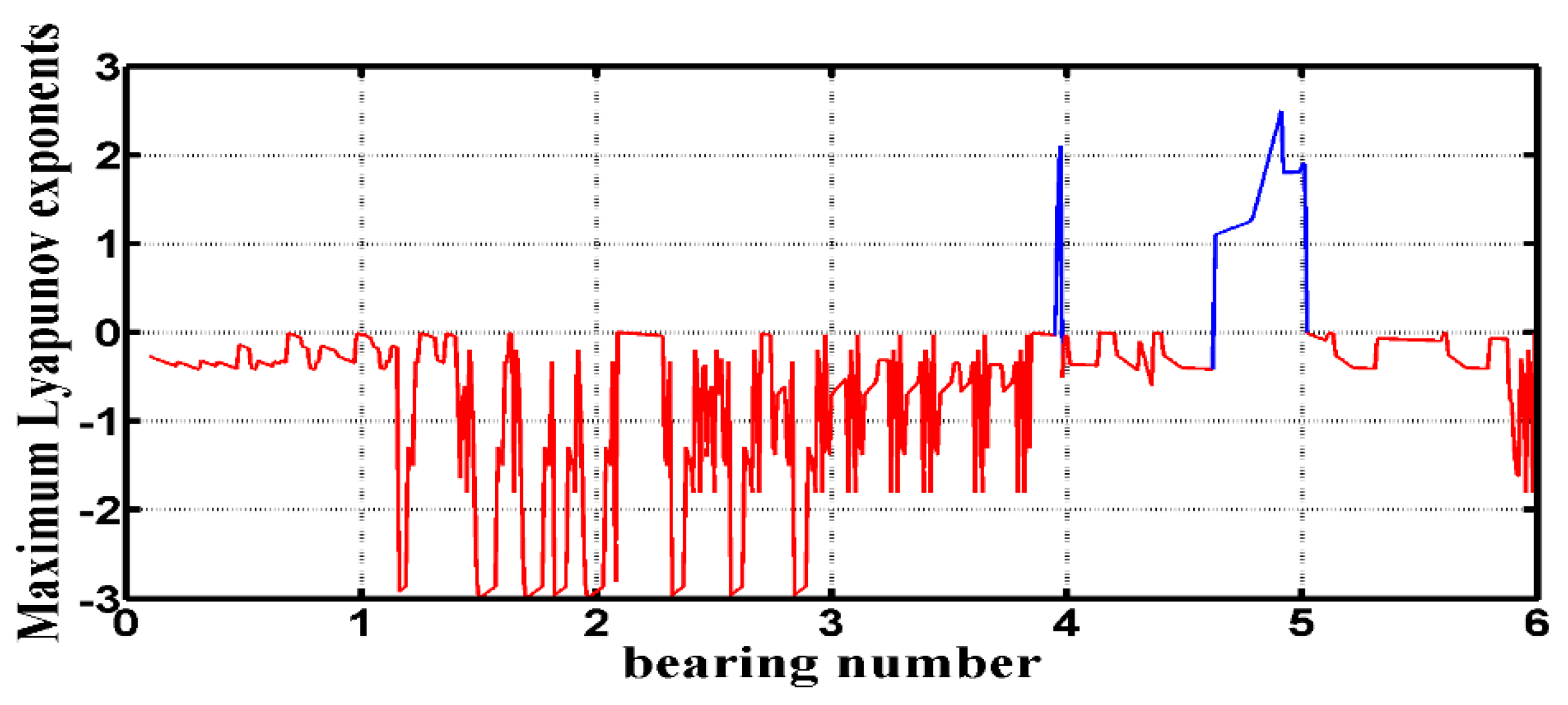
Figure 15.
Distribution of the MLEs for a DCAB system.

Table 1.
Nomenclature of the variables used in this study.
| Variable | Meaning |
|---|---|
| x, y, z, and | degrees of freedom for five directions |
| R | journal radius |
| L | bearing length |
| h | air film thickness |
| P | air film pressure |
| atmospheric pressure | |
| μ | viscosity coefficient |
| r,θ,z | coordinate system |
| t | time |
| physical quantity of perturbation | |
| rigidity of journal bearing and thrust bearing, respectively | |
| damping of journal bearing and thrust bearing, respectively | |
| mr | rotor mass |
| x2, y2 | displacements of rotor center |
| x3, y3 | displacements of journal center |
| rotational speed of rotor | |
| eccentricity of rotor | |
| stiffness coefficient of rotor | |
| equilibrium equation of forces acting to the journal center | |
| , , , ,,, | nondimensional group |
| time step | |
| Λ | dimensionless bearing number |
Table 2.
Comparison of the displacements of the rotor center obtained with the three adopted numerical methods for different mr and Λ values.
Table 2.
Comparison of the displacements of the rotor center obtained with the three adopted numerical methods for different mr and Λ values.
| Displacement | X2 | Y2 | |||
|---|---|---|---|---|---|
| Methods and Operating Conditions | |||||
| Perturbation method | mr = 11.2 kg Λ = 2.5 | −0.1823706379 | −0.1828876288 | 0.1788323797 | 0.1784390291 |
| Traditional finite-difference method | −0.1827916378 | −0.1826400484 | 0.1785890294 | 0.1788268449 | |
| Hybrid method | −0.1828351986 | −0.1828336582 | 0.1782085821 | 0.1782019995 | |
| Perturbation method | mr = 9.3 kg Λ = 2.5 | −0.1108152973 | −0.1100040131 | 0.0818502819 | 0.0810126263 |
| Traditional finite-difference method | −0.1106937267 | −0.1101360701 | 0.0811265030 | 0.0813032587 | |
| Hybrid method | −0.1105966888 | −0.1105993378 | 0.0812939956 | 0.0812912614 | |
| Perturbation method | mr = 5.7 kg Λ = 2.1 | 0.0743158143 | 0.0745814316 | −0.0022026672 | −0.0020779572 |
| Traditional finite-difference method | 0.0742887199 | 0.0740141869 | −0.0023085543 | −0.0024181594 | |
| Hybrid method | 0.07451222055 | 0.0745196645 | −0.0021489664 | −0.0021435547 | |
| Perturbation method | mr = 5.7 kg Λ = 3.0 | −0.2386678975 | −0.2384812317 | −0.0587582454 | −0.0582706309 |
| Traditional finite-difference method | −0.2389323073 | −0.2387243330 | −0.0585839042 | −0.0587359340 | |
| Hybrid method | −0.2385255159 | −0.2385242494 | −0.0584736366 | −0.0584706615 | |
Table 3.
Comparison of the values of the Poincaré sections of the rotor center in the DCAB system for different time intervals (τ; calculated using the hybrid method with mr = 5.6 kg and Λ = 2.5).
Table 3.
Comparison of the values of the Poincaré sections of the rotor center in the DCAB system for different time intervals (τ; calculated using the hybrid method with mr = 5.6 kg and Λ = 2.5).
| τ | X2(n T) | Y2(n T) |
|---|---|---|
| π/300 | −0.089320590874 | 0.052302554355 |
| π/600 | −0.089329265030 | 0.052301040131 |
Table 4.
Dynamic behaviors of the rotor center in the DCAB system for different rotor masses.
| Rotor Mass | [0.1, 20.92) | [20.92, 23.13) | [23.13, 24.31) | [24.31, 24.4) | [24.4, 24.52) |
| Dynamic Behavior | T | Quasi | T | 3T | T |
| Rotor Mass | [24.52, 24.58) | [24.58, 24.6) | [24.6, 24.75) | [24.75, 25.0] | |
| Dynamic Behavior | 3T | T | 3T | Chaotic |
Table 5.
Dynamic behavior of the rotor center in the DCAB system for different bearing numbers (1.0 ≤ Λ ≤ 6.0).
Table 5.
Dynamic behavior of the rotor center in the DCAB system for different bearing numbers (1.0 ≤ Λ ≤ 6.0).
| Λ | [1.0, 3.21) | [3.21, 3.96) | [3.96, 3.98) |
| Behavior | T | 2T | Chaos |
| Λ | [3.98, 4.63) | [4.63, 5.02) | [5.02, 6.0] |
| Behavior | 2T | Chaos | T |
© 2020 by the authors. Licensee MDPI, Basel, Switzerland. This article is an open access article distributed under the terms and conditions of the Creative Commons Attribution (CC BY) license (http://creativecommons.org/licenses/by/4.0/).
Share and Cite
MDPI and ACS Style
Wang, C.-C.; Lin, C.-J. Bifurcation and Nonlinear Behavior Analysis of Dual-Directional Coupled Aerodynamic Bearing Systems. Symmetry 2020, 12, 1521. https://doi.org/10.3390/sym12091521
AMA Style
Wang C-C, Lin C-J. Bifurcation and Nonlinear Behavior Analysis of Dual-Directional Coupled Aerodynamic Bearing Systems. Symmetry. 2020; 12(9):1521. https://doi.org/10.3390/sym12091521
Chicago/Turabian StyleWang, Cheng-Chi, and Chih-Jer Lin. 2020. "Bifurcation and Nonlinear Behavior Analysis of Dual-Directional Coupled Aerodynamic Bearing Systems" Symmetry 12, no. 9: 1521. https://doi.org/10.3390/sym12091521
Note that from the first issue of 2016, this journal uses article numbers instead of page numbers. See further details here.