The Generalized Bayes Method for High-Dimensional Data Recognition with Applications to Audio Signal Recognition

Abstract

High-dimensional data recognition problem based on the Gaussian Mixture model has useful applications in many area, such as audio signal recognition, image analysis, and biological evolution. The expectation-maximization algorithm is a popular approach to the derivation of the maximum likelihood estimators of the Gaussian mixture model (GMM). An alternative solution is to adopt a generalized Bayes estimator for parameter estimation. In this study, an estimator based on the generalized Bayes approach is established. A simulation study shows that the proposed approach has a performance competitive to that of the conventional method in high-dimensional Gaussian mixture model recognition. We use a musical data example to illustrate this recognition problem. Suppose that we have audio data of a piece of music and know that the music is from one of four compositions, but we do not know exactly which composition it comes from. The generalized Bayes method shows a higher average recognition rate than the conventional method. This result shows that the generalized Bayes method is a competitor to the conventional method in this real application.

1. Introduction

Recognizing high-dimensional data is an important problem in many applications, such as audio signal recognition, image analysis, and biological evolution. Especially, audio signal classification is an important high-dimensional data analysis problem. There are many tools that are established for audio signal classification. Convolutional neural network and tensor deep stacking network were used to sound classification [1]. A joint time-frequency approach was used in analyzing and extracting information from audio signals [2]. In this study, we focus on the high-dimensional data recognition problem when the data are assumed to follow Gaussian Mixture Models (GMMs). GMM is a very useful model that can be adopted in many real applications [3,4,5].

We use a musical data example to illustrate this recognition problem. Suppose that we have audio data of a piece of music and know that the music is from one of the four compositions, Beethoven’s Moonlight Sonata, Beethoven’s Minuet in G major, Beethoven’s Pastoral Symphony, or Beethoven’s Sonata Pathetique, but we do not know exactly which composition it comes from. To efficiently identify the composition that contains this piece of music, we can adopt signal recognition methods instead of a brute-force method. To adopt an audio signal recognition method, for each composition, we can use all the audio signal data or part of the audio signal data from this composition as training data to fit a high-dimensional GMM. After obtaining the four respective fitted GMMs for the four compositions, we can fit the audio data of this piece of music using these four GMMs, and find the GMM that best fits these data. The composition corresponding to this GMM is the composition to which this piece of music may belong.

We provide a general description of the method below. Suppose that we have K training samples, and each sample is assumed to follow a high-dimensional GMM with unknown parameters. These samples are used as training data to estimate the parameters of these K GMMs. Next, for a new sample that is known to be drawn from one of the K GMMs, we intend to find the valid GMM from which this sample is drawn. A conventional method applies the expectation-maximization (EM) algorithm to calculate the maximum likelihood estimator (MLE) of each GMM based on these training data [6,7]. After substituting these estimated parameter values into these GMMs, we can calculate the likelihood function value of each GMM based on this new sample. Next, we assign this new sample to the GMM with the highest likelihood function value. The rate of classifying the data to the valid model is called the recognition rate. For related studies on audio signal recognition or high dimensional data classification application, please refer to Reference [1,8,9,10].

In fact, the recognition rate mainly depends on the parameter estimation of the GMMs. Although the EM algorithm is a widely-used method to derive the MLEs of a GMM, it suffers from the local maxima problem and the initialization dependence problems. In addition to the MLE method, an alternative approach is to adopt Bayes estimators to estimate the parameters in the GMMs. The Bayesian approach has been widely-used in many applications, such as the response ranking problem in the survey data analysis and other areas [11].

By adopting a Bayes estimator, most studies focus on the Bayesian estimation, with respect to a proper prior [12,13,14]. A challenge of adopting a Bayes estimator, with respect to a proper prior is the selection of a suitable proper prior. In this study, we propose the use of a Bayes estimator, with respect to an improper prior (noninformative prior), which is called a generalized Bayes estimator [12], to estimate the parameters of GMMs. In addition, we compare these two methods under the frequentist framework. To the best of our knowledge, there are no reports in the literature regarding the use of the generalized Bayes estimator in GMMs for this recognition problem.

A procedure is given in Section 2 to obtain the generalized Bayes estimator. This procedure applies the Gibbs sampling method to calculate the generalized Bayes estimator and uses the k-means clustering method to find the initial values in the Gibbs sampling. We investigate the performance of this method by a simulation study and also by an actual real audio signal data application. The results show that the recognition rate obtained by the generalized Bayes estimator is higher than that obtained by the MLE method derived from the EM algorithm.

2. Methods

Suppose that we have K samples as training data, each with sample size n and drawn from a p-dimensional GMM. These training data are used to estimate the parameters of the K GMMs. The distribution of the $jth$ GMM has the form

$$\begin{array}{c}\hfill {\varphi }_{1j}N\left({\mathbf{u}}_{1j},{\Sigma }_{1j}\right)+{\varphi }_{2j}N\left({\mathbf{u}}_{2j},{\Sigma }_{2j}\right)+\cdots +{\varphi }_{mj}N\left({\mathbf{u}}_{mj},{\Sigma }_{mj}\right),\end{array}$$

(1)

where m is the component number, $N\left({\mathbf{u}}_{ij},{\Sigma }_{ij}\right)$ denotes a p-dimensional multivariate normal distribution with the means ${\mathbf{u}}_{ij}={(u_{ij1},\dots ,u_{ijp})}^{\prime }$ and covariance matrix ${\Sigma }_{ij}$, and ${\varphi }_{ij}^{\prime }s$ denote the proportions of the components in the GMM. The ${\varphi }_{ij}^{\prime }s$ satisfy ${\sum }_{i=1}^m{\varphi }_{ij}=1$ and ${\varphi }_{ij}\ge 0$. To simplify the notation, here, we consider a case in which each GMM has the same component number m. The methods used in this study can be directly applied to a case in which the K component numbers are different. In addition, to select a suitable component number for a GMM, we can apply model selection criteria, such as the Akaike information criterion (AIC) or other criteria, to find an appropriate component number.

Let ${\mathbf{y}}_{j1},\dots ,{\mathbf{y}}_{jn}$, where ${\mathbf{y}}_{jl}={(y_{jl1},\dots ,y_{jlp})}^{\prime },$ denote the training sample drawn from the $jth$ GMM, and we have K training samples $\{{\mathbf{y}}_{11},\dots {\mathbf{y}}_{1n}\},\dots \dots ,\{{\mathbf{y}}_{K1},\dots {\mathbf{y}}_{Kn}\}$ for the K GMMs. Assume that we have another new p-dimensional sample that is drawn from one of the K GMMs, and we are not aware of which model this sample is drawn from. The goal of this study is to find the true model from which this new sample is drawn.

Here, the parameters of interest are ${\theta }_j=\left\{\left({\mathbf{u}}_{ij},{\varphi }_{ij},{\Sigma }_{ij}\right)\mid i=1,\cdots ,m\right\},j=1,\dots ,K$. For a fixed j, to estimate the parameters ${\mathbf{u}}_{ij}$ and ${\Sigma }_{ij}$, we propose the use of generalized Bayes estimators, with respect to the Jeffreys prior

$$\begin{array}{c}{\pi }_1\left({\mathbf{u}}_{ij}\right)=I\left(-\infty <u_{ijh}<\infty \right),1\le i\le m,1\le h\le p\\ {\pi }_2\left({\Sigma }_{ij}\right)={\left|{\Sigma }_{ij}\right|}^{-(p+2)/2},1\le i\le m,\end{array}$$

(2)

where $I(·)$ denotes the indicator function, and $\left|A\right|$ denotes the determinant of the matrix A. The prior ${\pi }_1\left({\mathbf{u}}_{ij}\right)$ is symmetry for different dimensions because, for each dimension, the prior is $(-\infty ,\infty )$. For estimating the parameters ${\varphi }_{ij}$, we obtain an estimator of ${\varphi }_{ij}$ in the Gibbs sampling steps given below.

To calculate the generalized Bayes estimator, we utilize a natural invariant loss function. Let $X_1,\dots ,X_n$ be a random sample from a p-dimensional multivariate normal distribution $N_p(\mu ,\Sigma )$ and

$${\overline{X}}_n=\frac{1}{n}{\displaystyle \sum _{i=1}^n}{X}_{i}andS={\displaystyle \sum _{i=1}^n}(X_i-{\overline{X}}_n){(X_i-{\overline{X}}_n)}^{{}^{\prime }}.$$

The conditional posterior for $\mu$ and marginal posterior for $\Sigma$ under the Jeffreys prior are

$$\left(\mu \right|\Sigma ,X_1,\dots ,X_n)\sim N_p({\overline{X}}_n,\frac{1}{n}\Sigma )$$

and

$$\Sigma |X_1,\dots ,X_n\sim \mathrm{Inverse} \mathrm{Wishart}(S,n).$$

Under the entropy loss, defined by

$$L(\widehat{\mu },\widehat{\Sigma };\mu ,\Sigma )=(\widehat{\mu }-\mu ){\widehat{\Sigma }}^{-1}(\widehat{\mu }-\mu )+tr({\widehat{\Sigma }}^{-1}\Sigma )-log|{\widehat{\Sigma }}^{-1}\Sigma |-p,$$

the generalized Bayes estimators of $\mu$ and $\Sigma$ are

$${\widehat{\mu }}_B=E\left(\mu \right|X_1,\dots ,X_n)={\overline{X}}_n$$

and

$${\widehat{\Sigma }}_B=\frac{n+1}{n}E(\Sigma |X_1,\dots ,X_n)=\frac{(n+1)}{\left(n\right(n-p-1\left)\right)}S,$$

with respect to the Jeffreys prior (2) when p = 2 [15]. To provide a more simple form, we propose using $E\left(\mu \right|X_1,\dots ,X_n)$ and $E(\Sigma |X_1,\dots ,X_n)$ as estimators for estimating the mean and the covariance matrix of a multivariate normal distribution for each subgroup in the Gibbs sampler procedure introduced below. Although the result of Sun and Berger (2007) [15] is specific to the two dimensional case, the simulation results shown in Section 3 reveal that the proposed estimator also has good performance in higher dimensional cases.

To adopt the above result to GMMs, we apply the Gibbs sampler to calculate the generalized Bayes estimator, and derive the formulas in each step of the Gibbs sampler procedure. The Gibbs sampler is well-adapted to sampling the posterior distribution [16,17,18]. For implementing the Gibbs sampler, it is necessary to set the initial values of the parameters. The k-means algorithm is a popular method for cluster analysis in data mining [2,19]. We adopt this algorithm to select the initial values in the Gibbs sampler procedure. The data can be first approximately classified into several groups using the k-means approach.

To simplify the notation and without loss of generality, we consider the case of the first GMM model with $j=1$ in the procedure of Gibbs sampler below. Assume that we have training data ${\mathbf{y}}_{1l},l=1,\dots ,n$, for the first GMM. The Gibbs sampler approach is to associate with each observation ${\mathbf{y}}_{1l}$ a missing multinomial variable $z_l\sim {\mathcal{M}}_m(1;{\eta }_{l1},\cdots ,{\eta }_{lm})$ such that ${\mathbf{y}}_{1l}$ conditions on $z_l=h$ follows a normal distribution $N({\mathbf{u}}_{h1},{\Sigma }_{h1})$, where ${\mathcal{M}}_m(1;{\eta }_{l1},\cdots ,{\eta }_{lm})$ denotes a multinomial distribution with probabilities ${\eta }_{l1},\cdots ,{\eta }_{lm}.$ Using the random variables $z_l$, we can assign data ${\mathbf{y}}_{1l},l=1,\dots ,n$ to m groups and then estimate the mean and the covariance matrix for each subgroup. Thus, we have the following procedure for calculating the generalized Bayes estimator by the Gibbs sampler.

Procedure for calculating the generalized Bayes estimator of a GMM, with respect to prior (2).

The notation “count” below denotes the iteration number.

Step 1. Adopt the k-means approach to classify the observations ${\mathbf{y}}_{1l},l=1,\dots ,n$ to m groups. For an $i\in \{1,\dots ,m\}$, the sample mean ${\mathbf{u}}_{i1}^{\left(0\right)}$ and the sample covariance ${\Sigma }_{i1}^{\left(0\right)}$ of the data which are clustered to the ith group are used as the initial values for ${\mathbf{u}}_{i1}$ and ${\Sigma }_{i1}$, respectively. We can set an initial value for the ${\varphi }_{i1}$ to be the equal weight ${\varphi }_{i1}^{\left(0\right)}=1/m$ for $i=1,\dots ,m$.

Step 2. For each $l,l=1,\dots ,n$, obtain probabilities $({\eta }_{l1},\cdots ,{\eta }_{lm})$ in the multinomial distribution ${\mathcal{M}}_m(1;{\eta }_{l1},\cdots ,{\eta }_{lm})$ for the missing variable $z_l$ based on $({\mathbf{u}}_{i1}^{\left(0\right)},{\Sigma }_{i1}^{\left(0\right)},{\varphi }_{i1}^{\left(0\right)})$ values as follows. For $w=1,\dots ,m$, let

$$\begin{array}{ccc}\hfill {\eta }_{lw}^{\left(0\right)}& =& P\left(z_l=w\mid {\mathbf{u}}_{i1}^{\left(0\right)},{\Sigma }_{i1}^{\left(0\right)},{\varphi }_{i1}^{\left(0\right)},i=1,\dots ,m\right)\hfill \\ & =& \frac{{\varphi }_{w1}^{\left(0\right)}\frac{1}{{\left(2\pi \right)}^{\frac{p}{2}}\sqrt{|{\Sigma }_{w1}^{\left(0\right)}|}}exp\{-\frac{{({\mathbf{y}}_{1l}-{\mathbf{u}}_{w1}^{\left(0\right)})}^{\prime }{\left({\Sigma }_{w1}^{\left(0\right)}\right)}^{-1}({\mathbf{y}}_{1l}-{\mathbf{u}}_{w1}^{\left(0\right)})}{2}\}}{{\displaystyle \sum _{i=1}^m}{\varphi }_{i1}^{\left(0\right)}\frac{1}{{\left(2\pi \right)}^{\frac{p}{2}}\sqrt{|{\Sigma }_{i1}^{\left(0\right)}|}}exp\{-\frac{{({\mathbf{y}}_{1l}-{\mathbf{u}}_{i1}^{\left(0\right)})}^{\prime }{\left({\Sigma }_{i1}^{\left(0\right)}\right)}^{-1}({\mathbf{y}}_{1l}-{\mathbf{u}}_{i1}^{\left(0\right)})}{2}\}}.\hfill \end{array}$$

Next, we generate $z_l^{\left(0\right)}$ from the multinomial distribution ${\mathcal{M}}_m\left(1;{\eta }_{l1}^{\left(0\right)},{\eta }_{l2}^{\left(0\right)},\cdots ,{\eta }_{lm}^{\left(0\right)}\right)$ for $l=1,\dots ,n$.

Step 3. Let $n_i$ denote the number of $z_l^{(count-1)}$ equal to i for $i=1,\dots ,m$. If there exists an i such that $n_i=0$ for some i, go to Step 1 and redo the steps.

Let

$${\mathbf{u}}_{i1}^{\left(count\right)}=\sum _{\{l:z_l^{(count-1)}=i\}}\frac{{\mathbf{y}}_{1l}}{n_i^{(count-1)}},$$

$${\Sigma }_{i1}^{\left(count\right)}=\frac{1}{n-p-1}\sum _{\{l:z_l^{(count-1)}=i\}}({\mathbf{y}}_{1l}-{\mathbf{u}}_{i1}^{\left(count\right)}){({\mathbf{y}}_{1l}-{\mathbf{u}}_{i1}^{\left(count\right)})}^{{}^{\prime }}$$

and

$${\varphi }_{i1}^{\left(count\right)}=\frac{n_i^{(count-1)}}{n}.$$

Step 4. Let

$$\begin{array}{ccc}\hfill {\eta }_{lw}^{\left(count\right)}& =& p\left(z_l=w\mid {\mathbf{u}}_{i1}^{(count-1)},{\Sigma }_{i1}^{(count-1)},{\varphi }_{i1}^{(count-1)},i=1,\dots ,m\right)\hfill \\ & =& \frac{{\varphi }_{w1}^{(count-1)}exp\{-\frac{{({\mathbf{y}}_{l1}-{\mathbf{u}}_{w1}^{(count-1)})}^{\prime }{\left({\Sigma }_{w1}^{(count-1)}\right)}^{-1}({\mathbf{y}}_{l1}-{\mathbf{u}}_{w1}^{(count-1)})}{2}\}}{{\displaystyle \sum _{i=1}^m}{\varphi }_{i1}^{(count-1)}exp\{-\frac{{({\mathbf{y}}_{l1}-{\mathbf{u}}_{i1}^{(count-1)})}^{\prime }{\left({\Sigma }_{i1}^{(count-1)}\right)}^{-1}({\mathbf{y}}_{l1}-{\mathbf{u}}_{i1}^{(count-1)})}{2}\}}.\hfill \end{array}$$

Next, we generate $z_l^{\left(count\right)}$ from the multinomial distribution ${\mathcal{M}}_m\left(1;{\eta }_{l1}^{\left(count\right)},{\eta }_{l2}^{\left(count\right)},\cdots ,{\eta }_{lm}^{\left(count\right)}\right)$.

Step 5. Repeat Steps 3 and 4 for $count=c$. Let

$${\widehat{\mathbf{u}}}_{i1}=\frac{{\displaystyle \sum _{count=1}^c}{\mathbf{u}}_{i1}^{\left(count\right)}}{c},{\widehat{\Sigma }}_{i1}=\frac{{\displaystyle \sum _{count=1}^c}{\Sigma }_{i1}^{\left(count\right)}}{c},{\widehat{\varphi }}_{i1}=\frac{{\displaystyle \sum _{count=1}^c}{\varphi }_{i1}^{\left(count\right)}}{c}.$$

The ${\widehat{\mathbf{u}}}_{i1},{\widehat{\Sigma }}_{i1}$ and ${\widehat{\varphi }}_{i1}$ are used to estimate ${\mathbf{u}}_{i1},{\Sigma }_{i1}$ and ${\varphi }_{i1}$, respectively.

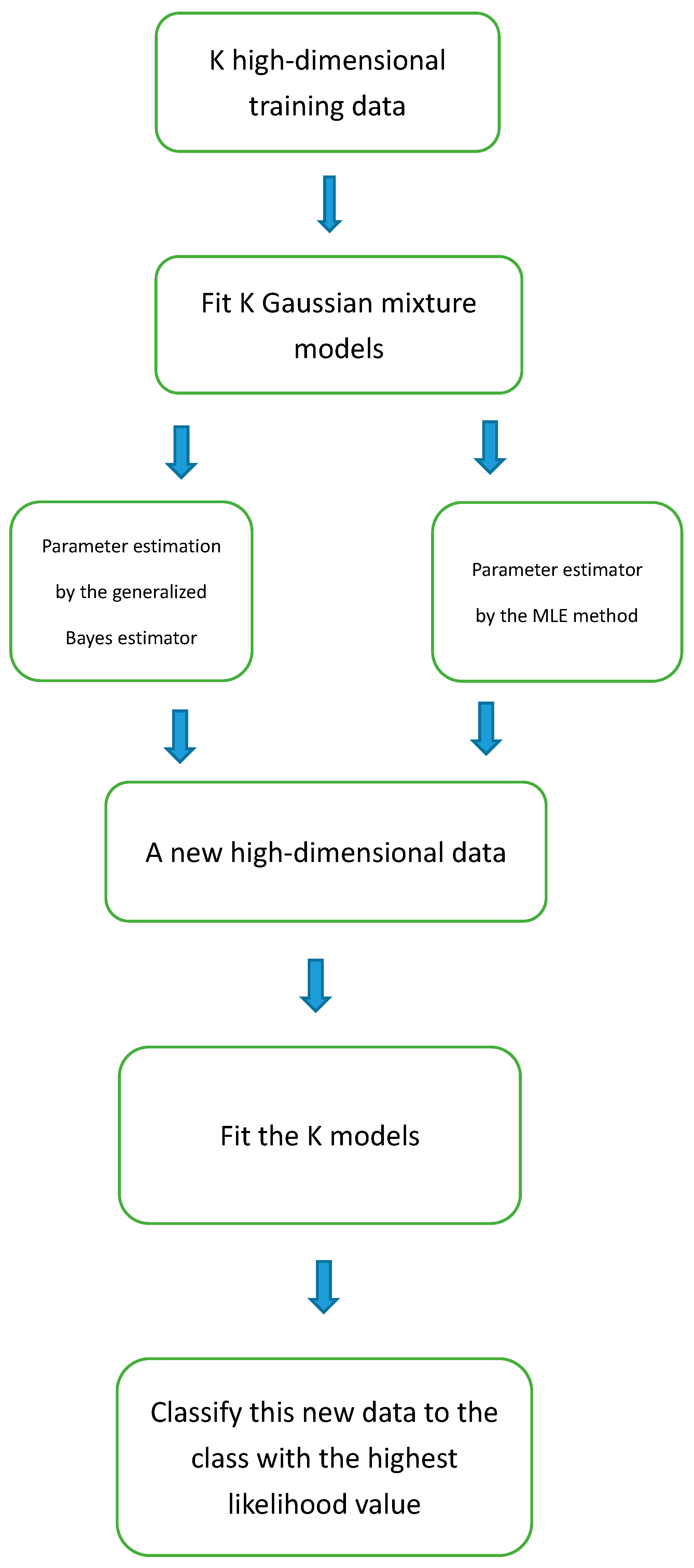
The flowchart of the classification is presented in Figure 1. In addition, according to Jasra, Holmes and Stephens (2005) [20], there are label switching problems in the Bayesian analysis of finite mixture models. The problems are mainly caused by the nonidentifiability of the components under symmetric priors [20,21]. To deal with the label switching problem, we may avoid this problem by checking the results of the iterations, and relabel them when a label switching occasion occurs.

3. Results and Discussion

3.1. Simulation

To compare the generalized Bayes method with the MLE method derived by the EM algorithm, we conduct a simulation study. The simulation is performed using MATLAB codes. The MLEs derived from the EM algorithm of a GMM are obtained using the MATLAB function gmdistribution.fit. The performances of the methods are evaluated in terms of the recognition rate, which is defined below. For a new sample ${\mathbf{y}}_{\mathbf{1}}^{*},\dots ,{\mathbf{y}}_{\mathbf{r}}^{*}(r>0),$ to classify it to one of the K models, we calculate the likelihood function values of this new sample for each model when the parameters in each GMM are estimated by the training data. Let $g_j({\widehat{\theta }}_j,t)$ denote the likelihood function of the $jth$ GMM, where ${\widehat{\theta }}_j$ are estimated based on the training data. There are a total of K likelihood function values associated with this sample. For a method, we classify this sample to the GMM with the largest likelihood function value, where the parameters are estimated by this method. That is, we classify this sample to the $vth$ GMM, where

$$\begin{array}{c}\hfill v=\arg {\max }_j{\mathbf{\Pi }}_{i=1}^{\mathbf{r}}{g}_j({\widehat{\theta }}_j,{\mathbf{y}}_{\mathbf{i}}^{*}).\end{array}$$

(3)

The recognition rate is the proportion that the data was classified to the valid model. In the simulation, we first generate a sample with size n for each GMM with given parameter values. Using these samples, we derive the maximum likelihood estimators and the generalized Bayes estimators for the parameters of each GMM. Next, we randomly select a GMM and generate a sample from this GMM. We repeat the above process 1000 times and each time the true parameter values are reset. Then, we calculate the proportion in the 1000 replications that the sample is assigned to the valid GMM.

Table 1. The recognition rates for the cases of $p=3,5$, and 6 when the component number of the Gaussian mixture models (GMMs) is known.

r	20	40	60	80
$n=100,K=3,m=2,p=3,w=1$
MLE	0.4884	0.5214	0.5152	0.5350
Generalized Bayes	0.5058	0.5621	0.5749	0.6427
$n=300,K=5,m=4,p=5,w=2$
MLE	0.4974	0.5925	0.6645	0.6463
Generalized Bayes	0.6103	0.7355	0.7781	0.8199
$n=500,K=3,m=2,p=3,w=1$
MLE	0.5703	0.6309	0.7000	0.7505
Generalized Bayes	0.5868	0.6870	0.8000	0.7921
$n=500,K=5,m=4,p=5,w=2$
MLE	0.5696	0.6548	0.6833	0.7280
Generalized Bayes	0.6526	0.7808	0.8115	0.8672
$n=1000,K=5,m=4,p=5,w=3$
MLE	0.7830	0.8749	0.9210	0.9620
Generalized Bayes	0.8240	0.9245	0.9680	0.9840
$n=1000,K=5,m=4,p=6,w=4$
MLE	0.8918	0.9632	0.9871	0.9913
Generalized Bayes	0.9333	0.9797	0.9940	0.9980
$n=2000,K=5,m=4,p=6,w=4$
MLE	0.9200	0.9766	0.9950	0.9944
Generalized Bayes	0.9390	0.9804	0.9970	0.9981
$n=2000,K=3,m=2,p=5,w=5$
MLE	0.9900	0.9970	1	1
Generalized Bayes	0.9920	0.9970	1	1

and

Table 2. The recognition rates for the cases of $p=15,20,25$, and 40 when the component number of the GMMs is known.

r	20	40	60	80
$n=1000,K=3,m=2,p=15,w=1$
MLE	0.5290	0.6161	0.7031	0.7389
Generalized Bayes	0.6160	0.7103	0.7241	0.8222
$n=1000,K=5,m=4,p=15,w=2$
MLE	0.5141	0.5834	0.7059	0.8658
Generalized Bayes	0.6396	0.6875	0.7353	0.9146
$n=1500,K=3,m=2,p=20,w=1$
MLE	0.5664	0.6030	0.6982	0.7420
Generalized Bayes	0.5929	0.6884	0.7658	0.8310
$n=1500,K=5,m=4,p=20,w=2$
MLE	0.5378	0.6067	0.6394	0.6735
Generalized Bayes	0.7198	0.7267	0.8115	0.8367
$n=2000,K=5,m=4,p=25,w=3$
MLE	0.7525	0.8043	0.8366	0.8537
Generalized Bayes	0.7921	0.8913	0.9543	0.9431
$n=2000,K=5,m=4,p=25,w=4$
MLE	0.8236	0.9554	0.9362	0.9912
Generalized Bayes	0.9510	0.9821	0.9912	1
$n=3000,K=5,m=4,p=40,w=4$
MLE	0.8273	0.9388	0.9386	0.9539
Generalized Bayes	0.9727	0.9728	0.9911	0.9923
$n=3000,K=3,m=2,p=40,w=5$
MLE	0.9935	1	1	1
Generalized Bayes	1	1	1	1

shows the recognition rates of the maximum likelihood method and the generalized Bayes method for different cases when the number m of clusters in each model is assumed to be known. The range of p for the simulation is from 3 to 40. The true parameters of GMMs used in Table 1 and Table 2 are selected by randomly generating ${\mathbf{u}}_{ij}$ from a p-dimensional uniform distribution, with each dimension following a uniform $U(0,w)$ distribution, and letting $\Sigma =V^{\prime }V+p{I}_p$, where V is a $p\times p$ matrix with each element generated from a uniform distribution $U(0,1)$, and $I_p$ is a p-dimensional identity matrix.

The simulation results in Table 1 and Table 2 show that the generalized Bayes approach improves the recognition rate compared with the MLE approach, especially when the training data sample size is not large. In Table 1 and Table 2, the sample size r of the test data is from 20 to 80. The recognition rates for both methods increase when r increases. We can see that the generalized Bayes approach is always better than the MLE method even when r is not large. In addition, there is a tendency that the improvement of the generalized Bayes approach increases when r increases. For example, in the first case in Table 1, the recognition rate increases from 0.4884 to 0.5350 for the MLE method, with increase 0.0466. The recognition rate increases from 0.5058 to 0.6427 for the generalized Bayes approach method, with increase 0.1369. Furthermore, we consider the dimension p from 3 to 40 in this simulation study. When p increases, the recognition rate for the generalized Bayes approach method has better improvement than the MLE method. For example, for the case of $n=2000,K=5,m=4,w=4$, and $r=20$, in Table 1, we can see that the recognition rates of the generalized Bayes approach and the MLE method are 0.9390 and 0.9200 for the case of $p=6$, respectively. In Table 2, we can see, for the case of $n=2000,K=5,m=4,w=4$, and $r=20$, the recognition rates of the generalized Bayes approach and the MLE method are 0.9510 and 0.8236 for the case of $p=25$, respectively. The improvements of the generalized Bayes approach are 0.0190 and 0.1274 for the cases of $p=6$ and $p=25$, respectively.

We also analyze the computational complexity of these two methods. The central processing unit (CPU) times for calculating the MLE and the generalized Bayes estimator with MATLAB codes are close and are not costly when the dimension and sample sizes are not large. For example, when $n=500,K=4,m=2,p=5$, and $r=80$, the calculating time for the MLE method of 40 iterations are about 0.014 s. In addition, in real applications, the component number m of GMMs is typically unknown.

Table 3. The recognition rates when the component number m is misspecified by s.

r	20	40	60	80
$n=500,K=3,m=2,p=3,w=1,s=4$
MLE n	0.6000	0.5860	0.6597	0.6732
Generalized Bayes	0.5000	0.7044	0.7571	0.7620
$n=1000,K=3,m=2,p=3,w=1,s=4$
MLE	0.5653	0.6833	0.7280	0.7540
Generalized Bayes	0.5859	0.7033	0.7050	0.8080
$n=1000,K=5,m=4,p=5,w=2,s=2$
MLE	0.6690	0.7750	0.8260	0.8580
Generalized Bayes	0.7120	0.8000	0.8670	0.8730
$n=2000,K=5,m=4,p=5,w=2,s=6$
MLE	0.6310	0.7350	0.7853	0.8430
Generalized Bayes	0.6880	0.8120	0.8863	0.9070

shows the recognition rates when m is misspecified, where s in Table 3 is the misspecified value of m. Although the component number is misspecified for these cases, the recognition rates are greater than 0.5 for all of the cases. In addition, the results reveal that the generalized Bayes method still has better performance than the MLE method for these misspecified component number cases.

In addition, to obtain the advantages of both methods, we may consider combining aspects of each of the methods, such as using the generalized Bayes estimator, as an initial value in the EM algorithm. However, it takes more time to perform this combined method.

To evaluate these two methods, we compare their performances in terms of the recognition rate because it is difficult to directly compare the mean estimator and the covariance matrix estimator due to the following. For example, when we consider a GMM with 3 components, in the simulation study, we first set the three true parameters for the means and covariance matrices. Next, we generate data from the GMM and obtain estimators using either the generalized Bayes method or the MLE method. If we directly compare the mean and covariance matrix estimators of these two methods, there is a problem regarding how to correspond the three sets of estimators to the three sets of true parameters. There are $3\times 2=6$ combinations by which the estimators correspond to the true parameters. In addition, we do not know which combination is suitable for use. This issue causes the difficulty in the comparison of the estimators for the mean and the covariance matrix. Therefore, it is not suitable to directly compare different estimators of the mean and the covariance matrix in a GMM.

3.2. A Real Data Example

In this section, we revisit the musical data example in the introduction section to illustrate the methods and present their performances on this real data application. In audio signal recognition, the signal data, are usually recorded in wav format and then converted to 13, 26, or 39 dimensional Mel-frequency cepstral coefficients (MFCCs), which are used as a perceptual weighting that more closely resembles how we perceive sounds [22,23].

We record 7 different pieces of music in wav format for each song of the 4 classical music songs and then transform the data to 13-dimensional MFCCs. A MATLAB function “wave2mfcc” can be used to transform the data to MFCCs [1]. The recorded time of each piece is approximately ten seconds. The sample size of MFCCs of a ten-second piece of music is approximately 600. Next, we use one of the 7 pieces of each song as training data to estimate the parameters of the GMM. Thus, we use a total of 4 pieces as training data to estimate the parameters of the 4 GMMs, and we use the other 24 pieces as testing data. The component number m in each GMM is set to 3.

To select a component number, we can use AIC to select a number. For example, a piece of Beethoven’s Moonlight Sonata has AIC values, 26,979, 26,298, 25,905, and 25,919 corresponding to component numbers 1, 2, 3, and 4, respectively. Therefore, we select the component number 3, which has the smallest AIC value among these models. However, it may not be the most suitable component number for other pieces of music. In this real data study, we use the GMMs with $m=3$. If the component number selected by the AIC criterion or other criteria is too large, to reduce the computing cost, we may select a model with the component number less than 5.

The process is repeated 7 times, and each time, we use different pieces of songs as the training data, with the remaining 24 pieces of songs used as the testing data. The recognition rates for the 7 times and their average recognition rates are presented in

Table 4. The recognition rates of different cases and the average recognition rates.

	1	2	3	4	5	6	7	Average Rate
MLE	0.708	0.792	0.708	0.792	0.75	0.708	0.667	0.732
Generalized Bayes	0.792	0.833	0.667	0.833	0.75	0.75	0.875	0.786

.

In this example, except in the third case, the generalized Bayes method has a higher recognition rate than the MLE method. The generalized Bayes method also has a higher average recognition rate than the MLE method. This result shows that the generalized Bayes method is a competitor to the MLE method in this real application. The computations are performed by MATLAB codes. The range of the CPU time for performing a method, which includes reading a wave file (10-second data), converting the wave data to 13-dimensional MFCC data and obtaining the parameter estimators of a GMM is from 0.036 s to 0.056 s, with an average CPU time 0.046 s. Both methods require similar amounts of CPU time.

4. Conclusions

In this study, a generalized Bayes estimator of a GMM was proposed and was shown to improve the high-dimensional Gaussian mixture data recognition rate. In addition, a procedure for calculating the generalized Bayes estimator was provided. In this study, due to the complexity of GMMs, we only provided the simulation results instead of a theoretical inference to compare these two methods. Nevertheless, the generalized Bayes approach was shown to be an admissible estimator or a minimax estimator in other distributions [12,14]. Although it remains unknown whether the generalized Bayes estimator is an admissible estimator in GMM, the simulation and the real data case studies both show that the generalized Bayes approach is a method that is competitive with the MLE method.

References

- Khamparia, A.; Gupta, D.; Nguyen, N.G.; Khanna, A.; Pandey, B.; Tiwari, P. Sound classification using convolutional neural network and tensor deep stacking network. IEEE Access 2019, 7, 7717–7727. [Google Scholar] [CrossRef]
- Umapathy, K.; Ghoraani, B.; Krishnan, S. Audio signal processing using time-frequency approaches: Coding, classification, fingerprinting, and watermarking. EURASIP J. Adv. Signal Process. 2010, 2010, 1–28. [Google Scholar] [CrossRef] [Green Version]
- Chen, C.; Wang, H. Tolerance interval for the mixture normal distribution. J. Qual. Technol. 2019, 52, 145–154. [Google Scholar] [CrossRef]
- Roy, A.; Parui, S.K.; Roy, U. SWGMM: A semi-wrapped Gaussian mixture model for clustering of circular–linear data. Pattern Anal. Appl. 2016, 19, 631–645. [Google Scholar] [CrossRef]
- Müller, M. Information Retrieval for Music and Motion; Springer: Heidelberg, Germany, 2007; Volume 2. [Google Scholar]
- Dempster, A.P.; Laird, N.M.; Rubin, D.B. Maximum likelihood from incomplete data via the EM algorithm. J. R. Stat. Soc. Ser. B 1977, 39, 1–38. [Google Scholar]
- Jang, R. Speech and Audio Processing Toolbox. 2005. Available online: http://mirlab.org/jang/matlab/toolbox/sap (accessed on 1 December 2020).
- Chen, Z.S.; Jang, J.S.R. On the Use of Anti-word Models for Audio Music Annotation and Retrieval. IEEE Trans. Audio Speech Lang. Process. 2009, 17, 1547–1556. [Google Scholar] [CrossRef]
- Domeniconi, C.; Gunopulos, D.; Ma, S.; Yan, B.; Al-Razgan, M.; Papadopoulos, D. Locally adaptive metrics for clustering high dimensional data. Data Min. Knowl. Discov. 2007, 14, 63–97. [Google Scholar] [CrossRef]
- Punzo, A. A new look at the inverse Gaussian distribution with applications to insurance and economic data. J. Appl. Stat. 2019, 46, 1260–1287. [Google Scholar] [CrossRef]
- Wang, H.; Huang, W.H. Bayesian Ranking Responses in Multiple Response Questions. J. R. Stat. Soc. Ser. A (Stat. Soc.) 2014, 177, 191–208. [Google Scholar] [CrossRef]
- Berger, J. Statistical Decision Theory and Bayesian Analysis; Springer: New York, NY, USA, 1985. [Google Scholar]
- Ghosh, P.; Tang, X.; Ghosh, M.; Chakrabarti, A. Asymptotic Properties of Bayes Risk of a General Class of Shrinkage Priors in Multiple Hypothesis Testing Under Sparsity. Bayesian Anal. 2016, 11, 753–796. [Google Scholar] [CrossRef]
- Reynolds, D.; Rose, R.C. Robust Text-Independent Speaker Identification Using Gaussian Mixture Speaker Models. IEEE Trans. Speech Audio Process. 1995, 3, 72–83. [Google Scholar] [CrossRef] [Green Version]
- Smith, A.F.M.; Roberts, G.O. Bayesian computation via the Gibbs sampler and related Markov chain Monte Carlo methods. J. Royal Stat. Soc. Ser. B 1993, 55, 3–23. [Google Scholar] [CrossRef]
- Diebolt, J.; Robert, C.P. Estimation of finite mixture distributions through Bayesian sampling. J. R. Stat. Soc. Ser. B 1994, 56, 363–375. [Google Scholar] [CrossRef]
- Gelfand, A.E. Smith, A.F. Sampling based approaches to calculating marginal densities. J. Am. Stat. Assoc. 1990, 85, 398–409. [Google Scholar] [CrossRef]
- Robert, C. The Bayesian Choice. Springer Texts in Statistics; Springer: New York, NY, USA, 2001. [Google Scholar]
- Kanungo, T.; Mount, D.M.; Netanyahu, N.S.; Piatko, C.D.; Silverman, R.; Angela, Y.; Wu, A.Y. An Efficient k-Means Clustering Algorithm: Analysis and Implementation. IEEE Trans. Pattern Anal. Mach. Intell. 2002, 24, 881–892. [Google Scholar] [CrossRef]
- Jasra, A.; Holmes, C.; Stephens, D. Markov chain Monte Carlo methods and the label switching problem in Bayesian mixture modeling. Stat. Sci. 2005, 20, 50–67. [Google Scholar] [CrossRef]
- Aitkin, M. Likelihood and Bayesian analysis of mixtures. Stat. Model. 2001, 1, 287–304. [Google Scholar] [CrossRef]
- McLachlan, G.; Peel, D. Finite Mixture Models; Wiley: Hoboken, NJ, USA, 2000. [Google Scholar]
- Morgan, N.; Bourlard, H.; Hermansky, H. Automatic Speech Recognition: An Auditory Perspective. In Speech Processing in the Auditory System; Springer: New York, NY, USA, 2004; pp. 309–338. [Google Scholar]
Figure 1.
The flowchart of the classification.