Linear Energy Density and the Flux of an Electric Field in Proca Tubes

Abstract

In this work, we study cylindrically symmetric solutions within SU(3) non-Abelian Proca theory coupled to a Higgs scalar field. The solutions describe tubes containing either the flux of a color electric field or the energy flux and momentum. It is shown that the existence of such tubes depends crucially on the presence of the Higgs field (there are no such solutions without this field). We examine the dependence of the integral characteristics (linear energy and momentum densities) on the values of the electromagnetic potentials at the center of the tube, as well as on the values of the coupling constant of the Higgs scalar field. The solutions obtained are topologically trivial and demonstrate the dual Meissner effect: the electric field is pushed out by the Higgs scalar field.

1. Introduction

In quantum chromodynamics (QCD), it is assumed that the color non-Abelian fields between quark and anti-quark are confined in a tube due to a strong nonlinear interaction between different components of such fields. The properties of this tube are such that outside the tube, all fields, and hence the energy density, decrease exponentially with distance. Inside such a tube, there is a longitudinal electric field connecting quarks and attracting them to each other; this is the explanation of quark confinement. In classical SU(3) non-Abelian Yang–Mills theory uncoupled to other fields, such solutions are apparently absent. In turn, the lattice calculations in QCD indicate that such configurations of non-Abelian fields do exist; when other fields are involved, such solutions are already present. For example, when an electromagnetic field interacts with the Higgs scalar field, there exist tubes possessing a flux of a magnetic field—the well-known solutions found by Nielsen and Olesen [1]. Non-Abelian flux tube solutions with the flux of a magnetic field whose force lines are twisted along the tube axis have been obtained in [2].

Another interesting fact is that such tubes can exist in Proca theories. For example, in [3], it was shown that there exist gravitating and nongravitating Q-tubes supported by a complex vector field with nonlinear terms which can in some sense imitate the self-interaction in non-Abelian Yang–Mills theory. In [4,5], the existence of tubes within SU(3) Proca theory coupled to a Higgs scalar field has been demonstrated. In those papers, two types of tube solutions have been found. In the tubes of the first type, there is a flux of a longitudinal color electric field along the tube created by color charges (quarks) located at $\pm \infty$. In the tubes of the second type, there is a momentum directed along the tube. The presence of such a momentum is apparently equivalent to the presence of the energy flux transferred along the tube.

In the present paper, we continue our investigations in this direction. In doing so, we calculate integral characteristics of the solutions such as the total flux of the non-Abelian longitudinal Proca electric field, the linear energy density and the total momentum passing across the cross section of the tube, depending on the system parameters.

2. Non-Abelian-SU(3)-Proca-Higgs Theory

The Lagrangian that describes a system supported by a non-Abelian SU(3) Proca field $A_{\mu }^a$ interacting with nonlinear scalar field $\varphi$ can be taken in the form (hereafter, we work in units such that $c=\hslash =1$)

$$\mathcal{L}=-\frac{1}{4}{F}_{\mu \nu }^a{F}^{a\mu \nu }-\frac{{\left({\mu }^2\right)}_{\phantom{ab,}\nu }^{ab,\mu }}{2}{A}_{\mu }^a{A}^{b\nu }+\frac{1}{2}{\partial }_{\mu }\varphi {\partial }^{\mu }\varphi +\frac{\lambda }{2}{\varphi }^2{A}_{\mu }^a{A}^{a\mu }-\frac{\Lambda }{4}{\left({\varphi }^2-M^2\right)}^2.$$

(1)

where $F_{\mu \nu }^a={\partial }_{\mu }{A}_{\nu }^a-{\partial }_{\nu }{A}_{\mu }^a+g{f}_{abc}{A}_{\mu }^b{A}_{\nu }^c$ is the field strength tensor for the Proca field, $f_{abc}$ are the SU(3) structure constants, g is the coupling constant, $a,b,c=1,2,\dots ,8$ are color indices, $\mu$ and $\nu =0,1,2,3$ are spacetime indices. The Lagrangian (1) also contains the arbitrary constants $M,\lambda ,\Lambda$ and the Proca field mass matrix ${\left({\mu }^2\right)}_{\phantom{ab,}\nu }^{ab,\mu }$.

Using (1), the corresponding field equations can be written in the form

$$\begin{array}{ccc}\hfill D_{\nu }{F}^{a\mu \nu }-\lambda {\varphi }^2{A}^{a\mu }& =& -{\left({\mu }^2\right)}_{\phantom{ab,}\nu }^{ab,\mu }{A}^{b\nu },\hfill \end{array}$$

(2)

$$\begin{array}{ccc}\hfill \square \varphi & =& \lambda A_{\mu }^a{A}^{a\mu }\varphi +\Lambda \varphi \left(M^2-{\varphi }^2\right),\hfill \end{array}$$

(3)

and the energy density is

$$\begin{array}{cc}\hfill \epsilon =& \frac{1}{2}{\left(E_i^a\right)}^2+\frac{1}{2}{\left(H_i^a\right)}^2-\left[{\left({\mu }^2\right)}_{\phantom{ab,}0}^{ab,\alpha }{A}_{\alpha }^a{A}_0^b-\frac{1}{2}{\left({\mu }^2\right)}_{\phantom{ab,}\beta }^{ab,\alpha }{A}_{\alpha }^a{A}^{b\beta }\right]+\frac{1}{2}{\left({\partial }_t\varphi \right)}^2+\frac{1}{2}{\left(\nabla \varphi \right)}^2\hfill \\ \hfill & +\lambda {\varphi }^2\left[{\left(A_0^a\right)}^2-\frac{1}{2}{A}_{\alpha }^a{A}^{a\alpha }\right]+\frac{\Lambda }{4}{\left({\varphi }^2-M^2\right)}^2,\hfill \end{array}$$

(4)

where $i=1,2,3$ and $E_i^a$ and $H_i^a$ are the components of the electric and magnetic field strengths, respectively.

3. Proca Tube with the Flux of the Electric Field

To obtain a tube filled with a longitudinal color electric field, we choose the Ansätze [6,7]

$$A_t^2=\frac{h\left(\rho \right)}{g},A_z^5=\frac{v\left(\rho \right)}{g},A_{\phi }^7=\frac{\rho w\left(\rho \right)}{g},\varphi =\varphi \left(\rho \right),$$

(5)

where $\rho ,z,$ and $\phi$ are cylindrical coordinates. In [4,5], it was shown that solutions describing such configurations do exist. Here, we study the dependence of the flux of the electric field along the tube on the parameters determining the solutions in more detail.

To simplify the problem, we consider field configurations with a zero potential $A_{\phi }^7=0$. In this case, we have the following nonzero components of the electric and magnetic field intensities:

$$E_{\rho }^2=-\frac{h^{\prime }}{g},E_z^7=\frac{hv}{2g},H_{\phi }^5=-\frac{\rho v^{\prime }}{g}.$$

(6)

For such a tube, the energy density (4) yields

$$\begin{array}{c}\hfill \begin{array}{cc}\hfill g^2\epsilon & =\frac{{\left(h^{\prime }\right)}^2}{2}+\frac{{\left(v^{\prime }\right)}^2}{2}+g^2\frac{{\left({\varphi }^{\prime }\right)}^2}{2}+\frac{h^2{v}^2}{8}-\frac{{\mu }_1^2}{2}{h}^2-\frac{{\mu }_2^2}{2}{v}^2+\frac{\lambda }{2}{\varphi }^2\left(h^2+v^2\right)\hfill \\ \hfill & +\frac{g^2\Lambda }{4}{\left({\varphi }^2-M^2\right)}^2\hfill \end{array}\end{array}$$

(7)

with the following components of the Proca field mass matrix: ${\mu }_1^2={\left({\mu }^2\right)}_{\phantom{ab,}t}^{22,t}$ and ${\mu }_2^2={\left({\mu }^2\right)}_{\phantom{ab,}z}^{55,z}$.

Substituting the potentials (5) in Equations (2) and (3) and introducing the dimensionless variables $\tilde{\varphi }=\varphi \sqrt{\lambda }/{\varphi }_0$, $\tilde{h}=h/{\varphi }_0$, $\tilde{v}=v/{\varphi }_0$, $\tilde{M}=M\sqrt{\lambda }/{\varphi }_0$, $\tilde{\lambda }=\lambda /g^2$, $\tilde{\Lambda }=\Lambda /\lambda$, ${\tilde{\mu }}_{1,2}={\mu }_{1,2}/{\varphi }_0$, and $x=\rho {\varphi }_0$ (here, ${\varphi }_0$ is the value of the scalar field at the center), we have the following set of equations:

$$\begin{array}{ccc}\hfill {\tilde{h}}^{″}+\frac{{\tilde{h}}^{\prime }}{x}& =& h\left(\frac{{\tilde{v}}^2}{4}+{\tilde{\varphi }}^2-{\tilde{\mu }}_1^2\right),\hfill \end{array}$$

(8)

$$\begin{array}{ccc}\hfill {\tilde{v}}^{″}+\frac{{\tilde{v}}^{\prime }}{x}& =& v\left(-\frac{{\tilde{h}}^2}{4}+{\tilde{\varphi }}^2-{\tilde{\mu }}_2^2\right),\hfill \end{array}$$

(9)

$$\begin{array}{ccc}\hfill {\tilde{\varphi }}^{″}+\frac{{\tilde{\varphi }}^{\prime }}{x}& =& \tilde{\varphi }\left[\tilde{\lambda }\left(-{\tilde{h}}^2+{\tilde{v}}^2\right)+\tilde{\Lambda }\left({\tilde{\varphi }}^2-{\tilde{M}}^2\right)\right].\hfill \end{array}$$

(10)

where the prime represents differentiation with respect to the dimensionless radius x. We seek a solution to Equations (8)–(10), which in the vicinity of the origin of coordinates has the form

$$\begin{array}{ccc}\hfill \tilde{h}\left(x\right)& =& {\tilde{h}}_0+{\tilde{h}}_2\frac{x^2}{2}+\dots \mathrm{with}{\tilde{h}}_2=\frac{{\tilde{h}}_0}{2}\left(\frac{{\tilde{v}}_0^2}{4}+{\tilde{\varphi }}_0^2-{\tilde{\mu }}_1^2\right),\hfill \end{array}$$

(11)

$$\begin{array}{ccc}\hfill \tilde{v}\left(x\right)& =& {\tilde{v}}_0+{\tilde{v}}_2\frac{x^2}{2}+\dots \mathrm{with}{\tilde{v}}_2=\frac{{\tilde{v}}_0}{2}\left(-\frac{{\tilde{h}}_0^2}{4}+{\tilde{\varphi }}_0^2-{\tilde{\mu }}_2^2\right),\hfill \end{array}$$

(12)

$$\begin{array}{ccc}\hfill \tilde{\varphi }\left(x\right)& =& {\tilde{\varphi }}_0+{\tilde{\varphi }}_2\frac{x^2}{2}+\dots \mathrm{with}{\tilde{\varphi }}_2=\frac{{\tilde{\varphi }}_0}{2}\left[\tilde{\lambda }\left(-{\tilde{h}}_0^2+{\tilde{v}}_0^2\right)+\tilde{\Lambda }\left({\tilde{\varphi }}_0^2-{\tilde{M}}^2\right)\right],\hfill \end{array}$$

(13)

where the expansion coefficients ${\tilde{h}}_0,{\tilde{v}}_0$, and ${\tilde{\varphi }}_0$ are arbitrary.

The asymptotic behavior of the functions $\tilde{h},\tilde{v}$ and $\tilde{\varphi }$, which follows from Equations (8)–(10), is

$$\tilde{h}\left(x\right)\approx {\tilde{h}}_{\infty }\frac{e^{-x\sqrt{{\tilde{M}}^2-{\tilde{\mu }}_1^2}}}{\sqrt{x}},\tilde{v}\left(\rho \right)\approx {\tilde{v}}_{\infty }\frac{e^{-x\sqrt{{\tilde{M}}^2-{\tilde{\mu }}_2^2}}}{\sqrt{x}},\tilde{\varphi }\approx \tilde{M}-{\tilde{\varphi }}_{\infty }\frac{e^{-x\sqrt{2\tilde{\Lambda }{\tilde{M}}^2}}}{\sqrt{x}},$$

where ${\tilde{h}}_{\infty },{\tilde{v}}_{\infty }$ and ${\tilde{\varphi }}_{\infty }$ are integration constants.

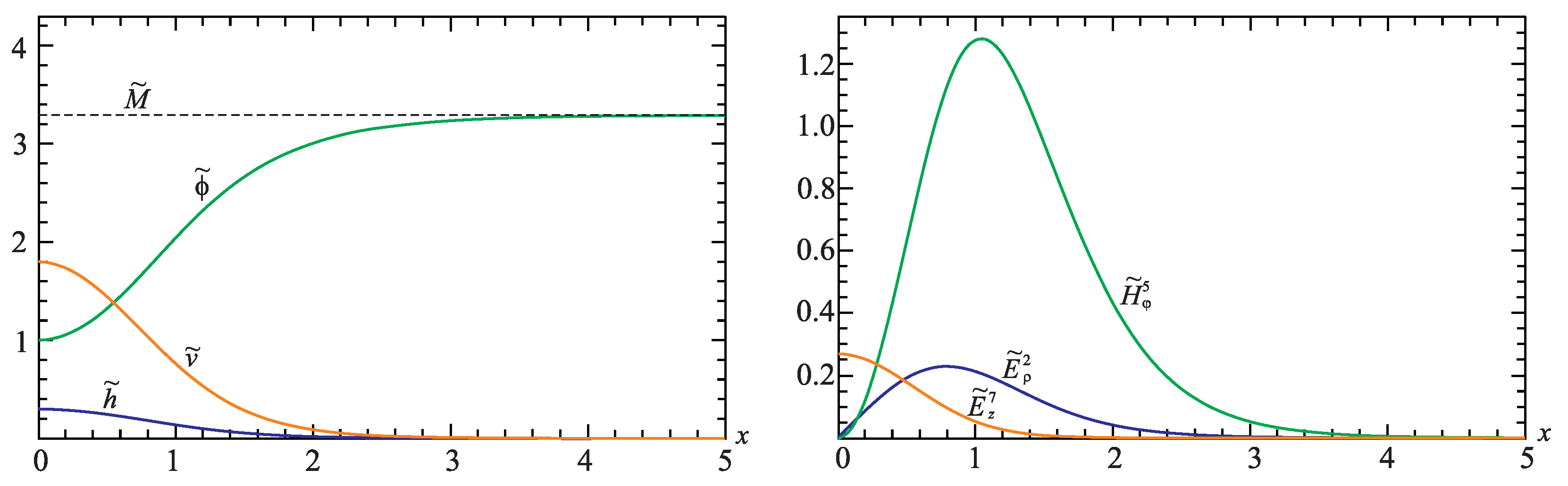
The derivation of solutions to the set of Equations (8)–(10) is an eigenvalue problem for the parameters ${\tilde{\mu }}_1,{\tilde{\mu }}_2$ and $\tilde{M}$. The numerical solution describing the behavior of the Proca field potentials and of the corresponding electric and magnetic fields is given in Figure 1. The behavior of the electric field $E_z^7$ indicates that we are dealing with the dual Meissner effect: this field is pushed out by the scalar field $\varphi$. Notice also that the tube solutions obtained are topologically trivial, in contrast to the Nielsen–Olesen solution.

Let us define the linear energy density $\mathcal{E}$ and the total flux ${\mathsf{\Phi }}_z$ of the longitudinal electric field $E_z^7$ transferred across the cross section of the flux tube as follows:

$$\begin{array}{cc}\hfill \mathcal{E}\equiv \frac{{\varphi }_0^2}{g^2}\tilde{\mathcal{E}}& =2\pi \frac{{\varphi }_0^2}{g^2}\underset{0}{\overset{\infty }{\int }}x\widetilde{ϵ}dx=2\pi {\left(\frac{{\varphi }_0/{\Lambda }_{\mathrm{QCD}}}{g^{\prime }}\right)}^2\hslash c{\Lambda }_{\mathrm{QCD}}^2\underset{0}{\overset{\infty }{\int }}x\widetilde{ϵ}dx,\hfill \end{array}$$

(14)

$$\begin{array}{cc}\hfill {\mathsf{\Phi }}_z\equiv \frac{{\varphi }_0^2}{g^2}{\tilde{\mathsf{\Phi }}}_z& =2\pi \frac{{\varphi }_0^2}{g^2}\underset{0}{\overset{\infty }{\int }}x{\tilde{E}}_z^{7}dx=2\pi {\left(\frac{{\varphi }_0/{\Lambda }_{\mathrm{QCD}}}{g^{\prime }}\right)}^2\hslash c{\Lambda }_{\mathrm{QCD}}^2\underset{0}{\overset{\infty }{\int }}x{\tilde{E}}_z^{7}dx,\hfill \end{array}$$

(15)

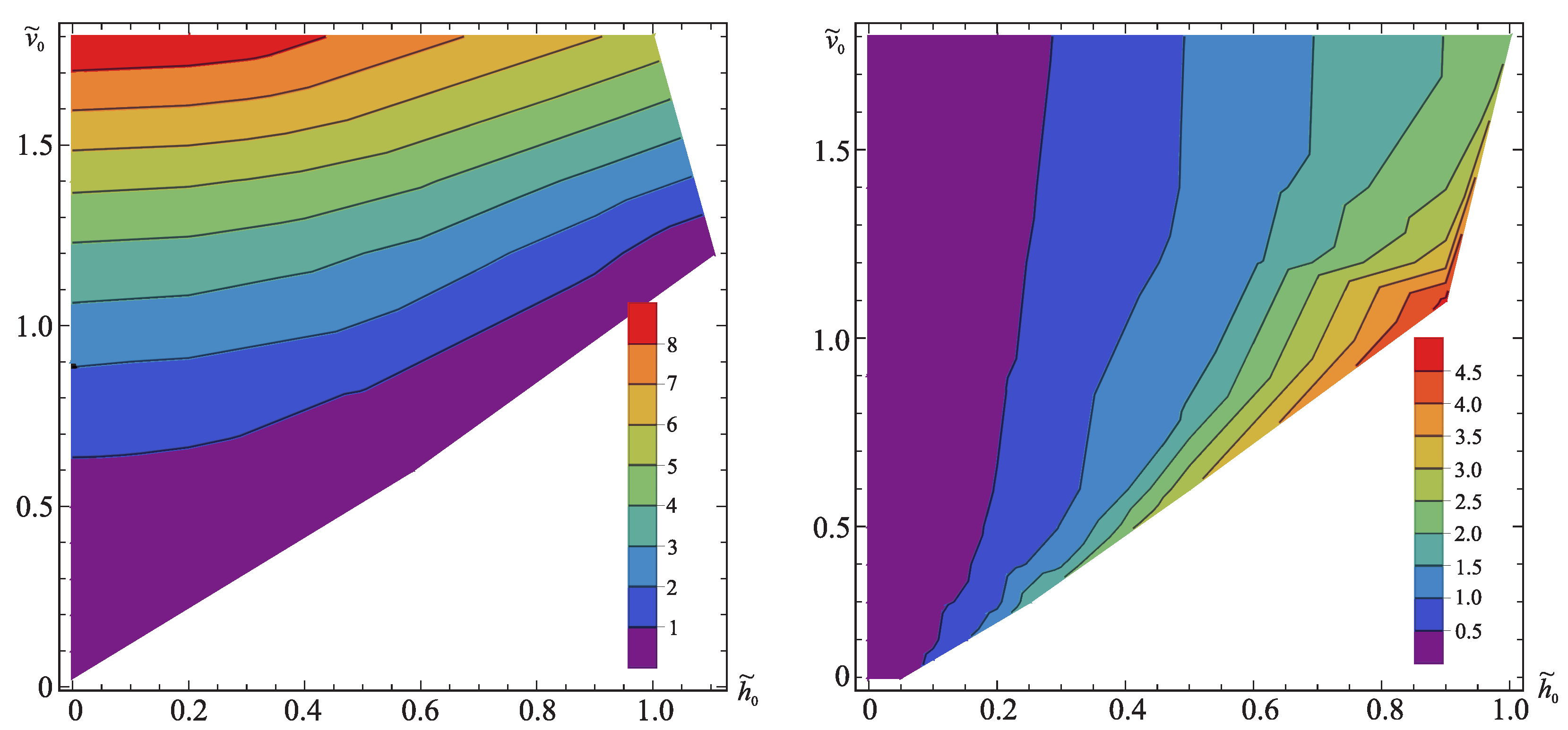
where ${g^{\prime }}^2=g^2\hslash c$ is the dimensionless coupling constant, the tilde sign denotes that the corresponding quantities are dimensionless, and ${\Lambda }_{\mathrm{QCD}}$ is a characteristic parameter coming from QCD. The integral characteristics of these quantities are shown in Figure 2. The analysis of the results shown in Figure 2 suggests the following:

• When $v_0\to 0,h_0=\mathrm{const}$ the linear energy and momentum densities $\tilde{\mathcal{E}}\left(x\right),{\tilde{\mathsf{\Phi }}}_z\left(x\right)\to 0$;
• When $v_0\to \infty ,h_0=\mathrm{const}$ the linear energy and momentum densities $\tilde{\mathcal{E}}\left(x\right),{\tilde{\mathsf{\Phi }}}_z\left(x\right)\to \infty$;
• When $h_0\to 0,v_0=\mathrm{const}$ the linear energy and momentum densities $\tilde{\mathcal{E}}\left(x\right),{\tilde{\mathsf{\Phi }}}_z\left(x\right)\to \mathrm{const}$;
• When $h_0\to \infty ,v_0=\mathrm{const}$ the linear energy and momentum densities $\tilde{\mathcal{E}}\left(x\right),{\tilde{\mathsf{\Phi }}}_z\left(x\right)\to 0$.

Note that, unfortunately, the technical difficulties of numerical solving the set of Equations (8)–(10) do not permit one to study the dependencies $\tilde{\mathcal{E}}\left(x\right)$ and ${\tilde{\mathsf{\Phi }}}_z\left(x\right)$ on the parameters ${\tilde{h}}_0$ and ${\tilde{v}}_0$ in more detail. The reason is that, for small values of ${\tilde{v}}_0$, the calculation accuracy implemented in Wolfram Mathematica does not permit one to find the eigenvalues ${\tilde{\mu }}_{1,2}$ and $\tilde{M}$.

4. Proca Tubes with the Momentum Density

In the previous section, we considered tubes filled with a longitudinal electric field. Such a tube is described by a non-Abelian Proca field sourced by quarks located at $\pm \infty$. In this section, we consider a tube containing nonzero flux of the Poynting vector, whose presence results in the fact that there is an energy flux, and thus the momentum is directed from one source (located at $-\infty$) to another (located at $+\infty$).

For this case, we choose the Ansätze

$$A_t^5=\frac{f\left(\rho \right)}{g},A_z^5=\frac{v\left(\rho \right)}{g},A_{\phi }^7=\frac{\rho w\left(\rho \right)}{g},\varphi =\varphi \left(\rho \right),$$

(16)

which give the following components of the electric and magnetic field intensities:

$$\begin{array}{ccc}\hfill E_{\phi }^2& =& \frac{\rho fw}{2g},E_{\rho }^5=-\frac{f^{\prime }}{g},\hfill \end{array}$$

(17)

$$\begin{array}{ccc}\hfill H_{\rho }^2& =& -\frac{vw}{2g},H_{\phi }^5=-\frac{\rho v^{\prime }}{g},H_z^7=\frac{1}{g}\left(w^{\prime }+\frac{w}{\rho }\right).\hfill \end{array}$$

(18)

In this case, the Poynting vector

$$S^i=\frac{{ϵ}^{ijk}}{\sqrt{\gamma }}{E}_j^a{H}_k^a$$

(19)

is already nonzero (see Equations (31) and (43) below).

Substituting the potentials (16) in Equations (2) and (3) and using the dimensionless variables given before Equation (8), we derive the following equations:

$$\begin{array}{ccc}\hfill {\tilde{f}}^{″}+\frac{{\tilde{f}}^{\prime }}{x}& =& \tilde{f}\left(\frac{{\tilde{w}}^2}{4}+{\tilde{\varphi }}^2-{\tilde{\mu }}_1^2\right),\hfill \end{array}$$

(20)

$$\begin{array}{ccc}\hfill {\tilde{v}}^{″}+\frac{{\tilde{v}}^{\prime }}{x}& =& \tilde{v}\left(\frac{{\tilde{w}}^2}{4}+{\tilde{\varphi }}^2-{\tilde{\mu }}_2^2\right),\hfill \end{array}$$

(21)

$$\begin{array}{ccc}\hfill {\tilde{w}}^{″}+\frac{{\tilde{w}}^{\prime }}{x}-\frac{\tilde{w}}{x^2}& =& \tilde{w}\left(-\frac{{\tilde{f}}^2}{4}+\frac{{\tilde{v}}^2}{4}+{\tilde{\varphi }}^2-{\tilde{\mu }}_3^2\right),\hfill \end{array}$$

(22)

$$\begin{array}{ccc}\hfill {\tilde{\varphi }}^{″}+\frac{{\tilde{\varphi }}^{\prime }}{x}& =& \tilde{\varphi }\left[\tilde{\lambda }\left(-{\tilde{f}}^2+{\tilde{v}}^2+{\tilde{w}}^2\right)+\tilde{\Lambda }\left({\tilde{\varphi }}^2-{\tilde{M}}^2\right)\right],\hfill \end{array}$$

(23)

where $\tilde{f}=f/{\varphi }_0$, $\tilde{w}=w/{\varphi }_0$, and we have introduced the component of the Proca field mass matrix ${\mu }_3^2={\left({\mu }^2\right)}_{\phantom{ab,}\phi }^{77,\phi }$. This set of equations has a cylindrically symmetric solution describing a tube with nonzero momentum density and energy flux (the Poynting vector).

Our purpose is to study the dependence of the linear momentum density $\int \overrightarrow{S}d\overrightarrow{\sigma }$ on the boundary conditions ${\tilde{f}}_0,{\tilde{v}}_0,{\tilde{w}}_0$ given at the center and the parameter $\tilde{\Lambda }$. Unfortunately, the number of these parameters is too large to investigate this dependence in detail; our goal is therefore to reduce this number. To do this, in the next subsection, we examine the case with $\tilde{w}=0$. Such a restriction results in the fact that we actually deal with Proca electrodynamics; i.e., with $U\left(1\right)$ massive electrodynamics possessing the $U\left(1\right)$ group spanned on the ${\lambda }_5$ Gell–Mann matrix.

4.1. Abelian Proca Tubes

Consider the simplest case in which the component of the potential $A_{\phi }^7=0$. In this case, we deal with massive (Proca) electrodynamics.

Let us examine the simplest particular case where $\tilde{f}=hsinh\xi ,\tilde{v}=hcosh\xi$ with $\xi =\mathrm{const}.$ and ${\tilde{\mu }}_1={\tilde{\mu }}_2=\tilde{\mu }$. In this case the set of Equations (20)–(23) is split as follows. Equation (20) takes the form of the Schrödinger equation,

$$-h^{″}-\frac{h^{\prime }}{x}+h{\tilde{\varphi }}^2={\tilde{\mu }}^{2}h,$$

(24)

where the function ${\tilde{\varphi }}^2$ plays the role of the effective potential for the “wave function” h. In order to ensure a regular solution of this equation, it is necessary for the effective potential to have a well. In this case, Equation (24) must be solved as an eigenvalue problem for the parameter ${\tilde{\mu }}^2$ with the eigenfunction h.

The remaining Equation (23) for the function $\tilde{\varphi }$ is then

$${\tilde{\varphi }}^{″}+\frac{{\tilde{\varphi }}^{\prime }}{x}=\tilde{\varphi }\left[\tilde{\lambda }{h}^2+\tilde{\Lambda }\left({\tilde{\varphi }}^2-{\tilde{M}}^2\right)\right].$$

(25)

Introducing new variables $\overline{x}=x\tilde{\lambda }$ and $\overline{\varphi }=\tilde{\varphi }/\sqrt{\tilde{\lambda }}$ and the constants $\overline{\mu }=\tilde{\mu }/\sqrt{\tilde{\lambda }},\overline{M}=\tilde{M}/\sqrt{\tilde{\lambda }}$, Equations (24) and (25) can be recast in the form

$$\begin{array}{cc}\hfill -h^{″}-\frac{h^{\prime }}{\overline{x}}+{\overline{\varphi }}^{2}h=& {\overline{\mu }}^{2}h,\hfill \end{array}$$

(26)

$$\begin{array}{cc}\hfill {\overline{\varphi }}^{″}+\frac{{\overline{\varphi }}^{\prime }}{\overline{x}}=& \overline{\varphi }\left[h^2+\tilde{\Lambda }\left({\overline{\varphi }}^2-{\overline{M}}^2\right)\right],\hfill \end{array}$$

(27)

where the prime denotes differentiation with respect to $\overline{x}$.

We seek regular solutions with a finite linear energy density. This means that, asymptotically (as $\overline{x}\to \infty$), the function $h\left(\overline{x}\right)\to 0$. Then, taking into account the positiveness of the effective potential ${\overline{\varphi }}^2$, one can conclude that the function $\overline{\varphi }$ must go to a constant, and Equation (27) implies that this constant is $\overline{M}$; i.e., $\overline{\varphi }\to \overline{M}\mathrm{as}\overline{x}\to \infty$.

We seek solutions for Equations (26) and (27), which in the vicinity of the origin of coordinates have the form

$$\begin{array}{cc}\hfill h\left(\overline{x}\right)=& h_0+h_2\frac{{\overline{x}}^2}{2}+\dots \mathrm{with}{h}_2=\frac{h_0}{2}\left({\overline{\varphi }}_0^2-{\overline{\mu }}^2\right),\hfill \end{array}$$

(28)

$$\begin{array}{cc}\hfill \overline{\varphi }\left(\overline{x}\right)=& {\overline{\varphi }}_0+{\overline{\varphi }}_2\frac{{\overline{x}}^2}{2}+\dots \mathrm{with}{\overline{\varphi }}_2=\frac{{\overline{\varphi }}_0}{2}\left[h_0^2+\tilde{\Lambda }\left({\overline{\varphi }}_0^2-{\overline{M}}^2\right)\right],\hfill \end{array}$$

(29)

where the expansion coefficients $h_0$ and ${\overline{\varphi }}_0$ are arbitrary.

In turn, the asymptotic behavior of the functions is

$$h\left(\overline{x}\right)\approx h_{\infty }\frac{e^{-\overline{x}\sqrt{{\overline{M}}^2-{\overline{\mu }}^2}}}{\sqrt{\overline{x}}},\overline{\varphi }\left(\overline{x}\right)\approx \overline{M}-{\overline{\varphi }}_{\infty }\frac{e^{-\overline{x}\sqrt{2\tilde{\Lambda }{\overline{M}}^2}}}{\sqrt{\overline{x}}},$$

where $h_{\infty }$ and ${\overline{\varphi }}_{\infty }$ are integration constants.

The typical profiles of the potential $h\left(\overline{x}\right)$ and of the scalar $\overline{\varphi }\left(\overline{x}\right)$, obtained numerically, are shown in Figure 3. Furthermore, this figure shows the corresponding graph for the dimensionless energy density

$$\begin{array}{c}\hfill \begin{array}{cc}\hfill \overline{\epsilon }\equiv \frac{g^6}{{\lambda }^2{\varphi }_0^4}\epsilon =& \frac{{sinh}^2\xi +{cosh}^2\xi }{2}{\left(h^{\prime }\right)}^2+\frac{{\left({\overline{\varphi }}^{\prime }\right)}^2}{2}-\frac{{\overline{\mu }}^2\left({sinh}^2\xi +{cosh}^2\xi \right)}{2}{h}^2\hfill \\ \hfill & +\frac{{\overline{\mu }}^2\left({sinh}^2\xi +{cosh}^2\xi \right)}{2}{\overline{\varphi }}^2{h}^2+\frac{\tilde{\Lambda }}{4}{\left({\overline{\varphi }}^2-{\overline{M}}^2\right)}^2.\hfill \end{array}\end{array}$$

(30)

The substitution of the components of electric and magnetic fields (17) and (18) in Equation (19) yields the following expression for the Poynting vector:

$$S^z=\frac{1}{g^2}\frac{df}{d\rho }\frac{dv}{d\rho }=\frac{{\lambda }^2{\varphi }_0^4}{g^6}sinh\xi cosh\xi {\left(h^{\prime }\right)}^2=\frac{{\lambda }^2{\varphi }_0^4}{g^6}{\overline{S}}^z={\lambda }^2\left(\frac{{\varphi }_0^4/{\Lambda }_{\mathrm{QCD}}^4}{g^{\prime 6}}\right){\hslash }^3{c}^3{\Lambda }_{\mathrm{QCD}}^4{\overline{S}}^z,$$

(31)

whose typical behavior is given in Figure 3. Note that the presence of the gradient terms $f^{\prime }$ and $v^{\prime }$ means (as already shown above) that we are dealing with massive Proca electrodynamics.

In our study, the integral characteristics are of great interest. Namely, these are the linear energy density,

$$\overline{\mathcal{E}}=\frac{g^2}{{\varphi }_0^2}\mathcal{E}=2\pi \underset{0}{\overset{\infty }{\int }}\overline{x}\overline{\epsilon }d\overline{x}$$

(32)

and the linear momentum density across the cross section of the tube,

$${\overline{\Pi }}^z=\frac{g^2}{{\varphi }_0^2}{M}^z=2\pi \underset{0}{\overset{\infty }{\int }}\overline{x}\overline{S^z}d\overline{x}$$

(33)

shown in Figure 4 as functions of the parameters $h_0$ and $\tilde{\Lambda }$. The numerical calculations indicate that both these integral characteristics depend weakly on the coupling constant $\tilde{\Lambda }$.

Thus, we have shown in this subsection that, in Proca electrodynamics, there can exist tubes filled with constant electric and magnetic fields creating the energy flux (or, equivalently, the momentum) directed along the tube axis. This situation differs in principle from the case in an electromagnetic wave, where the energy flux (and the momentum) is created by time-dependent electric and magnetic fields. The existence of such a tube possessing energy flux and momentum depends in principle on the presence of the Higgs scalar field.

Based on the analysis of numerical solutions of the corresponding equations, we can suppose that

• the linear energy, $\mathcal{E}$, and momentum, ${\Pi }^z$, densities depend weakly on the coupling constant of the Higgs scalar field $\Lambda$;
• when $h_0\to 0$ the quantities $\mathcal{E},{\Pi }^z\to 0$;
• when $h_0\to \infty$ the quantities $\mathcal{E},{\Pi }^z\to \infty$.

4.2. Non-Abelian Proca Tubes

Consider the case of $\tilde{f}=\tilde{v},\tilde{w}\ne 0$ and ${\tilde{\mu }}_1={\tilde{\mu }}_2=\tilde{\mu }$. In this case, the set of Equations (20)–(23) is split as follows. Equation (20) takes the form of the Schrödinger equation,

$$-{\tilde{f}}^{″}-\frac{{\tilde{f}}^{\prime }}{x}+\tilde{f}{U}_{\tilde{f},\mathrm{eff}}={\tilde{\mu }}^2\tilde{f},$$

(34)

where the effective potential for the “wave function” $\tilde{f}$ is

$$U_{\tilde{f},\mathrm{eff}}=\frac{{\tilde{w}}^2}{4}+{\tilde{\varphi }}^2.$$

(35)

As in the previous subsection, Equation (34) must be solved as an eigenvalue problem for the parameter ${\tilde{\mu }}^2$ with the eigenfunction $\tilde{f}$.

The remaining Equations (22) and (23) for the functions $\tilde{w}$ and $\tilde{\varphi }$ are then

$$\begin{array}{ccc}\hfill -{\tilde{w}}^{″}-\frac{{\tilde{w}}^{\prime }}{x}+\tilde{w}{U}_{\tilde{w},\mathrm{eff}}& =& {\tilde{\mu }}_3^2\tilde{w},\hfill \end{array}$$

(36)

$$\begin{array}{ccc}\hfill {\tilde{\varphi }}^{″}+\frac{{\tilde{\varphi }}^{\prime }}{x}& =& \tilde{\varphi }\left[\tilde{\lambda }{\tilde{w}}^2+\tilde{\Lambda }\left({\tilde{\varphi }}^2-{\tilde{M}}^2\right)\right],\hfill \end{array}$$

(37)

and they do not already contain the function $\tilde{f}$. The effective potential, which appears in Equation (36), is

$$U_{\tilde{w},\mathrm{eff}}=\frac{1}{x^2}+{\tilde{\varphi }}^2.$$

(38)

The Equation (36) has the form of the Schrödinger equation with the “wave function” $\tilde{w}$ and with the “energy” ${\tilde{\mu }}_3^2$. This means that it will have a regular solution only if the effective potential $U_{\tilde{w},\mathrm{eff}}$ possesses a well.

We seek solutions of Equations (34), (36), and (37), which in the vicinity of the origin of coordinates have the form

$$\begin{array}{ccc}\hfill \tilde{f}\left(x\right)& =& {\tilde{f}}_0+{\tilde{f}}_2\frac{x^2}{2}+\dots \mathrm{with}{\tilde{f}}_2=\frac{{\tilde{f}}_0}{2}\left({\tilde{\varphi }}_0^2-{\tilde{\mu }}^2\right),\hfill \end{array}$$

(39)

$$\begin{array}{ccc}\hfill \tilde{w}\left(x\right)& =& {\tilde{w}}_{1}x+{\tilde{w}}_3\frac{x^3}{3!}+\dots \mathrm{with}{\tilde{w}}_3=\frac{2}{3}{\tilde{w}}_1\left({\tilde{\varphi }}_0^2-{\tilde{\mu }}_3^2\right),\hfill \end{array}$$

(40)

$$\begin{array}{ccc}\hfill \tilde{\varphi }\left(x\right)& =& {\tilde{\varphi }}_0+{\tilde{\varphi }}_2\frac{x^2}{2}+\dots \mathrm{with}{\tilde{\varphi }}_2=\frac{{\tilde{\varphi }}_0}{2}\tilde{\Lambda }\left({\tilde{\varphi }}_0^2-{\tilde{M}}^2\right),\hfill \end{array}$$

(41)

where the expansion coefficients ${\tilde{f}}_0,{\tilde{\varphi }}_0$, and ${\tilde{w}}_1$ are arbitrary.

In turn, the asymptotic behavior of the functions is

$$\tilde{f}\left(x\right)=\tilde{v}\left(x\right)\approx {\tilde{f}}_{\infty }\frac{e^{-x\sqrt{{\tilde{M}}^2-{\tilde{\mu }}^2}}}{\sqrt{x}},\tilde{w}\left(x\right)\approx {\tilde{w}}_{\infty }\frac{e^{-x\sqrt{{\tilde{M}}^2-{\tilde{\mu }}_3^2}}}{\sqrt{x}},\tilde{\varphi }\approx \tilde{M}-{\tilde{\varphi }}_{\infty }\frac{e^{-x\sqrt{2\tilde{\Lambda }{\tilde{M}}^2}}}{\sqrt{x}},$$

where ${\tilde{f}}_{\infty },{\tilde{w}}_{\infty }$, and ${\tilde{\varphi }}_{\infty }$ are integration constants.

The typical profiles of the functions $\tilde{f}\left(x\right),\tilde{w}\left(x\right)$, and $\tilde{\varphi }\left(x\right)$ and of the dimensionless energy density

$$\begin{array}{c}\hfill \begin{array}{cc}\hfill \tilde{\epsilon }\equiv \frac{g^2}{{\varphi }_0^4}\epsilon =& \frac{{\left({\tilde{f}}^{\prime }\right)}^2}{2}+\frac{{\left({\tilde{v}}^{\prime }\right)}^2}{2}+\frac{1}{2}{\left({\tilde{w}}^{\prime }+\frac{\tilde{w}}{x}\right)}^2+\frac{1}{\tilde{\lambda }}\frac{{\left({\tilde{\varphi }}^{\prime }\right)}^2}{2}+\frac{{\tilde{w}}^2}{8}\left({\tilde{f}}^2+{\tilde{v}}^2\right)\hfill \\ \hfill & -\frac{{\tilde{\mu }}_1^2}{2}{\tilde{f}}^2-\frac{{\tilde{\mu }}_2^2}{2}{\tilde{v}}^2-\frac{{\tilde{\mu }}_3^2}{2}{\tilde{w}}^2+\frac{{\tilde{\varphi }}^2}{2}\left({\tilde{f}}^2+{\tilde{v}}^2+{\tilde{w}}^2\right)+\frac{\tilde{\Lambda }}{4\tilde{\lambda }}{\left({\tilde{\varphi }}^2-{\tilde{M}}^2\right)}^2\hfill \end{array}\end{array}$$

(42)

are shown in Figure 5. The substitution of the components of electric and magnetic fields (17) and (18) in Equation (19) yields the following expression for the Poynting vector:

$$S^z=\frac{1}{g^2}\left(\frac{df}{d\rho }\frac{dv}{d\rho }+\frac{1}{4}fv{w}^2\right)=\frac{{\varphi }_0^4}{g^2}\left({\tilde{f}}^{\prime }{\tilde{v}}^{\prime }+\frac{1}{4}\tilde{f}\tilde{v}{\tilde{w}}^2\right)=\frac{{\varphi }_0^4}{g^2}{\tilde{S}}^z=\left(\frac{{\varphi }_0^4/{\Lambda }_{\mathrm{QCD}}^4}{g^{\prime 2}}\right)\hslash c{\Lambda }_{\mathrm{QCD}}^4{\tilde{S}}^z,$$

(43)

whose distribution is given in Figure 5. Note that this expression contains the gradient term ${\tilde{f}}^{\prime }{\tilde{v}}^{\prime }$ (which is the same as that given in Equation (31)) and the nonlinear term $\tilde{f}\tilde{v}{\tilde{w}}^2/4$, which appears because the Proca field is non-Abelian.

Similarly to Section 4.1, we have calculated the integral characteristics of the non-Abelian tube filled with the color electric and magnetic Proca fields. The results are given in Figure 6.

Thus, we have shown in this subsection that in SU(3) non-Abelian Proca theory, there exist tubes filled with stationary, crossed color electric and magnetic fields, which, by virtue of being crossed, create the energy flux and momentum directed along the tube axis. These solutions are topologically trivial.

The analysis of the results obtained permits us to assume that

• the linear momentum density ${\Pi }^z$ depends weakly on $w_1$, which is the value of the potential $A_{\phi }^7$ on the tube axis;
• the linear energy density $\mathcal{E}\to \mathrm{const}$ for $f_0\to 0,w_1=\mathrm{const}$;
• the linear momentum density ${\Pi }^z\to 0$ for $f_0\to 0,w_1=\mathrm{const}$;
• $\mathcal{E},{\Pi }^z\to \infty$ as $w_1\to \infty$.

5. Conclusions

In the present paper, we continued our investigations that we began in [4,5] concerning tube solutions within SU(3) non-Abelian–Proca–Higgs theory. Our purpose was to obtain the integral characteristics of those solutions. We were interested in obtaining the dependencies of the flux of the longitudinal electric field and linear momentum/energy densities on the system parameters.

We have considered two types of tubes. For tubes of the first type, possessing the flux of the longitudinal color electric field, we have obtained the dependencies of the flux and of the linear energy density on the value of the coupling constant $\Lambda$ and on the values of the fields at the center of the tube. For the tubes of the second type, possessing momentum density, we have found the dependencies of the linear momentum and energy densities on the values of the fields at the center of the tube.

The results obtained can be summarized as follows:

• For the tube with the flux of a color electric Proca field directed along the tube axis, we have studied the dependence of the linear energy density and of the flux of such a field on the values of the components $A_t^2$ and $A_z^5$ on the tube axis;
• For the tube with the energy flux (and thus with the momentum directed along the tube axis), we have examined the dependence of the linear energy and momentum densities on the values of the components $A_{t,z}^5$ and $A_{\phi }^7$ on the tube axis;
• The existence of the aforementioned tube solutions depends crucially on the presence of the Higgs scalar field singlet (there are no such solutions without this field);
• The tube solutions obtained are topologically trivial, in contrast to the Nielsen–Olesen solution [1] carrying a topological charge;
• The solution with the color longitudinal electric field demonstrates the dual Meissner effect: the electric field is pushed out by the Higgs scalar field.

QCD is SU(3) non-Abelian Yang–Mills theory containing one dimensional constant ${\Lambda }_{\mathrm{QCD}}=200\mathrm{MeV}/\hslash c\approx 1{\mathrm{fm}}^{-1}\approx {10}^{13} {\mathrm{cm}}^{-1}$. Here, we have considered SU(3) non-Abelian Proca theory, which differs from QCD by having massive terms. It is seen from the corresponding formulae that all the integral characteristics calculated here depend on ${\varphi }_0$, whose dimension is $\left[{\varphi }_0\right]={\mathrm{cm}}^{-1}$. For this reason, it is interesting to estimate the values of the integral quantities under consideration for ${\varphi }_0\approx {\Lambda }_{\mathrm{QCD}}$. In this case, the dimensional coefficients appearing in the expressions (14) and (15) are

$${\left(\frac{{\varphi }_0/{\Lambda }_{\mathrm{QCD}}}{g^{\prime }}\right)}^2\hslash c{\Lambda }_{\mathrm{QCD}}^2\approx 200\mathrm{MeV}/\mathrm{fm}\approx 3.2·{10}^9\mathrm{erg}/\mathrm{cm}\approx 3\mathrm{tones};$$

the latter value is of the same order as the force of interaction between quarks, which appears as a consequence of the existence of a flux tube filled with a SU(3) gauge Yang–Mills field and connecting the quarks.

In conclusion, we would like to state that, in order to understand the nature of confinement in QCD, it is necessary to have flux tubes filled with a color longitudinal electric field that connect quarks and create a linear potential between quarks ensuring confinement. Another interesting feature of QCD is that gluon fields give a considerable contribution to the proton spin. As we demonstrated in [4,5] and in the present paper, in SU(3) non-Abelian Proca theory, there are two types of tube solutions: (i) those with the flux of color electric field (in Proca theory, where such tubes connect “quarks” and may lead to confinement in massive Yang-Mills theories); (ii) those with the momentum directed along the tube (if such tubes connect “quarks” in a Proca proton, they will contribute to the Proca proton spin). This means that massive non-Abelian Yang–Mills theories (non-Abelian Proca theories) have some similarities to quantum chromodynamics; this gives a good reason for the detailed study of such theories. One more motivation for studying cylindrical solutions supported by massive vector fields might be the possibility of using them for the modeling of such gravitating configurations as cosmic strings both within Einstein’s gravity [8] and in various modified gravities [9].

References

- Nielsen, H.B.; Olesen, P. Vortex Line Models for Dual Strings. Nucl. Phys. B 1973, 61, 45–61. [Google Scholar] [CrossRef]
- Brihaye, Y.J.; Verbin, Y. Superconducting and spinning non-Abelian flux tubes. Phys. Rev. D 2008, 77, 105019. [Google Scholar] [CrossRef] [Green Version]
- Brihaye, Y.J.; Verbin, Y. Proca Q Tubes and their Coupling to Gravity. Phys. Rev. D 2017, 95, 044027. [Google Scholar] [CrossRef] [Green Version]
- Dzhunushaliev, V.; Folomeev, V. Proca tubes with the flux of the longitudinal chromoelectric field and the energy flux/momentum density. Eur. Phys. J. C 2020, 80, 1043. [Google Scholar] [CrossRef]
- Dzhunushaliev, V.; Folomeev, V.; Kozhamkulov, T.; Makhmudov, A.; Ramazanov, T. Non-Abelian Proca theories with extra fields: Particlelike and flux tube solutions. Phys. Scripta 2020, 95, 074013. [Google Scholar] [CrossRef]
- Obukhov, Y.N. Analog of black string in the Yang-Mills gauge theory. Int. J. Theor. Phys. 1998, 37, 1455. [Google Scholar] [CrossRef]
- Singleton, D. Axially symmetric solutions for SU(2) Yang-Mills theory. J. Math. Phys. 1996, 37, 4574. [Google Scholar] [CrossRef] [Green Version]
- Vilenkin, A.; Shellard, E.P.S. Cosmic Strings and Other Topological Defects, 2nd ed.; Cambridge University Press: Cambridge, MA, USA, 2000. [Google Scholar]
- Nojiri, S.; Odintsov, S.D.; Oikonomou, V.K. Modified Gravity Theories on a Nutshell: Inflation, Bounce and Late-time Evolution. Phys. Rep. 2017, 692, 1–104. [Google Scholar] [CrossRef] [Green Version]
Figure 1.
The typical profiles of the functions , and and of the dimensionless fields , , and for , , , .
Figure 2.
The contour profiles of the dimensionless linear energy density (left panel) and of the dimensionless flux of the longitudinal electric field (right panel) as functions of the parameters and for the tube with the flux of the longitudinal electric field.
Figure 3.
The typical profiles of the functions and and of the dimensionless energy density and dimensionless momentum density for , , , .
Figure 4.
The contour profiles of the dependence of the linear energy density (left panel) and of the linear momentum density (right panel) on the parameters and .
Figure 5.
The typical profiles of the functions , , the dimensionless energy and the momentum density for , , .
Figure 6.
The contour profiles of the linear energy density (left panel) and of the linear momentum density (right panel) on the parameters and .
Publisher’s Note: MDPI stays neutral with regard to jurisdictional claims in published maps and institutional affiliations. |
© 2021 by the authors. Licensee MDPI, Basel, Switzerland. This article is an open access article distributed under the terms and conditions of the Creative Commons Attribution (CC BY) license (https://creativecommons.org/licenses/by/4.0/).
Share and Cite
MDPI and ACS Style
Dzhunushaliev, V.; Folomeev, V.; Tlemisov, A. Linear Energy Density and the Flux of an Electric Field in Proca Tubes. Symmetry 2021, 13, 640. https://doi.org/10.3390/sym13040640
AMA Style
Dzhunushaliev V, Folomeev V, Tlemisov A. Linear Energy Density and the Flux of an Electric Field in Proca Tubes. Symmetry. 2021; 13(4):640. https://doi.org/10.3390/sym13040640
Chicago/Turabian StyleDzhunushaliev, Vladimir, Vladimir Folomeev, and Abylaikhan Tlemisov. 2021. "Linear Energy Density and the Flux of an Electric Field in Proca Tubes" Symmetry 13, no. 4: 640. https://doi.org/10.3390/sym13040640
Note that from the first issue of 2016, this journal uses article numbers instead of page numbers. See further details here.