Severity Classification of Diabetic Retinopathy Using an Ensemble Learning Algorithm through Analyzing Retinal Images

Abstract

Diabetic Retinopathy (DR) refers to the damages endured by the retina as an effect of diabetes. DR has become a severe health concern worldwide, as the number of diabetes patients is soaring uncountably. Periodic eye examination allows doctors to detect DR in patients at an early stage to initiate proper treatments. Advancements in artificial intelligence and camera technology have allowed us to automate the diagnosis of DR, which can benefit millions of patients indeed. This paper inscribes a novel method for DR diagnosis based on the gray-level intensity and texture features extracted from fundus images using a decision tree-based ensemble learning technique. This study primarily works with the Asia Pacific Tele-Ophthalmology Society 2019 Blindness Detection (APTOS 2019 BD) dataset. We undertook several steps to curate its contents to make them more suitable for machine learning applications. Our approach incorporates several image processing techniques, two feature extraction techniques, and one feature selection technique, which results in a classification accuracy of 94.20% (margin of error: ±0.32%) and an F-measure of 93.51% (margin of error: ±0.5%). Several other parameters regarding the proposed method’s performance have been presented to manifest its robustness and reliability. Details on each employed technique have been included to make the provided results reproducible. This method can be a valuable tool for mass retinal screening to detect DR, thus drastically reducing the rate of vision loss attributed to it.

1. Introduction

Diabetes mellitus (diabetes) collectively refers to a group of metabolic disorders that occurs if a person has an elevated sugar level in his/her blood and does not produce sufficient insulin to regulate it. Diabetes has become a severe health problem all over the world in the last few decades. According to the International Diabetes Federation (IDF) reports, globally, 463 million people between 20 and 79 had diabetes in 2019 [1]. Based on their predictions, the number will reach an overwhelming 700 million by 2045. The World Health Organization (WHO) reported a 5% increase in premature mortality from diabetes since 2000 [2]. Among the four primary types of diabetes, type 1 and type 2 diabetes are chronic, whereas genetic deficits and gestational diabetes are reversible in most cases [3]. Diabetes causes numerous health complications, including vision impairment due to Diabetic Retinopathy (DR), heart attacks, kidney failure, and stroke. DR results from the vandalization of the blood vessels within the retina’s tissue caused by prolonged diabetes. Consequently, blood, fluids, and lipids enter inside the macula and block the person’s vision. DR patients often experience impaired color vision, blurred vision, loss of central vision, floaters within the vision space, and poor eyesight at night. At the advanced stages of DR, patients experience total blindness, and in most cases, the condition becomes permanent.

In the US, the number of cases of DR surged 89%, from 4.06 million to 7.69 million, within ten years (2000–2010) [4]. According to their projections, the number of DR cases will reach 14 million by 2050. DR is the leading cause of vision impairment among people younger than 74 years [5]. The number of diabetes cases is increasing worldwide, and it is becoming increasingly hard to diagnose DR among all the patients. The primary reason is that the disease shows almost no symptoms at its earlier stages [5]. The only way to detect DR at these stages is to get regular eye checkups. However, with the growing number of diabetes cases, ensuring that all patients get regular checkups is very difficult, even for a developed country such as the US; according to a 2017 report, 21.4% of diabetes cases in the US went undiagnosed [6]. Globally, the rate of undiagnosed diabetes cases is an alarming 50% (232 million people) [1]. The traditional (manual) DR diagnostic systems are already inadequate to provide diagnoses to all diabetes patients. With the number of type 2 diabetes patients increasing in most countries, these manual diagnostic systems’ capacity is merely insufficient to meet the requirement for constant checkups of all diabetes patients. That is the reason we need to look for alternative ways for DR diagnosis. With proper treatment initiated at the right time, more than 90% of the DR patients can recover their eyesight or prevent the disease from being vision-threatening [7].

Recent advancements in machine learning and artificial intelligence have imparted a far-reaching impact on numerous science and engineering fields. Clinical diagnosis is one of those fields that have benefited the most because of these developments. New and improved machine learning algorithms allowed researchers to automate the diagnosis of many diseases. Researchers have been trying to do the same for DR diagnosis as well. So far, several powerful methods have been proposed and practiced in this regard. Practical DR diagnosis is made based on retinal images collected using a procedure called Fundus Photography. These images capture the retina and its contents with vivid details. Convolutional Neural Network (CNN) based state-of-the-art methods work very well on clean DR images. The existing DR identification approaches differ in many aspects, including the source of the retinal images, methods of image pre-processing, type of the features extracted from retinal images, and the utilized machine learning algorithm. Most researchers use deep learning methods to work with retinal image datasets. Notably, CNN-based deep learning methods are very popular in this regard, and they are often handy. In the last 19 years, more than 425 articles have been published in renowned journals outlining various methods for DR detection [8]. We present some of the notable works of recent times using deep learning algorithms in the following few paragraphs.

In 2020, D. Hemanth et al. proposed a Deep Convolutional Neural Network (DCNN)-based DR detection and classification method [9]. They used contrast-limited adaptive histogram equalization (CLAHE) and histogram equalization imaging techniques and acquired a classification accuracy of 97% and an F-measure of 94%. K. Shankar et al. reported a synergic deep learning model for DR classification incorporating both the image processing and segmentation techniques [10]. They tested their method on the Messidor dataset and obtained over 99% classification accuracy. Gayathri et al. used a CNN model with six convolutional layers and two fully connected layers to extract features from fundus photographs [11]. Then, the authors used several classifiers, including Support Vector Machine (SVM), Multilayer Perceptron, Random Forest (RF), and J48 to classify the samples of several datasets. Their proposed method acquired near-perfect classification outcomes in many cases. Liu et al. proposed three hybrid model structures based on CNN and an improved loss function (enhance cross-entropy) for DR classification in their 2020 article [12]. They used five different popular deep learning architectures: EfficientNetB4, InceptionResNetV2, EfficientNetB5, NASNetLarge, and Xception as the base of their proposed method and trained three hybrid models on the outputs of these methods. The resultant method registered 86.34% classification accuracy and 98.77% sensitivity on the EyePACS dataset. Shankar et al. introduced a Hyperparameter Tuning Inception-v4 (HPTI-v4) model to classify DR images [13]. They used CLAHE for image pre-processing and a histogram-based segmentation model for segmenting color fundus images. They acquired a peak accuracy of 96.25% on the Messidor dataset. Li proposed a Cross-disease Attention Network (CANet) for grading DR and Diabetic Macular Edema [14]. In their study, the authors designed two attention modules: a disease-specific module that utilizes both the inter-spatial and inter-channel relationship among the features and a disease-dependent module that exploits the inter-channel features collected from the retinal images. They tested their method on two public datasets (ISBI 2018 IDRiD challenge and Messidor) and obtained 85.10% joined classification accuracy.

In 2019, Li et al. described a four-class (three non-prolific DR and one prolific DR) classification algorithm based on a customized DCNN architecture [15]. In their study, they replaced the conventional max-pooling layers with fractional max-pooling layers. Their study involved 34,124 retinal images collected from a Kaggle competition dataset. However, their model scored an 86.17% classification accuracy making it somewhat convenient for practical use. Bellemo et al. proposed a CNN-based DR classification method trained using the Singapore National Diabetes Retinopathy Screening Program (SIDRP) dataset containing 76,370 retinal images [15] and validated their methods using another 4504 images collected from urban centers in the Copperbelt province of Zambia. Although they did not mention the accuracy, they provided the sensitivity and specificity values of their model, which are 92.25% and 89.04%, respectively. Sayres et al. used the popular EyePACS dataset, which contains 140,000 retinal images, to build a deep learning model [16]. The primary purpose of their study was to understand the impact of DR-classification algorithms on physician readers in computer-assisted settings. They recorded an 88.40% classification accuracy with both the sensitivity and specificity scores over the 90th percentile. Zeng et al. proposed a Binocular Siamese-like CNN-based method employing 28,104 selected images from the EyePACS dataset [17]. However, with 82.2% sensitivity and just 70.70% specificity, it can be said that their model did not register a reliable performance. Zhang et al. narrated an automatic DR detection and grading system following the Grading Scale of Diabetic Retinopathy (GSDR) [18]. They used 3062 DR images in the training phase and performed external validation afterward. Their model has high sensitivity and specificity scores, both over 97%. de la Torre et al. proposed a CNN-based pixel-wise score-propagation model retaining 76,650 images from the EyePACS dataset [19]. The specialty of their model lies in the architecture of the CNN; for every neuron, it divides the observed output score into two separate components. However, questions can be asked about the method’s performance, as it renders sensitivity and specificity scores around 91% and does not go through any external validation. Pires et al. developed a multi-class DR-classification method sequentially employing multiple CNNs using 88,702 retinal images collected from two Kaggle competition datasets [20]. They kept the trade-off between efficiency and effectiveness in mind while building the model, which makes it particularly suitable for implementing in smartphones.

Although non-deep learning-based DR detection methods are not so standard, they are not rare. In 2013, Akram et al. proposed a classification technique using the Gaussian Mixture Model and SVM [21]. In 2014, Antal and Hajdu described a two-class (binary) DR-detection method incorporating several Decision Tree (DT)-based classifiers [22]. In 2014, Wang et al. outlined an approach combining a CNN model with RF for blood vessel segmentation inside the retina [23]. In 2016, Mane and Jadhav proposed a holoentropy-enabled DT for DR identification [24]. They tested their method on DIARETDB0 and DIARETDB1 fundus image databases and acquired 96.45% classification accuracy. In 2017, Saleh et al. proposed a DR assessment method using a fuzzy RF along with a dominance-based rough set balanced rule [25]. In 2019, Jebaseeli et al. described a deep learning-based SVM (DLBSVM) for DR categorization [26]. They procured 201 fundus images from five different datasets and obtained near-perfect classification performance on them.

Retinal images may contain a magnitude of noise and interference if collected using non-standard equipment and in non-ideal environments, which is often the case. This study deals with such a set of noisy retinal images collected from a reasonably new DR dataset. We employed several steps to suppress the effects of noise present in the samples. We calculated the histogram and Gray Level Co-occurrence Matrix (GLCM) of these images and used them as statistical features extracted from the samples. Then, we identified the most important features using a popular feature selection method named Genetic Algorithm (GA). We used those features to train a robust ensemble learning algorithm called Extreme Gradient Boosting (XGBoost). The proposed method resolves a multi-class classification problem, which corresponds to DR’s severity in the associated retinal images. The XGBoost algorithm was hyper-tuned to obtain the best performance on this particular application. The acquired results proclaim that the proposed approach can successfully categorize the dataset samples. We provide necessary tables, figures, and graphs while describing its steps and performance for proper interpretation.

The rest of the paper is organized as follows. Section 2 discusses the employed dataset and its contents, cites the prior works involving it, outlines the study’s methodology, and describes the image processing and classification techniques used in this study. Section 3 presents the obtained classification results and justifies their reliability. Finally, Section 4 provides concluding remarks on the paper, an overview of the entire article, and mentions some scopes for further research.

2. Materials and Methods

This study’s workflow can be partitioned into four main sets of operations: retinal image collection, image pre-processing, feature extraction and selection, and DR model creation and optimization. We employed multiple image processing techniques to pre-process the retinal images, extract features from them, and a DT-based ensemble method known as XGBoost for image classification. The entire workflow has been presented in Figure 1 and narrated elaborately in the following subsections.

2.1. Employed Dataset and Prior Works on It

This study used the fundus images contained by the Asia Pacific Tele-Ophthalmology Society 2019 Blindness Detection (APTOS 2019 BD) dataset [27]. This image dataset contains 3662 samples collected from many participants of rural India. Aravind Eye Hospital, India, organized the dataset. The hospital technicians traveled to India’s remote areas to collect the retinal image samples using fundus photography. These fundus photographs were collected in varying conditions and environments over a long period. Later, a group of trained doctors reviewed and labeled the gathered samples following the principle of the International Clinical Diabetic Retinopathy Disease Severity Scale (ICDRSS). As per the scaling system, the APTOS 2019 BD samples are divided into five categories: no DR, mild DR, moderate DR, severe DR, and proliferative DR. The first category encompasses the healthy retinal samples where no DR is present. Each of the latter categories represents slightly more damaged retinas than the previous one. The last class, proliferative DR, is comprised of the samples that contain vitreous or pre-retinal hemorrhage. Sample retinal images of all the classes have been presented in Appendix A.

Although not the first of its kind, APTOS 2019 BD is an adequate dataset to work with, and it has received quite the reception among researchers and data science experts. More than 2900 teams participated in the associated Kaggle competition, and since its emergence last year, around 20 research articles have been published (so far). We present a brief discussion on the existing body of works involving this dataset in the following few paragraphs.

In 2019, K. Singh and D. Drzewicki described a classification method using a pre-trained VGG-19 network [28]. However, in their study, they used the Limited-memory Broyden–Fletcher–Goldfarb–Shanno (L-BFGS) algorithm instead of the famous Adam optimizer and claimed that it led to cleaner results. S. Kassani et al. reported a method where they used four deep learning architectures—InceptionV3, MobileNet, ResNet50, and Xception to extract features from the dataset’s images [29]. Dekhil et al. adopted a transfer learning approach and classified the dataset’s samples using the ImageNet architecture, which was previously trained on 3.2 million images [30]. Sikder et al. presented a method incorporating the ExtraTree classifier, which is a popular ensemble learning algorithm [31]. Their paper used several image processing techniques to pre-process the retinal images and extracted histogram features from them.

In 2020, Wang and Schaefer of Stanford University, California, US, described a classification method using a pre-trained MobileNetV2 architecture [32]. They used data augmentation and a weighted loss function to classify the APTOS 2019 BD dataset’s images. Sheikh presented a thesis using three deep learning models—DenseNet121, VGG16, and MobileNetV2 for DR classification [33]. The author achieved the best classification outcome using MobileNetV2 architecture. Sheikh and Qidwai outlined a smartphone-based DR severity detection method [34]. Their study used four CNN-based methods—DenseNet121, VGG16, RestNet50, and InceptionV3—for DR classification. The authors experimented with and without employing image pre-processing techniques. As expected, they achieved their peak performance when the images were pre-processed. Pak et al. performed multiple classifications on the dataset samples with various deep learning architectures such as DenseNet121, ResNet50, ResNet101, and EfficientNet-b4. They achieved the highest accuracy using EfficientNet-b4 [35]. Gangwar and Ravi presented a Transfer Learning-based deep learning algorithm where they classified the images of this dataset with a pre-trained Inception-ResNet-v2 [36]. They added a custom block of CNN to make it a hybrid model and tested this model on the Messidor-1 dataset as well.

Bodapati et al. proposed a multi-modal fusion module using pre-trained ConvNet models for DR classification [37]. They performed two separate tasks—DR detection (binary classification) and determining its severity (multi-class classification). They also reported that a dropout at the input layer of a Deep Neural Network converges quicker while trained with blended features instead of uni-modal deep features. Kueterman described a classifier with a two-stage CNN architecture and SVM feature extraction for DR classification in a thesis work [38]. Patel and Chaware presented a Transfer Learning-based Fine-tuned MobileNetV2 architecture [39]. They experimented with customized and fine-tuned models with a varying number of epochs in their research. Liu et al. proposed a Graph REsidual rE-ranking Network (GREEN) in their reported work for DR classification based on the APTOS 2019 BD dataset [40]. The EfficientNet-b0 architecture is the backbone of their described method. Dondeti et al. extracted deep features from the fundus images of the dataset and used ⱱ-Support Vector Machine (ⱱ-SVM) for DR classification [41]. They extracted deep features using the Neural Architecture Search Network (NASNet) architecture. Zhuang and Ettehadi used a modified Efficientnet-B3 architecture for DR classification [42]. They also experimented with a shallow learning method in their study. Still, they acquired better results using the previous architecture.

Table 1. DR classification performance comparison on the Asia Pacific Tele-Ophthalmology Society 2019 Blindness Detection (APTOS 2019 BD) dataset.

Reference	Classification Method	Accuracy (%)	Precision (%)	Recall (%)	Specificity (%)	F-Measure (%)
[28]	Pre-trained VGG-19	82.70	43.00	62.00	–	50.78
[29]	InceptionV3, MobileNet, ResNet50, and Xception	83.09	–	88.24	87.00	–
[30]	ImageNet (transfer learning)	77.00	–	–	–	–
[31]	ExtraTree	91.07	90.40	89.54	–	89.97
[32]	MobileNetV2	78.47	68.66	60.01	–	64.04
[33]	MobileNetV2	91.68	77.64	83.17	80.11	80.31
[34]	DenseNet121	90.50	93.00	90.00	87.00	88.47
[35]	EfficientNet-b4	79.00	–	–	–	–
[36]	Hybrid Inception ResNet-v2 (transfer learning)	82.18	–	–	–	–
[37]	Pre-trained ConvNet	80.96	80	81	–	80
[38]	ResNet50 + SVM	82.40	≈63	≈71	≈95	≈66
[39]	Tuned MobileNetV2	81.63	–	–	–	–
[40]	EfficientNet-b0 + GREEN	81.60	–	–	–	78.20
[41]	ⱱ-SVM	77.90	75.00	77.00	–	76.50
[42]	Modified Efficientnet-B3	77.87	–	–	–	–
Proposed (All features)	Tuned XGBoost	94.20	94.34	92.68	96.44	93.51
Proposed (Selected features)	Tuned XGBoost	93.70	93.06	91.71		92.38

If multiple classifications were performed in the study, the best results were taken. “–“ indicates that the score was not reported in the corresponding article/study.

compares the reported results acquired by the classification methods applied to the APTOS 2019 BD dataset by the previously cited studies. As the table shows, CNN-based deep learning architectures did not show excellent results. Our research experimented with numerous deep learning models to reach a higher and more reliable classification outcome. However, this approach did not provide results significantly better than the existing methods. Therefore, we decided to work with manually extracted features and tree-based algorithms. After working with many sets of features and a few variants of bagging and boosting techniques, we reached the classification model described in the following section.

2.2. Pre-Processing of the Employed Dataset

Retinal images contained by the APTOS 2019 BD dataset are very convenient. The dataset has many noisy images, duplicate images labeled as different classes, images of various resolutions, and varying sample sizes. Before moving on to the feature extraction and learning stages, these issues need to be resolved or minimized to build a successful DR classification model. Below, we describe how we dealt with these challenges in this study.

2.2.1. Dealing with Excessively Noisy Images

The dataset contains several images with a high degree of noise and interference. All the images of the dataset were checked manually to single out the most affected ones. Those images were excluded from this study. We excluded samples in this study through visual inspection. A total of 566 images were discarded due to containing artifacts or being too underexposed, overexposed, or out of focus. Other reasons for exclusion include chromatic aberrations, digitization error, image saturation, blur, dust, darkness, and lens condensation. A few retinal images excluded from this study have been presented in Appendix A. Such sample exclusion was also performed by authors of the studies [43,44] They reported that this initial step is advantageous for efficient training and inference on the image dataset.

2.2.2. Dealing with Duplicate Images

The dataset contains quite a few duplicate samples, most of which have been marked with different class labels. This kind of noise in labeling makes the learning model prone to misclassification. We calculated the similarities between every two images based on their two-dimensional (2D) correlation coefficients to find such occurrences. The basic idea behind calculating the 2D correlation coefficient is to determine how much two matrices are similar to each other in a quantitative manner [45]. If we have two sample grayscale images, $I_A^r$ and $I_B^r$, their 2D correlation coefficient can be determined using:

$$corr\left(I_A^r,I_B^r\right)= \frac{{{\displaystyle \sum }}_m{{\displaystyle \sum }}_n(I_A^r{}_{mn}-\overline{I_A^r})(I_B^r{}_{mn}-\overline{I_B^r})}{\sqrt{\left[{{\displaystyle \sum }}_m{{\displaystyle \sum }}_n{\left(I_A^r{}_{mn}-\overline{I_A^r}\right)}^2\right]\left[{{\displaystyle \sum }}_m{{\displaystyle \sum }}_n{\left(I_B^r{}_{mn}-\overline{I_B^r}\right)}^2\right]}}$$

(1)

where $\overline{I_A^r}$ and $\overline{I_B^r}$ are the mean of all values of the matrices $I_A^r$ and $I_B^r$, respectively [46]. Equation (1) always results in a value within 0 and 1; 0 if $I_A^r$ and $I_B^r$ are nothing alike, and 1 if they are the same. Since we are working with color (RGB) images, we had to calculate the coefficients separately for three different channels. If the outcomes of all the three channels are 1, then we can conclude that the second image is a copy of the first one. Suppose we want to calculate the coefficients between every two images of the 3096 images (remaining after noisy image exclusion). In that case, the operation has to be repeated ³⁰⁹⁶C₂ times, which would take a long time to perform and may seem unreasonable. Therefore, we first checked if the resolution (height and width in pixels) of two images match to reduce the number of operations. The 2D correlation coefficients of the two images were calculated only if the images had the same resolution. The whole process of duplicate image checking is summarized in Algorithm 1. Correlations of all three channels were checked for extra precision. We primarily focused on finding the exact images/files marked as different classes (possibly by different graders) with this algorithm. However, duplicates may exist in images of different sizes as well. Since the total number of samples was not very high, removing too many samples could have made the model less reliable. Using Algorithm 1, we found duplicates of 115 retinal images within the remaining 3096 images (after the previous step). In most cases, the copies of a sample have different class labels. We randomly picked one of the duplicate images and discarded the other(s). The rest of the study was conducted with the remaining 2981 retinal images.

Algorithm 1: An algorithm to detect duplicate images of the same size
Input Output	: :	Two-color images, $I_A$ and $I_B$. A decision on whether or not $I_B$ is a duplicate of $I_A$. 0 → $I_B$ is not a duplicate of $I_A$ 1 → $I_B$ is a duplicate of $I_A$
Step-1	:	Determine the resolution of $I_A$ and $I_B$: $res\left(I_A\right)\leftarrow$ height & width of $I_A$ (in pixel). $res\left(I_B\right)\leftarrow$ height & width of $I_B$ (in pixel). if $res\left(I_A\right)$ == $res\left(I_B\right)$  Determine $corr\left(I_A,I_B\right)$ using Equation (1) for three channels. else  return 0
Step-2	:	if$corr\left(I_A,I_B\right)$==1 for all three channels  return 1 else  return 0

2.2.3. Dealing with Unwanted Black Borders

The majority of the images of the APTOS 2019 BD dataset contain black pixels close to the borders. As these pixels do not carry any information on DR’s existence in the associated retinal image, a simple image crop operation can remove them. We summarize the process in Algorithm 2. This operation is relatively straightforward for the images that contain the entire eyeball inside its frame, such as Figure 2a. However, most of the images (such as Figure 2c) have part of the retina missing (from top and bottom), which is also another drawback of the dataset. In these cases, black pixels were only removed from the left and right sides to prevent further loss of useful information (from inside the eyeball). This step is helpful, since we will extract histogram features from the images later on. Figure 2b,d show the resultant images of the crop operation applied on the images of Figure 2a,c, respectively.

Algorithm 2: An algorithm for image crop
Input Output	: :	A retinal image, $I_A$ A cropped image without black borders, $I_A^{\prime }$
Step-1	:	Determine the resolution of $I_A$ and $I_B$. $\left(h,w\right)\leftarrow$ height & width of $I_A$ (in pixel).
Step-2	:	Determine the center pixel of the image: $C_h\leftarrow floor\left(h/2\right)$; $C_w\leftarrow floor\left(w/2\right)$
Step-3	:	Identify the first non-black pixel directly above the center pixel: for $i=1$ to $h$  if $\left(i, C_w\right)$ > 10 in all three channels   $C_1\leftarrow i$; break directly left to the center pixel: for $i=1$ to $w$  if $\left(C_h,i\right)$ > 10 in all three channels   $C_3\leftarrow i$; break	directly below the center pixel: for $i=h$ to $1$  if $\left(i, C_w\right)$ > 10 in all three channels   $C_2\leftarrow i$; break directly right to the center pixel: for $i=w$ to $1$  if $\left(C_h,i\right)$ > 10 in all three channels   $C_4\leftarrow i$; break
Step-4	:	Crop the image: for $i=1$ to $3$  $I_A^{\prime }\left(:,:i\right)\leftarrow I_A\left(C_1:C_2, C_3:C_4, i\right)$
Step-5	:	return$I_A^{\prime }$

2.2.4. Dealing with Uneven Image Resolution

As mentioned before, the APTOS 2019 BD dataset images have varying resolutions, ranging from 474 × 358 to 3388 × 2588 pixels in width and height, respectively. This dissimilarity can be an issue for our further processing. Therefore, we performed an image resize operation to rescale all the images to 256 × 256 pixels in this step. The images that do not contain the entire eyeball (such as Figure 3a) will be compressed along its width, as shown in Figure 3b. This step might seem unideal, but we allowed this compression since we aimed to maintain a uniform square shape and did not want to lose further information from the images.

2.2.5. Dealing with Uneven Sample Sizes

Table 2. The number (and percentage) of images of each class remaining after various steps of the workflow.

DR Severity	Class ID	Dataset	After Noisy and Duplicate Image Exclusion		After Augmentation
No DR	NO	1875	1406	47.17%	1406	26.60%
Mild DR	MI	370	308	10.33%	1232	23.31%
Moderate DR	MO	999	807	27.07%	807	15.27%
Severe DR	SE	193	185	6.20%	740	14.00%
Prolific DR	PR	295	275	9.23%	1100	20.82%
Total		3662	2981	100%	5285	100%

presents the number of images of five different classes present in the APTOS 2019 BD dataset. As seen from the table, the dataset is imbalanced, or in other words, the associated classes do not have the same number of samples. The issue persists after removing the excessively noisy images and duplicate images. At this point, the sample size of the NO class (the majority class) is almost eight times larger than that of the Severe DR (SE) class (the minority class). Compared to No DR (NO), Mild DR (MI) and Prolific DR (PR) have significantly smaller sample sizes as well. There are several disadvantages to working with such an imbalanced dataset. Bias in decisions toward the majority class while judging new samples is the most acute one. To deal with this problem, we augmented the existing samples of the MI, SE, and PR classes to create new samples. Each image of the mentioned classes was rotated by 90$°$, 180$°$, and 270$°$ to obtain sample sizes four times larger than the previous ones. As shown in Table 2, this operation does not solve the issue entirely but reduces it to some extent. After augmentation, we have 5285 retinal images, where 26.60% of the samples belong to the majority class and 14% belong to the minority class.

2.2.6. Increasing the Sharpness of the Images

As mentioned earlier, the dataset images contain noise and interference. Many of the images are partially blurry or hazy, making it more challenging to mine distinguishable features from them. One way to deal with this issue is to increase the sharpness of the images, emphasizing their texture by making the borders among different regions more apparent. This study used unsharp masking, a well-known image sharpening method, to enhance the retinal images’ sharpness. The main idea behind unsharp masking is to subtract a blurred version of the retinal image from the original one to detect its edges. Then, a mask is constructed with the acquired edge details. Finally, the contrast is increased at the edges, and the effect is applied to the original image. If we take a sample image, $I_A$, its sharpened form $I_S$ can be calculated as follows [47]:

$$I_S\left(h,h\right)=I_A\left(h,h\right)+\lambda \nabla \left(h,h\right)$$

(2)

Here, $h$ is the height and width of the image in pixels (since we have square-shaped images from the image resize operation), $\lambda$ is a factor that adjusts the intensity of sharpening, and $\nabla \left(h,h\right)$ is a suitably-defined gradient at $\left(h,h\right)$ [48]. One of the widely used gradient functions is the discrete Laplacian operator [49], which can be defined as follows:

$$\nabla \left(h,h\right)\triangleq I_A\left(h,h\right)-\frac{1}{4}\left[I_A\left(h-1,h\right)+I_A\left(h,h-1\right)+I_A\left(h+1,h\right)+I_A\left(h,h+1\right)\right].$$

(3)

We can get $I_S$ using Equations (2) and (3). The resultant image is shaped by three parameters of the operation—amount, radius, and threshold. Amount refers to the intensity of sharpness. Radius governs the area around the edges that are affected by the sharpening operation. A large value of the radius will sharpen a wider region around the edges, and a smaller value will do so to a narrower region. Threshold allows the algorithm to decide if a pixel will be considered an edge pixel and reduces the sharpening noise. In this study, we used [2, 1, 0.1] as the value of the amount, radius, and threshold, respectively. Figure 4b shows a sample retinal image (Figure 4a) sharpened using the unsharp masking technique.

2.2.7. Image Pre-Processing

We employed one more image processing technique to pre-process the retinal images before extracting features from the resultant sharpened images. We used Tone mapping, which is an imaging technique widely used in digital cameras, at this step. Tone mapping transforms a high dynamic range image into a low dynamic range image. Digital cameras use this operation to make the captured images more suitable for digital displays. However, we used this technique to compress the dynamic range of the retinal images and preserve the crucial information within them, such as local contrast, global contrast, details, etc., at the same time. Each tone of the original image is mapped to achieve a tone suitable for viewing. Tone mapping is carried out on a three-channel image ($I_A$) using an operator defined as follows:

$$𝓉\left(I_A\right)={ℝ}_i^{h\times w\times 3}\to {\mathbb{D}}_O^{h\times w\times 3}$$

(4)

where ${ℝ}_i\subseteq ℝ$, ${\mathbb{D}}_O\subset {ℝ}_i$, and ${\mathbb{D}}_O=\left[0,255\right]$ [50]. Tone mapping changes the luminance information of the original image while leaving the color information preserved. Equation (4) can be simplified as follows:

$$𝓉\left(I_A\right)=\{\begin{array}{c}{L}_d=t\left(H_d\right) : {ℝ}_i^{h\times w}\\ \left[\begin{array}{c}{R}_L\\ G_L\\ B_L\end{array}\right]=L_d{\left(\frac{1}{H_d}\left[\begin{array}{c}{R}_H\\ G_H\\ B_H\end{array}\right]\right)}^{𝓈}\end{array}$$

(5)

where $L_d$ and $H_d$ are the low dynamic range and high dynamic range luminance values of a pixel, respectively. $𝓈\in \left(0,1\right]$ is called the saturation factor. $R_L, G_L,$ and $B_L$ are the low dynamic ranges of red, green, and blue channels; and $R_H, G_H,$ and $B_H$ are the high dynamic ranges of red, green, and blue channels, respectively. In this study, the global tone mapping system was used, where all the pixels are mapped with the same value of $𝓉$. In the local tone mapping system, the mapping of each pixel depends on its neighboring pixels. $𝓉$ can be applied to each pixel of a retinal image in three different ways: linear scaling, exponential mapping, and logarithmic mapping [50]. In linear scaling, the main image is multiplied by a factor $𝕖$, which is defined as follows:

$$L_d{\left(p_i\right)}_{linear}=𝕖H_d\left(p_i\right)$$

(6)

where $p_i$ is a sample pixel. For logarithmic mapping and exponential mapping, the relationships between $L_d$ and $H_d$ are defined in Equations (7) and (8), respectively.

$$L_d{\left(p_i\right)}_{logarithmic}=\frac{{\log }_{10}\left(1+k_1{H}_d\left(p_i\right)\right)}{{\log }_{10}\left(1+k_2{H}_d{\left(p_i\right)}_{max}\right)}$$

(7)

$$L_d{\left(p_i\right)}_{exponential}=1-\exp \left(-\frac{k_1{H}_d\left(p_i\right)}{k_2{H}_d{\left(p_i\right)}_{mean}}\right)$$

(8)

where $k_1\in \left(1,\infty \right]$ and $k_2\in \left[\infty ,1\right)$ are two constants. Although their outcomes are visibly similar, we used the exponential mapping operation to approximate the retinal images’ appearance in this study. Figure 4c presents a tone-mapped outlook of the image shown in Figure 4b.

2.3. Feature Set Creation

With the retinal images’ pre-processing, we can now move on to the next step of the workflow: feature extraction. Figure 5 shows the tree channels’ information of a sample processed retinal image. As seen from the figure, most of the blue channel pixels are black or near-black, indicating very little distinguishable information useful for the learning algorithm. The color images’ blue channel can be omitted to lessen the number of features. However, as we plan to use a feature selection algorithm, later on, we are keeping the channel and the features extracted from it for now. We extracted two sets of features from each retinal image: histogram and GLCM. Below, we describe these two widely used imaging techniques.

2.3.1. Histogram Feature Extraction

The histogram of an image portrays the relative frequency of occurrence of the varying gray levels in that image [49]. If we consider the range of the gray labels, a sample gray label image is ($0$ to $l-1$), which can be expressed as a discrete function as follows:

$$𝓅\left(g_k\right)=\frac{n_k}{h\times w}$$

(9)

where $g_k$ is the $k$-th gray label, $n_k$ is the number of pixels with that particular gray label, and $h\times w$ is the number of total pixels of the image [51]. Since we are working with 8-bit color images, in our case, the range of the gray labels is from 0 to 255. Figure 6 provides a histogram plot (not-normalized) of the image’s three channels presented in Figure 5a. As seen from the figure, most of the blue channel pixels reside within the gray labels ranging from 0 to 50, whereas the red and green channels contain a wide range of gray labels.

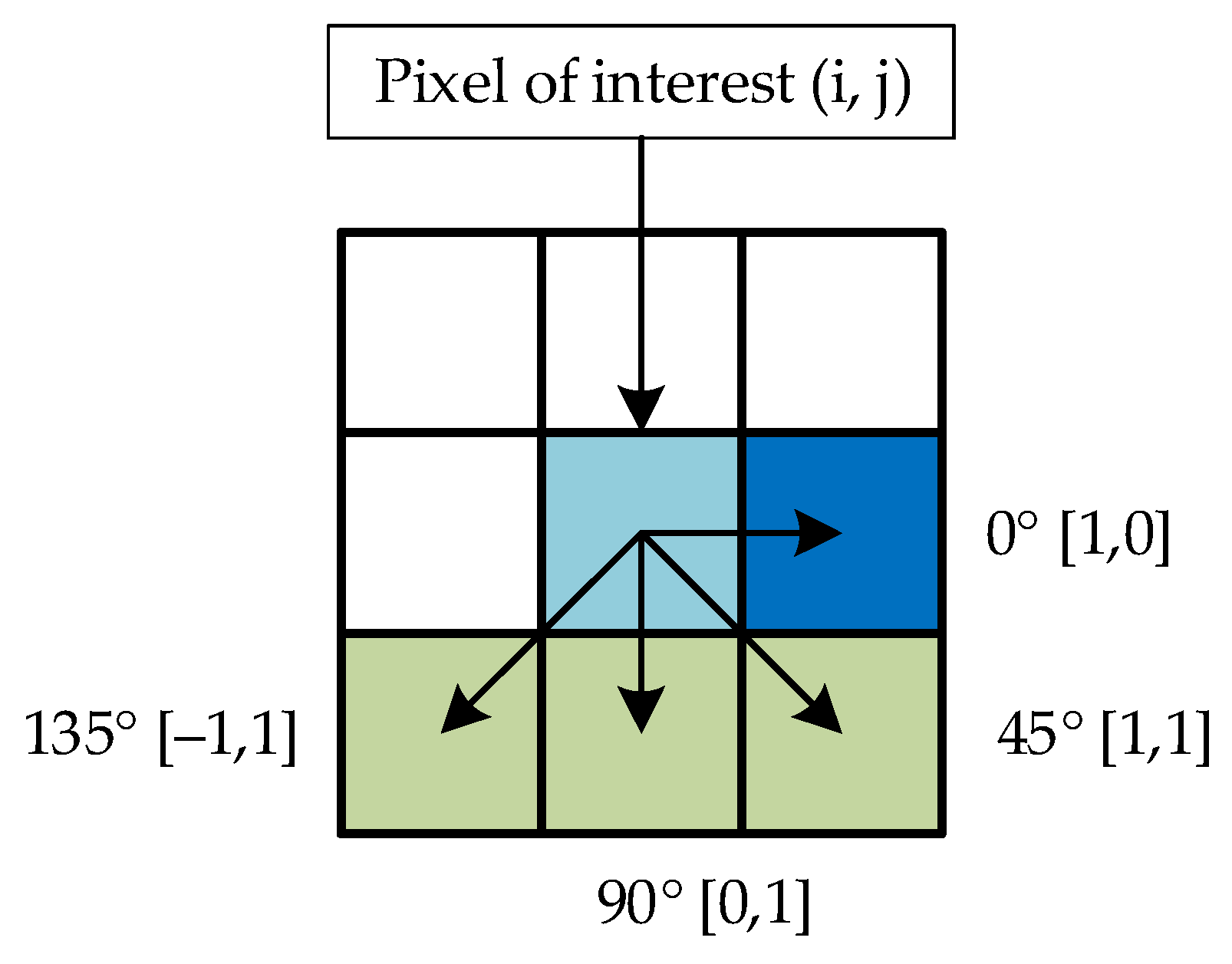
2.3.2. Gray-Level Co-Occurrence Information Extraction

GLCM primarily highlights the texture information of an image. It can be expressed as a matrix function of the distance and angle between neighboring pixels. Haralick et al. worked extensively with different variants of GLCM of an image and other parameters that can be derived from it in the 1970s [52,53]. The GLCM of a grayscale image is a measure of the frequencies at which different combinations of gray levels or pixel values occur in that image [54]. We are working with 256 pixels $\times$ 256 pixels retinal images, where the value of each pixel lies in the range of 0–255. First, to calculate the GLCM of such an image, its pixel values are rescaled to distinct levels 1–8. The values can also be scaled to other or more discrete levels if necessary. However, in this study, levels 1–8 were used. This newly formed matrix is called a Scaled image ($S$). GLCM expresses how often a pixel value ($k$) occurs either diagonally, horizontally, or vertically to another pixel value ($l$). The co-occurrence matrix (${\mathcal{C}}_m$) of the image is specified with a displacement vector $d=\left\{\left(row, column\right)\right\}$ shown in Figure 7. ${\mathcal{C}}_m\left(k,l\right)$ points out how many times a $k$ is separated from $l$ by the displacement vector. Therefore, ${\mathcal{C}}_m\left(k,l\right)$ can be defined as follows:

$${\mathcal{C}}_m\left(k,l\right)={{\displaystyle \sum }}_{k=1}^8{{\displaystyle \sum }}_{l=1}^8\{\begin{array}{l}1, if S\left(i,j\right)=k and\\ S\left(i\pm d, j\pm d\right)=l\\ 0, otherwise\end{array}.$$

(10)

The resultant matrix is an 8 $\times$ 8 matrix containing the frequencies of different combinations of $\left(k,l\right)$ in $S$ [55]. In this study, we chose to work with the $0° \left[1,0\right]$ displacement vector shown in Figure 7. Figure 8 shows the GLCM of the retinal image shown in Figure 5a.

2.3.3. Feature Concatenation

The above-described feature extraction techniques were applied to each channel of the retinal images. Histogram features calculated from the three channels were concatenated, which resulted in 768 features in total. GLCM features derived from each channel were flattened to consider them as a row vector of 64 features. Three GLCMs from three channels result in a total of 192 features. Combining these two sets of features, we obtained a set of 960 features extracted from a single retinal image. The process was repeated for all the 5285 samples to acquire the complete set of features used in this study.

2.3.4. Selection of the Most Relevant Features

The dimension of the training data is a crucial factor in machine learning. Although high-dimensional data contain more information about the corresponding sample, the samples become sparser and far apart from the other samples of the same class in a high-dimensional space, making it harder for learning algorithms to set decision boundaries. This phenomenon is known as the curse of dimensionality, and it has a profound effect on the performance of any machine learning algorithm [56]. Feature selection methods offer a simple solution to this problem by identifying the most important features and omitting the rest. Various feature selection methods are available that work based on different principles. In this study, we choose to work with a DT-based GA. GAs are evolutionary algorithms; they work with candidate solutions and gradually evolve toward better outcomes [57]. GAs are inherently inspired by the process of natural selection and have gotten most of their terminology from that branch of biology.

A typical GA starts with several random guesses, which is known as a population. The population usually spreads throughout the entire search space. A basic GA performs three primary operations to direct the population—selection, crossover, and mutation [58]. A GA aims to converge toward the global optimum over a series of steps, which are known as generations. As the names suggest, these operators’ functionalities are similar to the process of natural selection. Selection attempts to pressurize the population members so that better-performing or “fitter” members are propagated toward the next generation, and weaker members are thrown out of the pool. This phenomenon strengthens the performance of the population of the next generation. Crossover allows multiple possible solutions to exchange information among them and create numerous subsets of new solutions, some of which might be better than the initial solutions. Mutation randomly alters values to see if that changes the outcome positively. Since this may cause radical changes in the outcome, the amount of mutation is typically kept very low. A new population emerges as a result of applying these operators to the previous population. This generation is again modified by the operators and propagated toward the next generation. This process is repeated until a predefined number of generations have elapsed or a certain criterion of convergence has been met, or if the solution remains unchanged for a certain number of generations. Algorithm 3 describes the working procedure of a basic GA [59].

Algorithm 3: Steps of feature selection using basic GA
Input Output	: :	A set of features and labels, $𝓧=<x_1,y_1>, \dots <x_n,y_n>$ Fitness function, 𝒻 (∙,∙) Fitness threshold, $\tau$ Population size, $p_s$ A set of strong (the fittest) features
Step-1	:	population of $p_s$ random individuals, $P_0$
Step-2	:	for$k$ = $0$ to $\infty$  sum$\leftarrow 0$   Compute the fitness of the population:   for each individual $j\in P_k$    sum $\leftarrow$ sum + $𝒻\left(j,𝓧\right)$     if $𝒻\left(j,𝓧\right)\ge \tau$      return $j$   Compute the selection probabilities:   for each individual $j\in P_k$    $P{r}_k\left[j\right]$ $\leftarrow 𝒻\left(j,𝓧\right)/sum$   Select and breed:   for $i = 1$ to $p_s/2$    select $j_1, j_2\in P_k$ based on $P{r}_k$    $j_1, j_2\leftarrow$ crossover$\left(j_1, j_2\right)$    $j_1\leftarrow$ mutate$\left(j_1\right)$    $j_2\leftarrow$ mutate$\left(j_2\right)$    $P_{k+1}\leftarrow P_{k+1}+\left\{j_1, j_2\right\}$

2.4. DR Image Classification

XGBoost is a DT-based ensemble learning algorithm used for solving both classification and regression problems. XGBoost falls into the category of boosting algorithms as it improves its prediction power by training a set of weak learners and gradually converting them into strong ones. It was developed by Chen and Guestrin in 2014; XGBoost is an improvement upon the basic Gradient Boosting algorithm [60]. There are quite a few advantages to using XGBoost. First of all, it is faster than the other boosting methods, since it builds trees parallelly, whereas the other boosting methods build trees sequentially, thus learning from the data at slower rates. Secondly, XGBoost has a built-in regularization technique to minimize overfitting [61]. Thirdly, it uses an approximation algorithm that speeds up the model training process. Lastly, XGBoost can efficiently handle weighted and sparse data and supports out-of-core computing. As a result of these reasons, XGBoost has become a commonly used DT-based supervised learning algorithm. To describe how XGBoost works, let us consider a dataset, $D=\left\{\left(x_i, y_i\right)\right\}$ such that $\left|D\right|=n, x_i\in {ℝ}^m,$ and $y_i\in {ℝ}^n$ which has $m$ features and $n$ examples. The model output of a boosting algorithm with $T$ trees is defined as follows:

$${\widehat{y}}_i={\displaystyle \sum }_{t=1}^T{f}_k\left(x_i\right), f_t\in ℱ$$

(11)

where $ℱ=\left\{f\left(x\right)={\omega }_{𝓆}\left(x\right)\right\}$ is a set of trees built to solve a classification task [62]. Each $f_t$ divides a tree into two parts: leaf weight part ($\omega$) and structure part ($𝓆$). $f_t$ can be learned by minimizing the following objective function:

$$\mathcal{O}={{\displaystyle \sum }}_i\ell ({\widehat{y}}_i,y_i)+{{\displaystyle \sum }}_t\mathsf{\Omega }(f_t).$$

(12)

Here, $\ell$ is a training loss function measuring the distance between ${\widehat{y}}_i$ and $y_i$, which are the prediction and the object, respectively. $\mathsf{\Omega }$ represents the penalty of the model complexity. Traditional optimization methods cannot optimize a boosting algorithm with the objective function expressed in Equation (12) in Euclidean space. In the Gradient Boosting algorithm, the prediction and the objective function of the $k$-th iteration are defined as follows:

$${\widehat{y}}^{\left(k\right)}={\widehat{y}}^{\left(k-1\right)}+f_k\left(x\right)$$

(13)

$${\mathcal{O}}^{\left(k\right)}={{\displaystyle \sum }}_{i=1}^n\ell \left(y_i,{\widehat{y}}_i^{\left(k-1\right)}+f_k\left(x_i\right)\right)+\mathsf{\Omega }\left(f_k\right).$$

(14)

XGBoost uses the second-order Taylor expansion to approximate Equation (14). The final objective function can be expressed as follows:

$${\mathcal{O}}^{\left(k\right)}\backsimeq {\tilde{\mathcal{O}}}^{\left(k\right)}={\displaystyle \sum }_{i=1}^n\left[\ell \left(y_i,{\widehat{y}}_i^{\left(k-1\right)}\right)+{ℊ}_i{f}_k\left(x_i\right)+\frac{{𝓀}_i{\left(f_k\left(x_i\right)\right)}^2}{2}\right]+\mathsf{\Omega }\left(f_k\right)$$

(15)

where ${ℊ}_i$ is the first-order gradient statistics and ${𝓀}_i$ is the second-order gradient statistics on the loss function. In XGBoost,

$$\mathsf{\Omega }\left(f\right)=\mathsf{\gamma }\mathrm{L}+\frac{1}{2}\lambda {\Vert \omega \Vert }^2.$$

(16)

Here, $\mathrm{L}$ is the number of leaves in the tree. Let us take ${ℐ}_j=\left\{i: 𝓆\left(x_i\right)=j\right\}$ as a set of instances. Now, by expanding $\mathsf{\Omega }$, Equation (15) can be simply rewritten as follows:

$${\tilde{\mathcal{O}}}^{\left(k\right)}={{\displaystyle \sum }}_{j=1}^L\left[\left({{\displaystyle \sum }}_{i\in {ℐ}_j}{ℊ}_i\right){\omega }_j+\frac{1}{2}\left({{\displaystyle \sum }}_{i\in {ℐ}_j}{𝓀}_i+\lambda \right){\omega }_j^2\right]+\mathsf{\gamma }\mathrm{L}.$$

(17)

For a tree structure, the solution weight ${\omega }_j^{*}$ of leaf $j$ can be obtained from [63]:

$${\omega }_j^{*}=-\frac{{{\displaystyle \sum }}_{i\in {ℐ}_j}{ℊ}_i}{{{\displaystyle \sum }}_{i\in {ℐ}_j}{𝓀}_i+\lambda }.$$

(18)

Combining Equations (17) and (18), we can write:

$$\tilde{\mathcal{O}}(𝓆)=-\frac{1}{2}{{\displaystyle \sum }}_{j=1}^L\frac{{\left({{\displaystyle \sum }}_{i\in {ℐ}_j}{ℊ}_i\right)}^2}{{{\displaystyle \sum }}_{i\in {ℐ}_j}{𝓀}_i+\lambda }+\mathsf{\gamma }\mathrm{L}.$$

(19)

Equation (19) can be used to evaluate the tree $𝓆\left(x\right)$ and look for the most optimal tree structures. However, it is not possible to go through all of them. [60] outlined a greedy algorithm that is useful in this situation. It starts from a single leaf and attaches branches after each iteration to gradually grow the structure. Whether or not a particular split will be added to the existing structure is determined by the following function:

$${\mathcal{O}}_{split}=\frac{1}{2}\left[\frac{{\left({{\displaystyle \sum }}_{i\in {ℐ}_l}{ℊ}_i\right)}^2}{{{\displaystyle \sum }}_{i\in {ℐ}_l}{𝓀}_i+\lambda }+\frac{{\left({{\displaystyle \sum }}_{i\in {ℐ}_r}{ℊ}_i\right)}^2}{{{\displaystyle \sum }}_{i\in {ℐ}_r}{𝓀}_i+\lambda }+\frac{{\left({{\displaystyle \sum }}_{i\in ℐ}{ℊ}_i\right)}^2}{{{\displaystyle \sum }}_{i\in ℐ}{𝓀}_i+\lambda }\right]-\mathsf{\gamma }$$

(20)

where $ℐ={ℐ}_l\cup {ℐ}_r$, and ${ℐ}_l$ and ${ℐ}_r$ are the instance sets of the left and right nodes, respectively, after the split. After a node split in the tree, that split is judged in terms of the change in the model’s performance based on the objective function. If the performance has improved, the associated split will be adopted; otherwise, it will be stopped. Furthermore, while optimizing the objective function, XGBoost usually faces less overfitting than other boosting techniques because of this regularization.

3. Results and Discussion

In this section, we present the results acquired by the described classification model. As stated in the previous section, we used XGBoost as our main classification algorithm. In the following subsection, we present the outcomes based on the combined feature set. In the following subsection, we demonstrate the results based on the GA’s selected features only. The reason behind presenting them separately is to portray how the method’s performance changes if a smaller number of features are used to represent the retinal images to the classifier.

We used 75% of the data (assigned after shuffling the samples) to train the supervised learning algorithm and the remaining 25% to test it. As a non-linear learning algorithm, XGBoost is often prone to overfitting, even though it has a built-in regularization technique to minimize it. Overfitting occurs when the learning algorithm develops hypotheses to fit the training data and becomes too specific for the test data. As a result, the model can classify the training subset’s samples with a high degree of accuracy but exhibits considerably poor performance on the testing subset’s samples. To build an ideal model, we need to reduce overfitting as much as possible. If properly tuned, several parameters of the XGBoost algorithm can help to mitigate overfitting by controlling the model’s complexity, increasing randomness while training, and making the model more vigorous to the noise present in the data [64]. In this study, we took a heuristic approach and varied a few parameters to obtain their best values. These parameters include the number of boosting stages to perform (n_estimators), the maximum depth of a tree (max_depth), the minimum sum of instance weight required in a child (min_child_weight), the subsample ratio of the training instances (subsample), the random seed given to each estimator at each boosting iteration (random_state), and the rate of learning from training data (learning_rate). Similar XGBoost hyperparameter tuning has been done by the authors of the study [65].

Figure 9 presents the outcomes of these exhaustive operations carried out to find the most suitable configuration for our application. These 3D graphs show the accuracy of a particular testing subset of data at different max_depth, n_estimators, and learning_rate values. Parameters such as min_child_weight and random_state were kept constant while carrying out these classifications. As the figure illustrates, XGBoost achieved accuracy scores lower than 94% when the trees’ maximum depth was restricted to below 5. However, the accuracy scores reached over 94%, while max_depth was set to 5 or 6. These points have been marked with red in the graphs. As we can see, there are several marked areas in Figure 9c,d. The values assigned to these parameters for further classifications have been listed in

Table 3. Optimized values of the XGBoost parameters.

Parameter	Varied between	Picked
n_estimators	100–500	475
max_depth	3–6	5
min_child_weight	0	0
subsample	0.5–1.0	0.7
random_state	9	9
learning_rate	0.1–1.0	0.1

.

3.1. Classification Outcomes Based on the Entire Feature Set

After hyper-tuning the classification algorithm for the prepared dataset, we moved on to the main classification operation. We performed 10-fold cross-validation on the dataset to claim a more robust classification outcome. The 75–25% train–test split was maintained in each fold. Figure 10a presents the tuned XGBoost model’s classification outcomes on ten different folds of the prepared dataset regarding classification accuracy. For clarity, we have presented the results on individual feature sets and the combined set to show the increase of the model’s performance while both sets of features are provided. The average accuracy of the ten classifications while using only the histogram and GLCM features are 91.13% and 82.52%, respectively. The score reaches an average of 94.20% (95% confidence interval: 93.88–94.51%) while the features were combined, which is over 3% higher than when only the histogram features were used.

Figure 10b provides the F-measure scores of each fold of the 10-fold cross-validation operation. F-measure is a performance measurement score that takes both the precision and recall scores of the classification into account. More importantly, F-measure is not affected by the uneven class sample sizes of the data, which is the case here. As the figure illustrates, the F-measure bars reached heights similar to the corresponding accuracy bars presented in Figure 10a. This indicates that the model is not too biased because of the imbalance of the dataset. However, the F-measure scores are a bit lower than the accuracy scores. On average, the scores are 90.92%, 80.11%, and 93.51% based on the histogram, GLCM, and combined features, respectively.

Table 4. Fold-wise classification performance.

Fold	Accuracy (%)	Precision (%)	Recall (%)	QWK (%)	F-Measure (%)
1st	94.62	94.82	93.49	96.91	94.15
2nd	94.85	95.00	93.73	97.18	94.36
3rd	94.92	95.29	93.69	97.10	94.48
4th	94.32	94.55	92.87	96.86	93.70
5th	94.32	94.98	92.91	96.07	93.93
6th	93.86	94.38	92.16	96.44	93.26
7th	94.01	94.07	92.26	95.96	93.15
8th	94.17	94.47	92.51	96.24	93.48
9th	93.71	93.49	91.91	95.91	92.70
10th	93.18	92.37	91.24	95.72	91.80
Avg	94.20	94.34	92.68	96.44	93.51

presents these fold-wise results in numeric forms, along with the precision, recall, and Quadratic Weighted Kappa (QWK) scores of the classifications. All the scores provided in this study were achieved on the corresponding testing subsets.

Figure 11a presents the aggregated confusion matrix of the ten classifications. This matrix shows the number of correctly and wrongly classified samples along with their actual and predicted labels. This representation allows us to take a deeper look at the classification model’s strengths and weaknesses. As seen from the figure, most of the samples of the NO, MI, SE, and PR classes were classified correctly. However, the model faced some challenges in accurately identifying the MO class samples; thus, it misclassified almost 30% of its samples. The issue is reflecting in the class’s receiver operating characteristics (ROC) curve as well, as presented in Figure 11b. As seen from the figure, the MO curve is the furthest away from the top-left corner of the graph, which indicates that the model has the least success rate in this class [66]. The other four classes’ curves are very close to the corner with approximate AUC scores of 1.00 each. The presented ROC curve has been constructed from the classification outcomes of the 8th fold, since its accuracy score is the closest to the average.

Table 5. Class-wise classification performance evaluation.

Class	Precision (%)	Recall (%)	Specificity (%)	F-Measure (%)
NO	95.43	98.04	99.29	96.72
MI	91.80	99.97	99.98	95.71
MO	93.77	71.63	95.21	81.22
SE	96.38	96.33	99.38	96.35
PR	94.35	97.49	99.35	95.89
Avg	94.34	92.69	98.64	93.51

lists the method’s class-wise performance in terms of their individual specificity, precision, recall, and F-measure scores. As seen from the table, apart from the MO class, we achieved an F-measure score of over 95% in each category. The MO class suffers from poor recall, which has been reflected in the previous results as well.

3.2. Classification Outcomes Based on the Selected Features

As mentioned earlier, selecting the most powerful features and using them to train the learning algorithm can significantly reduce the amount of training data, which, in turn, reduces the model’s time and space complexity. After concatenating the histogram and the GLCM features, we acquired a set of 960 features for each sample. As seen in the previous subsection, the XGBoost algorithm is well capable of working with the entire feature set and provides very good classification performance. However, we employed a GA to reduce the number of features further. The associated parameters of the GA are listed in

Table 6. Various parameters of the employed Genetic Algorithm (GA).

Parameter	Value
estimator	XGBoost
cross_validation	10
scoring	“accuracy”
max_features	300
n_population	100
crossover_proba	0.5
mutation_proba	0.05
n_generations	100
tournament_size	5
n_gen_no_change	10

. Since we performed 10-fold cross-validation, we had different training and testing sets in each fold. GA requires the corresponding class labels of the samples to calculate the fitness of each generation. We selected each fold’s best features by providing the fold’s training samples and their labels to the GA. Hence, each fold’s GA output was a set of features best fit to classify that particular fold’s training samples. Figure 12a presents the accuracy and F-measure scores of classifications using XGBoost on the testing subsets of the ten different folds based on the feature sets selected by GA (in each fold). It also provides the number of features GA selected in each fold above the corresponding bars. As seen from Figure 10 and Figure 12a, the latest classification outcomes are very similar to those achieved based on the combined set of features. However, since we have disregarded the majority of the features, the scores fell slightly. The average accuracy of the ten folds is 93.30% (margin of error: ±0.272%), and the F-measure is 92.38% (margin of error: ±0.258), which is just 0.9% and 1.13% less than the respective scores achieved based on the combined set of features. The samples of the folds, as well as the training and testing subsets, were not changed during these experiments. However, these results were acquired by using fold-dependent feature sets selected by GA.

To unify these sets, we performed a basic set union operation on the acquired (ten) sets of selected features. This joined set of features, which we will call the Union set of selected features, contains all the feature indexes selected by GA over the ten folds without reparation. We performed a further classification of the retinal samples using the Union set of selected features, which contains 669 features in total. The results of the fold-wise classifications have been presented in Figure 12b. Our classifier of choice, XGBoost, in its described setting (Table 3) categorized the samples of the dataset with a 93.70% classification accuracy (margin of error: ±0.222%) and a 92.38% F-measure (margin of error: ±0.258%). In comparison, that is 0.5% and 1.13% lower than the average accuracy and F-measure scores acquired based on the combined set of features, which is negligible considering that the Union set of selected features contains 30% fewer features than that of the combined set. Different feature selection outcomes can be achieved by varying the employed GA’s parameters or using another feature selection method. We intend to explore multiple feature selection algorithms in our future studies.

3.3. DR Classification Performace Comparison

We have compared the proposed method’s performance with other reported methods in Table 1. The table clearly shows that our method outperforms most of the previously reported methods by some margins. [33] and [34] are the only two studies describing two deep learning-based methods that achieved over 90% classification accuracy. However, [33] has poor precision and recall scores, which affects the F-measure. As discussed in Section 2.1, the popular deep learning methods used by other similar studies did not provide very good classification outcomes on this dataset. At the early stage of our study, we too experimented with some popular deep learning models to categorize the samples of the dataset. However, none of them yielded good and stable classification outcomes, which motivated us to look for alternative learning methods in the first place.

The described method incorporates several steps of image exclusion and pre-processing operations. These operations were performed to reduce the level of noise present in the retinal images and make the samples more classifiable at the learning stage. We present the classification results without some of those operations in

Table 7. Performance of the classifier with and without specific steps of the described method.

Fold	Without Image Exclusion		Without Unsharp Masking		Without Tone Mapping		Proposed
	Accuracy	F-Measure	Accuracy	F-Measure	Accuracy	F-Measure	Accuracy	F-Measure
1	0.916	0.906	0.918	0.906	0.933	0.924	0.946	0.941
2	0.908	0.896	0.915	0.904	0.937	0.931	0.948	0.943
3	0.909	0.902	0.909	0.897	0.924	0.917	0.949	0.944
4	0.921	0.917	0.909	0.898	0.937	0.931	0.943	0.937
5	0.925	0.919	0.908	0.894	0.927	0.919	0.943	0.939
6	0.925	0.919	0.915	0.902	0.928	0.921	0.938	0.932
7	0.918	0.912	0.913	0.898	0.931	0.924	0.940	0.931
8	0.922	0.915	0.909	0.896	0.934	0.924	0.941	0.934
9	0.923	0.916	0.917	0.904	0.935	0.927	0.937	0.927
10	0.919	0.909	0.919	0.908	0.940	0.931	0.931	0.918
Avg	0.918	0.911	0.913	0.901	0.933	0.925	0.942	0.935

. All the other associated parameters of the learning method were kept precisely the same. However, the samples were re-shuffled during some of those classifications, so the folds’ training and testing subsets may not contain the same samples. As seen from the table, on average, the classification model’s accuracy degrades by 2.4%, 2.9%, and 0.9% without image exclusion, unsharp masking, and Tone mapping, respectively. Similar outcomes can be observed in the F-measure scores as well. Based on these results, it can be concluded that these pre-processing operations have elevated the overall performance of the presented DR severity classification method.

4. Conclusions and Future Work

This article described a novel ensemble learning-based method to determine DR’s severity according to the ICDRSS standard. We tested our proposed method on the APTOS 2019 BD dataset. First of all, we had to deal with a few dataset issues, including excessively noisy images, duplicate images with improper labeling, uneven image resolution, and varying class sample sizes. After that, we applied some image processing techniques to prepare the images for feature extraction, which was done later by calculating each retinal image’s histogram and GLCM. Then, we hyper-tuned the XGBoost algorithm to provide the best performance on our created feature set. Lastly, we employed a GA to single out the most important features for classification and showed that doing so does not significantly drop the method’s performance. The method offers excellent performance while identifying the samples of four of the five classes. The method provides an average classification accuracy of 94.20% (95% confidence interval: 93.88–94.51%) based on the entire feature set and 93.70% (95% confidence interval: 93.48–93.93%) based on the selected features. Other evaluation matrices presented in the article support the acquired results as well. Further investigation can be carried out to see if the model’s performance can be improved by adding another set of features with the existing ones and tuning the model’s parameters accordingly. Moreover, the GA’s parameters can be altered to acquire a different subset of features and see if better results can be acquired based on it.

References

1. International Diabetes Federation—Facts & Figures. Available online: https://www.idf.org/aboutdiabetes/what-is-diabetes/facts-figures.html (accessed on 13 November 2020).
2. Diabetes. Available online: https://www.who.int/news-room/fact-sheets/detail/diabetes (accessed on 13 November 2020).
3. Diabetes Treatment: Using Insulin to Manage Blood Sugar—Mayo Clinic. Available online: https://www.mayoclinic.org/diseases-conditions/diabetes/in-depth/diabetes-treatment/art-20044084 (accessed on 13 November 2020).
4. Diabetic Retinopathy Data and Statistics | National Eye Institute. Available online: https://www.nei.nih.gov/learn-about-eye-health/resources-for-health-educators/eye-health-data-and-statistics/diabetic-retinopathy-data-and-statistics (accessed on 13 November 2020).
5. Diabetes and You: Healthy Eyes Matter! 2014. Available online: https://www.cdc.gov/diabetes/ndep/pdfs/149-healthy-eyes-matter.pdf (accessed on 13 November 2020).
6. National Diabetes Statistics Report, 2020 | CDC. Available online: https://www.cdc.gov/diabetes/data/statistics-report/index.html (accessed on 13 November 2020).
7. Key Facts About Diabetic Retinopathy [Infographic] | Welch Allyn. Available online: https://www.welchallyn.com/en/education-and-research/research-articles/key-facts-about-diabetic-retinopathy-infographic.html (accessed on 5 March 2021).
8. Islam, M.M.; Yang, H.-C.; Poly, T.N.; Jian, W.-S.; Li, Y.-C. Deep Learning Algorithms for Detection of Diabetic Retinopathy in Retinal Fundus Photographs: A Systematic Review and Meta-Analysis. Comput. Methods Programs Biomed. 2020, 191, 105320. [Google Scholar] [CrossRef]
9. Hemanth, D.J.; Deperlioglu, O.; Kose, U. An enhanced diabetic retinopathy detection and classification approach using deep convolutional neural network. Neural Comput. Appl. 2020, 32, 707–721. [Google Scholar] [CrossRef]
10. Shankar, K.; Sait, A.R.W.; Gupta, D.; Lakshmanaprabu, S.K.; Khanna, A.; Pandey, H.M. Automated detection and classification of fundus diabetic retinopathy images using synergic deep learning model. Pattern Recognit. Lett. 2020, 133, 210–216. [Google Scholar] [CrossRef]
11. Gayathri, S.; Gopi, V.P.; Palanisamy, P. A lightweight CNN for Diabetic Retinopathy classification from fundus images. Biomed. Signal Process. Control 2020, 62, 102115. [Google Scholar] [CrossRef]
12. Liu, H.; Yue, K.; Cheng, S.; Pan, C.; Sun, J.; Li, W. Hybrid model structure for diabetic retinopathy classification. J. Healthc. Eng. 2020, 2020, 8840174. [Google Scholar] [CrossRef]
13. Shankar, K.; Zhang, Y.; Liu, Y.; Wu, L.; Chen, C.H. Hyperparameter Tuning Deep Learning for Diabetic Retinopathy Fundus Image Classification. IEEE Access 2020, 8, 118164–118173. [Google Scholar] [CrossRef]
14. Li, X.; Hu, X.; Yu, L.; Zhu, L.; Fu, C.W.; Heng, P.A. CANet: Cross-Disease Attention Network for Joint Diabetic Retinopathy and Diabetic Macular Edema Grading. IEEE Trans. Med. Imaging 2020, 39, 1483–1493. [Google Scholar] [CrossRef] [Green Version]
15. Li, Y.H.; Yeh, N.N.; Chen, S.J.; Chung, Y.C. Computer-Assisted Diagnosis for Diabetic Retinopathy Based on Fundus Images Using Deep Convolutional Neural Network. Mob. Inf. Syst. 2019, 2019, 6142839. [Google Scholar] [CrossRef]
16. Sayres, R.; Taly, A.; Rahimy, E.; Blumer, K.; Coz, D.; Hammel, N.; Krause, J.; Narayanaswamy, A.; Rastegar, Z.; Wu, D.; et al. Using a Deep Learning Algorithm and Integrated Gradients Explanation to Assist Grading for Diabetic Retinopathy. Ophthalmology 2019, 126, 552–564. [Google Scholar] [CrossRef] [Green Version]
17. Zeng, X.; Chen, H.; Luo, Y.; Ye, W. Automated diabetic retinopathy detection based on binocular siamese-like convolutional neural network. IEEE Access 2019, 7, 30744–30753. [Google Scholar] [CrossRef]
18. Zhang, W.; Zhong, J.; Yang, S.; Gao, Z.; Hu, J.; Chen, Y.; Yi, Z. Automated identification and grading system of diabetic retinopathy using deep neural networks. Knowl.-Based Syst. 2019, 175, 12–25. [Google Scholar] [CrossRef]
19. De la Torre, J.; Valls, A.; Puig, D. A deep learning interpretable classifier for diabetic retinopathy disease grading. Neurocomputing 2020, 396, 465–476. [Google Scholar] [CrossRef] [Green Version]
20. Pires, R.; Avila, S.; Wainer, J.; Valle, E.; Abramoff, M.D.; Rocha, A. A data-driven approach to referable diabetic retinopathy detection. Artif. Intell. Med. 2019, 96, 93–106. [Google Scholar] [CrossRef] [PubMed]
21. Akram, M.U.; Khalid, S.; Khan, S.A. Identification and classification of microaneurysms for early detection of diabetic retinopathy. Pattern Recognit. 2013, 46, 107–116. [Google Scholar] [CrossRef]
22. Antal, B.; Hajdu, A. An ensemble-based system for automatic screening of diabetic retinopathy. Knowl.-Based Syst. 2014, 60, 20–27. [Google Scholar] [CrossRef] [Green Version]
23. Wang, S.; Yin, Y.; Cao, G.; Wei, B.; Zheng, Y.; Yang, G. Hierarchical retinal blood vessel segmentation based on feature and ensemble learning. Neurocomputing 2015, 149, 708–717. [Google Scholar] [CrossRef]
24. Mane, V.M.; Jadhav, D.V. Holoentropy enabled-decision tree for automatic classification of diabetic retinopathy using retinal fundus images. Biomed. Tech. 2017, 62, 321–332. [Google Scholar] [CrossRef] [PubMed]
25. Saleh, E.; Błaszczyński, J.; Moreno, A.; Valls, A.; Romero-Aroca, P.; de la Riva-Fernández, S.; Słowiński, R. Learning ensemble classifiers for diabetic retinopathy assessment. Artif. Intell. Med. 2018, 85, 50–63. [Google Scholar] [CrossRef]
26. Jebaseeli, T.J.; Deva Durai, C.A.; Peter, J.D. Retinal blood vessel segmentation from diabetic retinopathy images using tandem PCNN model and deep learning based SVM. Optik 2019, 199, 163328. [Google Scholar] [CrossRef]
27. APTOS 2019 Blindness Detection. Available online: https://www.kaggle.com/c/aptos2019-blindness-detection/ (accessed on 10 June 2020).
28. Singh, K.; Drzewicki, D. Neural Style Transfer for Medical Image Augmentation. 2019. Available online: https://d1wqtxts1xzle7.cloudfront.net/61446211/CS_510_Final_Paper20191206-59878-1p0uljy.pdf?1575691593=&response-content-disposition=inline%3B+filename%3DNeural_Style_Transfer_for_Medical_Image.pdf&Expires=1618004702&Signature=FVvYtpXJQ9qScw8U~r4NkQ6wXTYxsBBSKf19u7LmebwMkFjHW8iKPj2yplIvzffZmZwW3BTWmhz0smIKNUclFZhwg3ysQ2vh~~BLXHWAePSWISrqBN8E1CNGBm-GXgNoM6r71NfQH0Z8TGRnNb-Okak8dIkhcUOLZDSywke30ZzGZvm6G-komU2BwbTaEq3Up4tSUezIEx9wHjaIRwtD~9Yv6uA4hJsRXEc9amIyiBXX1GZB2MtZl7dS17XkSSeULlvFR6GOiYxsdwxUrQfZYhv5IVkLQTaQ~evjAvOpHsIGNeh1msK1T3xKYBVuFAps4bPwG6~8T51wYfEnKsmOAg__&Key-Pair-Id=APKAJLOHF5GGSLRBV4ZA (accessed on 13 November 2020).
29. Kassani, S.H.; Kassani, P.H.; Khazaeinezhad, R.; Wesolowski, M.J.; Schneider, K.A.; Deters, R. Diabetic Retinopathy Classification Using a Modified Xception Architecture. In Proceedings of the 2019 IEEE 19th International Symposium on Signal Processing and Information Technology, ISSPIT 2019, IEEE, Ajman, United Arab Emirates, 10–12 December 2019; pp. 1–6. [Google Scholar]
30. Dekhil, O.; Naglah, A.; Shaban, M.; Ghazal, M.; Taher, F.; Elbaz, A. Deep Learning Based Method for Computer Aided Diagnosis of Diabetic Retinopathy. In Proceedings of the IST 2019—IEEE International Conference on Imaging Systems and Techniques, Proceedings, IEEE, Abu Dhabi, United Arab Emirates, 9–10 December 2019; pp. 1–4. [Google Scholar]
31. Sikder, N.; Chowdhury, M.S.; Shamim Mohammad Arif, A.; Nahid, A.-A. Early Blindness Detection Based on Retinal Images Using Ensemble Learning. In Proceedings of the 2019 22nd International Conference on Computer and Information Technology (ICCIT), Dhaka, Bangladesh, 18–20 December 2019; pp. 1–6. [Google Scholar] [CrossRef]
32. Wang, L.; Schaefer, A. Diagnosing Diabetic Retinopathy from Images of the Eye Fundus. Available online: Cs230.Stanford.Edu (accessed on 13 November 2020).
33. Sheikh, S.O. Diabetic Retinopathy Classification Using Deep Learning. 2020. Available online: https://qspace.qu.edu.qa/bitstream/handle/10576/15230/Sarah%20Obaid%20Sheikh%20_OGS%20Approved%20Thesis.pdf?sequence=1&isAllowed=y (accessed on 13 November 2020).
34. Sheikh, S.; Qidwai, U. Smartphone-based diabetic retinopathy severity classification using convolution neural networks. In Proceedings of the Advances in Intelligent Systems and Computing; Springer: Berlin/Heidelberg, Germany, 2021; Volume 1252, pp. 469–481. [Google Scholar]
35. Pak, A.; Ziyaden, A.; Tukeshev, K.; Jaxylykova, A.; Abdullina, D. Comparative analysis of deep learning methods of detection of diabetic retinopathy. Cogent Eng. 2020, 7, 1805144. [Google Scholar] [CrossRef]
36. Gangwar, A.K.; Ravi, V. Diabetic Retinopathy Detection Using Transfer Learning and Deep Learning. In Advances in Intelligent Systems and Computing; Springer: Berlin/Heidelberg, Germany, 2021; Volume 1176, pp. 679–689. ISBN 9789811557873. [Google Scholar]
37. Bodapati, J.D.; Veeranjaneyulu, N.; Shareef, S.N.; Hakak, S.; Bilal, M.; Maddikunta, P.K.R.; Jo, O. Blended multi-modal deep convnet features for diabetic retinopathy severity prediction. Electronics 2020, 9, 914. [Google Scholar] [CrossRef]
38. Kueterman, N. Comparative Study of Classification Methods for the Mitigation of Class Imbalance Issues in Medical Imaging Applications. 2020. Available online: https://etd.ohiolink.edu/apexprod/rws_etd/send_file/send?accession=dayton1591611376235015&disposition=inline (accessed on 13 November 2020).
39. Patel, R.; Chaware, A. Transfer Learning with Fine-Tuned MobileNetV2 for Diabetic Retinopathy. In Proceedings of the 2020 International Conference for Emerging Technology (INCET), IEEE, Belgaum, India, 5–7 June 2020; pp. 1–4. [Google Scholar]
40. Liu, S.; Gong, L.; Ma, K.; Zheng, Y. GREEN: A Graph REsidual rE-ranking Network for Grading Diabetic Retinopathy. In Proceedings of the International Conference on Medical Image Computing and Computer-Assisted Intervention; Springer: Berlin/Heidelberg, Germany, 2020; pp. 585–594. [Google Scholar]
41. Dondeti, V.; Bodapati, J.D.; Shareef, S.N.; Naralasetti, V. Deep convolution features in non-linear embedding space for fundus image classification. Rev. Intell. Artif. 2020, 34, 307–313. [Google Scholar] [CrossRef]
42. Zhuang, H.; Ettehadi, N. Classification of Diabetic Retinopathy via Fundus Photography: Utilization of Deep Learning Approaches to Speed up Disease Detection. arXiv 2020, arXiv:2007.09478. [Google Scholar]
43. Riaz, H.; Park, J.; Choi, H.; Kim, H.; Kim, J. Deep and densely connected networks for classification of diabetic retinopathy. Diagnostics 2020, 10, 24. [Google Scholar] [CrossRef] [Green Version]
44. Poplin, R.; Varadarajan, A.V.; Blumer, K.; Liu, Y.; McConnell, M.V.; Corrado, G.S.; Peng, L.; Webster, D.R. Prediction of cardiovascular risk factors from retinal fundus photographs via deep learning. Nat. Biomed. Eng. 2018, 2, 158–164. [Google Scholar] [CrossRef]
45. Noda, I. Generalized two-dimensional correlation method applicable to infrared, Raman, and other types of spectroscopy. Appl. Spectrosc. 1993, 47, 1329–1336. [Google Scholar] [CrossRef]
46. Geitner, R.; Fritzsch, R.; Popp, J.; Bocklitz, T.W. Corr2d: Implementation of two-dimensional correlation analysis in R. J. Stat. Softw. 2019, 90. [Google Scholar] [CrossRef] [Green Version]
47. Masud, M.; Sikder, N.; Nahid, A.-A.; Bairagi, A.K.; Alzain, M.A. A machine learning approach to diagnosing lung and colon cancer using a deep learning-based classification framework. Sensors 2021, 21, 748. [Google Scholar] [CrossRef]
48. Ramponi, G. A cubic unsharp masking technique for contrast enhancement. Signal Process. 1998, 67, 211–222. [Google Scholar] [CrossRef]
49. Jain, A.K. Fundamentals of Digital Image Processing; Prentice Hall: Englewood Cliffs, NJ, USA, 1989; ISBN 978-0133361650. [Google Scholar]
50. Banterle, F.; Artusi, A.; Debattista, K.; Chalmers, A. Advanced High Dynamic Range Imaging; CRC Press: Boca Raton, FL, USA, 2017; ISBN 9781498706940. Available online: https://www.routledge.com/Advanced-High-Dynamic-Range-Imaging/Banterle-Artusi-Debattista-Chalmers/p/book/9781498706940 (accessed on 13 November 2020).
51. Masud, M.; Bairagi, A.K.; Nahid, A.A.; Sikder, N.; Rubaiee, S.; Ahmed, A.; Anand, D. A Pneumonia Diagnosis Scheme Based on Hybrid Features Extracted from Chest Radiographs Using an Ensemble Learning Algorithm. J. Healthc. Eng. 2021, 2021, 8862089. [Google Scholar] [CrossRef]
52. Haralick, R.M.; Dinstein, I.; Shanmugam, K. Textural Features for Image Classification. IEEE Trans. Syst. Man Cybern. 1973, SMC-3, 610–621. [Google Scholar] [CrossRef] [Green Version]
53. Haralick, R.M.; Shapiro, L.G. Computer and Robot Vision; Addison-Wesley Reading: Boston, MA, USA, 1992; Volume 1, Available online: https://dl.acm.org/doi/book/10.5555/57 (accessed on 13 November 2020).
54. Hall-Beyer, M. GLCM Texture: A Tutorial. v. 3.0. 2017. Available online: https://prism.ucalgary.ca/bitstream/handle/1880/51900/texture%20tutorial%20v%203_0%20180206.pdf?sequence=11&isAllowed=y (accessed on 13 November 2020).
55. Choraś, R.S. Texture Based Firearm Striations Analysis for Forensics Image Retrieval BT—Image Processing and Communications Challenges 4; Choraś, R.S., Ed.; Springer: Berlin/Heidelberg, Germany, 2013; pp. 25–31. [Google Scholar]
56. Bellman, R.E. Adaptive Control Processes: A Guided Tour; Princeton University Press: Princeton, NJ, USA, 2015; Volume 2045, ISBN 1400874661. Available online: https://press.princeton.edu/books/paperback/9780691625850/adaptive-control-processes (accessed on 13 November 2020).
57. García-Martínez, C.; Rodriguez, F.J.; Lozano, M. Genetic Algorithms BT—Handbook of Heuristics; Martí, R., Pardalos, P.M., Resende, M.G.C., Eds.; Springer International Publishing: Cham, Switzerland, 2018; pp. 431–464. ISBN 978-3-319-07124-4. [Google Scholar]
58. Coley, D.A. An Introduction to Genetic Algorithms for Scientists and Engineers; World Scientific Publishing Company: Singapore, 1999; ISBN 9813105313. Available online: https://www.worldscientific.com/worldscibooks/10.1142/3904 (accessed on 13 November 2020).
59. Liu, H.; Motoda, H. Computational Methods of Feature Selection; CRC Press: Boca Raton, FL, USA, 2007; ISBN 1584888792. [Google Scholar]
60. Chen, T.; Guestrin, C. XGBoost: A scalable tree boosting system. In Proceedings of the 22nd Acm Sigkdd International Conference on Knowledge Discovery and Data Mining, San Francisco, CA, USA, 13–17 August 2016; pp. 785–794. [Google Scholar] [CrossRef] [Green Version]
61. XGBoost, C.; LightGBM, S.N.L.P.; Quinto, B. Next-Generation Machine Learning with Spark. Available online: https://link.springer.com/book/10.1007/978-1-4842-5669-5 (accessed on 13 November 2020).
62. Ren, X.; Guo, H.; Li, S.; Wang, S.; Li, J. A novel image classification method with CNN-XGBoost model. In Proceedings of the Lecture Notes in Computer Science (Including Subseries Lecture Notes in Artificial Intelligence and Lecture Notes in Bioinformatics); Kraetzer, C., Shi, Y.-Q., Dittmann, J., Kim, H.J., Eds.; Springer International Publishing: Cham, Switzerland, 2017; Volume 10431, pp. 378–390. [Google Scholar]
63. Li, M.; Fu, X.; Li, D. Diabetes Prediction Based on XGBoost Algorithm. IOP Conf. Ser. Mater. Sci. Eng. 2020, 768, 072093. [Google Scholar] [CrossRef]
64. Notes on Parameter Tuning—Xgboost 1.3.0-SNAPSHOT Documentation. Available online: https://xgboost.readthedocs.io/en/latest/tutorials/param_tuning.html (accessed on 7 November 2020).
65. Wang, L.; Wang, X.; Chen, A.; Jin, X.; Che, H. Prediction of Type 2 Diabetes Risk and Its Effect Evaluation Based on the XGBoost Model. Healthcare 2020, 8, 247. [Google Scholar] [CrossRef]
66. Nahid, A.-A.; Sikder, N.; Bairagi, A.K.; Razzaque, M.A.; Masud, M.Z.; Kouzani, A.; Mahmud, M.A.P. A Novel Method to Identify Pneumonia through Analyzing Chest Radiographs Employing a Multichannel Convolutional Neural Network. Sensors 2020, 20, 3482. [Google Scholar] [CrossRef]
Figure 1. The entire workflow of the proposed Diabetic Retinopathy (DR) classification method.
Symmetry 13 00670 g001
Figure 2. (a) A DR image with unwanted black borders on all four sides, (b) output of the described crop operation on (a), (c) an image with black edges only on sides, and (d) output of the crop operation on (c).
Symmetry 13 00670 g002
Figure 3. (a) A DR image with different numbers of pixels in height and width and (b) output of the resize operation on (a) depicting that it has been compressed along its width to make it a square-shaped image.
Symmetry 13 00670 g003
Figure 4. (a) A sample DR image, (b) contrast-enhanced version of (a), and (c) the tone-mapped version of (b).
Symmetry 13 00670 g004
Figure 5. (a) A processed DR image, (b) the red channel of (a), (c) the green channel of (a), and (d) the blue channel of (a) containing very little information.
Symmetry 13 00670 g005
Figure 6. The histogram of the processed retinal image is shown in Figure 5a.
Symmetry 13 00670 g006
Figure 7. Displacement vector for Gray Level Co-occurrence Matrix (GLCM) [55].
Symmetry 13 00670 g007
Figure 8. The GLCM of the processed retinal image is shown in Figure 5a.
Symmetry 13 00670 g008
Figure 9. Finding the most suitable values for n_estimators and learning_rate when subsample = 0.7 and (a) max_depth = 3, (b) max_depth = 4, (c) max_depth = 5, and (d) max_depth = 6. (Red indicates accuracy scores over 94%).
Symmetry 13 00670 g009
Figure 10. Comparison of the classification outcomes at different folds in terms of (a) accuracy and (b) F-measure scores based on different subsets of the prepared feature set.
Symmetry 13 00670 g010
Figure 11. (a) Aggregated confusion matrix and (b) the receiver operating characteristics (ROC) curves of classification performance of the 8th fold.
Symmetry 13 00670 g011
Figure 12. Classification outcomes at different folds based on (a) fold-wise selected features and (b) the Union set of selected features.
Symmetry 13 00670 g012