
Output Tracking Control for High-Order Nonlinear Systems with Time Delay via Output Feedback Design


1
Faculty of Mechanics and Mathematics, L.N. Gumilyov Eurasian National University, Nur-Sultan 010000, Kazakhstan
2
Institute of Information and Computational Technologies, Almaty 050010, Kazakhstan
*
Authors to whom correspondence should be addressed.
Symmetry 2021, 13(4), 675; https://doi.org/10.3390/sym13040675
Submission received: 2 March 2021
/
Revised: 29 March 2021
/
Accepted: 8 April 2021
/
Published: 13 April 2021
(This article belongs to the Section Computer)
Abstract
:Design approach of an output feedback tracking controller is proposed for a class of high-order nonlinear systems with time delay. To deal with the time delays, an appropriate Lyapunov–Krasovskii the tracking analysis is ingeniously constructed, and an output feedback tracking controller is designed by using a homogeneous domination method. It is shown that the proposed output controller independent of time delay can make the tracking error be adjusted to be sufficiently small and render all the trajectory of the closed-loop system as bounded. An example is given to illustrate the effectiveness of the proposed method.
1. Introduction
In the field of nonlinear control, stabilization and output tracking problems are two of the most important and challenging problems. In this paper, we mainly focus on an output feedback practical tracking problem for a class of high-order time delay nonlinear systems of the form:
where , , and are states, input, and ouput of the system. Corresponding to this, is a given unmeasurable reference signal. The constant is a given time delay parameter of the system, and the system initial condition is The nonlinear function is a continuous function, and and are odd integers, , .
The practical output tracking problem of a nonlinear system (1) has received a great deal of attention over the past years, and many important results have been achieved. The work [1] by Celikovsky and Huang studied the local output tracking problem. Because it is not suitable for a global case, in [2], the problem of global output tracking was considered. The work [3] investigated the adaptive practical output tracking problem. Later, in [4,5,6,7,8,9,10,11,12,13,14], the above works are extended to more general cases under some weak conditions.
It has been known that solving the above problem via output feedback design for high-order nonlinear systems is very challenging and difficult compared to the state feedback case. Because there is no general and effective method to design a non-linear observer, the theory of output feedback control design developed more slowly. Recently, some results were reported, for example, [6,7,8,9,10,11].
However, most of the above results do not consider the effect of time delay. It is well known that time delay phenomenon is ubiquitous and inevitable in nature, which is one of the main reasons for the instability of system performance. Therefore, the design of a controller for stabilization and output tracking problems of nonlinear systems with time delay has important significance in the field of control engineering. Thus, there is little coverage on this issue. In [15,16,17,18], we only solved the problem by state feedback control. Lyapunov–Krasovskii method is a powerful tool in stability analysis and controller design for time delay systems in [19,20,21,22,23,24,25,26]. Study for the output tracking control time delay problem developed more slowly than the stabilization case with time delay. For the output tracking time delay problems via output feedback, there are some new interesting works (see [27,28,29,30]). However, these results only investigate the case equal one for considered systems (1). For a high-order time delay nonlinear system (1), the output tracking problem becomes more complicated and difficult to solve. However, to the best of our knowledge, the global practical output problem of nonlinear systems with partial unmeasured states and time delay via output feedback have not yet been considered to date, which motivates this research.
This paper mainly studies the output tracking control problem for a class of high-order nonlinear systems with time delay by using the output feedback domination approach.
The main contributions of this work can be summarized as follows: (i) it should be noticed that the output feedback tracking control problem for high-order nonlinear systems has been mainly studied in [2,3,4,5,6,7,8,9,10,11]. However, by the introduction of time delay factors, the output feedback tracking control problem for the high-order nonlinear system is first studied in this paper by using a homogeneous domination method [31,32,33]; (ii) by comparison with the case in [27,28,29,30], how to construct an appropriate Lyapunov–Krasovskii functional for high-order nonlinear system (1) is a non-trivial work. A new Lyapunov–Krasovskii functional for solving the practical output tracking problem is constructed.
Works [34,35] investigated a finite-time output feedback stabilization problem for stochastic high-order nonlinear systems, and work [36] studied a global finite-time control problem for a class of switched nonlinear systems with different powers via output feedback. However, these results do not consider effect of time delay.
This paper addresses the output feedback tracking problem of a class of high-order nonlinear time delay systems. However, if a general nonlinear system or a nonlinear symmetric system can be transformed into the considered system in this article, then the method proposed in this article can also be used.
Throughout the paper, we adopt such notations: denotes the set of all real numbers, denotes the set of positive real numbers, and represents the i-dimensional Euclidean space. denotes the Euclidean norm of vector . For any vector , denote .
2. Mathematical Preliminaries
Several lemmas are used throughout this paper. We first give the definition of homogeneous function related to the following two lemmas.
Definition 1
([31]). For a set of coordinates and a n-tuple of positive real numbers .
- (i)
- The dilation is defined by , with being called as the weights of the coordinate. For simplicity, we define dilation weight.
- (ii)
- A function is said to be homogeneous of degree m () if
- (iii)
- A vector field is said to be homogeneous of degree k if the component is homogeneous of degree for each i, that is, , .
- (iv)
- denote a homogeneous -norm. For simplicity, write for .
Lemma 1
([31])
. Denote as dilation weight, and suppose and are homogeneous functions with degree and , respectively. Then, is still a homogeneous function with degree of with respect to the same dilation weight.
Lemma 2
([31])
. Suppose is a homogeneous function of degree with respect to the dilation weight . Then, the following statements hold:
- (i)
- is homogeneous of degreewithbeing the homogeneous weight of.
- (ii)
- There is a constantsuch that. Moreover, ifis positive definite, there is a constantsuch that.
Lemma 3
Lemma 4
3. Problem Formulation and Key Assumptions
In this paper, our objective is to provide a solution to global practical output tracking of a system (1) via using the output feedback controller of the following form
such that, for any and every , there exists a finite time rendering the tracking error of the closed-loop system (1) and (2), thus it satisfies
and all states of the closed-loop system (1) and (2) are well defined and globally bounded on .
To make this possible, the following assumptions are imposed on system (1) and reference signal .
Assumption 1.
There exist positive constants, and such that:
where are defined so as to satisfy:
Remark 1.
Assumption 2.
For the reference functionand its derivative, there exists a constantsuch that:
Remark 2.
Next, we construct an output feedback controller for system (1) under Assumptions 1 and 2. To achieve this goal, we first construct an output feedback controller for the nominal system of system (1) by setting , i.e., the following nominal system:
where for .
Our control objective is to find a controller of the form:
with continuous functions and satisfying such that the closed-loop system (6) and (7) is globally asymptotically stable.
Using a similar approach as in [7,32], we construct an output feedback controller for system (6), which can be described in the following proposition.
Proposition 1
([7,32]). For the system (6), suppose there exists an output controller based on observer.
with a positive definite, , and radially unbounded Lyapunov function,
such that:
where , and are defined by (5) and are the gains to be selected later, and:
and are constants. Then, the closed-loop system (6), (8), and (9) is globally asymptotically stable.
Note that, from (10), it is easy to verify that and is radially unbounded with respect to:
Denoting the dilation weight:
the closed-loop system (6) with the output controller (8) and (9) can be rewritten in a compact form as:
where .
By Definition 1, we can prove that is homogeneous of degree and is homogeneous of degree with respect to dilation weight . By Lemma 4, the following holds:
In addition, by Proposition 1, closed-loop system (8), (14) and (9) is globally asymptotically stable. Therefore, the following holds:
where is a constant and .
4. Output Tracking Control via Output Feedback Design
In this section, we state and prove our result.
Theorem 1.
Consider system (1) under Assumptions 1 and 2. For any given delay constant d, the global practical output tracking problem stated above is solvable by an output feedback of the form (7), and a design method for such a control is explicitly given.
Proof.
First, we define a change of coordinates:
where , and constant gain are determined later. Under (17), system (1) can be rewritten in variables as:
where:
By Assumption 1, Lemma 3, and , it is not difficult to get the following to hold:
Further, by Assumption 2, we can easily calculate:
where only dependent on constants and are some constants.
By the definition of ,
Notice that the two systems (1) and (18) are equivalent to each other, and, hence, we can work on system (18) instead of system (1) whenever it is more convenient. Now, by Proposition 1, we can construct an output controller for system (18) in the form:
Using (12) and (14), the closed-loop system (18), (22), and (23) can be written in the following form:
Hence, adopting the same Lyapunov function (10), i.e., , the time derivative of along the trajectory of (24) satisfies:
Further, using (20), one obtains:
Since, by Lemma 2 and (15), is homogeneous of degree , the terms:
and:
are homogeneous of degree , and, hence, it follows from Lemmas 1 and 2 that, for each , there exists constants such that:
Furthermore, it follows from Lemmas 2 and 4 that there are positive constants such that:
Now, substituting (27) and the above into (26) leads to:
where:
both of which are positive and monotonically decreasing to zero as increases indefinitely.
To deal with the time delays, we construct a Lyapunov–Krasovskii functional based on Lyapunov function (10):
By (28) and (30), it yields:
Now, let us define:
and take an arbitrary . Then, the inequality (31) becomes:
In (30), and are homogeneous of degree and with respect to , respectively. Hence, by Lemma 2, the following holds:
and:
where are constants.
Moreover, by Lemma 4, we have:
Then, we have:
or:
where: .
Therefore, it follows from (33) and (38) that:
where: .
In the rest of the proof, we are shown similarly as in [7,29] that the state of closed-loop system (18), (22), and (23) is well-defined on and is globally bounded. Since is positive and strictly monotonically decreasing to zero as , it is easily seen that, for any given , one can choose a sufficiently large so as to satisfy:
Next, introduce a subset by:
and let be the trajectory of (24) with an initial state . Suppose for some . Then, using (38), it can be deduced that:
This means that, if , will decrease strictly with respect to . Therefore, in a finite time , must enter and stay there forever. Hence, one can obtain the following relations:
which, together with (37), lead to:
For . This implies that the trajectory of system (24) is well defined and globally bounded on .
Next, we prove that:
This can be easily seen from (35), (40), and (43) as follows:
Finally, since the choice of depends on , the finite time depends on . Further, it is obvious that is dependent on each trajectory of (24), or equivalently on each initial state of (24). Therefore, the finite time satisfying (46) is dependent on both and , i.e., . □
The process of control design shows that the lower triangular growth condition as required by Assumption 1 is not necessary for achieving the global practical output tracking of the system (1). In fact, we can extend Theorem 1 under the following assumption.
Assumption 3.
For, there are constantsandsuch that:
whereand.
It can be easily concluded that Assumption 1 is a special case of Assumption 3. The following theorem is a more general result on the global practical tracking of non-triangular systems.
Theorem 2.
Under Assumptions 2 and 3, the problem of global practical tracking via output feedback controller of the form (22), (23) can be solved for system (1).
Proof .
The proof is very similar to that of Theorem 1 and hence is omitted here. □
5. Example and Simulation
The above method is used for the following numerical example considering the inherently nonlinear time delay system:
For and , it is not difficult to prove that system (48) satisfies the conditions of Assumption 1. Therefore, following the design procedure above, the output controller can be constructed as:
choosing and . In this simulation, the reference signal is chosen as , and the initial condition is and . From the following Figure 1, Figure 2, Figure 3 and Figure 4, the effectiveness of the design procedure is verified.
6. Conclusions
In this work, we addressed the practical output feedback tracking problem for a class of high-order nonlinear time delay systems which cannot be handled by existing approaches. The proposed output controller independent of time delay can make the tracking error arbitrarily capable of being adjusted to be sufficiently small and render all the trajectory of the closed-loop system as are bounded. Our future study is to extend the proposed method for more inherently nonlinear time-varying delay systems.
Author Contributions
Conceptualization, K.A. and O.J.M.; methodology, K.A.; software, O.J.M.; validation, G.A.A., and A.A.; formal analysis, K.A.; investigation, K.A., and O.J.M.; resources, G.A.A.; data curation, A.A.; writing—original draft preparation, K.A.; writing—review and editing, O.J.M., G.A.A. and A.A.; visualization, G.A.A. and A.A. All authors have read and agreed to the published version of the manuscript.
Funding
This research has been funded by the Science Committee of the Ministry of Education and Science of the Republic Kazakhstan (Grant No. AP08855743).
Institutional Review Board Statement
Not applicable.
Informed Consent Statement
Not applicable.
Data Availability Statement
Not applicable.
Acknowledgments
The authors are very thankful to the editor and referees for their valuable comments and suggestions for improving the paper.
Conflicts of Interest
The authors declare no conflict of interest.
References
- Čelikovský, S.; Huang, J. Continuous feedback practical output regulation for a class of non-linear systems having non-stabilizable linearization. In Proceedings of the 38th IEEE Conference on Decision and Control, Phoenix, AZ, USA, 7–10 December 1999; pp. 4796–4801. [Google Scholar]
- Qian, C.; Lin, W. Practical output tracking of nonlinear systems with uncontrollable unstable linearization. IEEE Trans. Autom. Control. 2002, 47, 21–36. [Google Scholar] [CrossRef]
- Lin, W.; Pongvuthithum, R. Adaptive output tracking of inherently nonlinear systems with nonlinear parameterization. IEEE Trans. Autom. Control. 2003, 48, 1737–1749. [Google Scholar] [CrossRef]
- Gong, Q.; Qian, C. Global Practical Output Regulation of a Class of Nonlinear Systems by Output Feedback. Automatica 2007, 43, 184–189. [Google Scholar] [CrossRef] [Green Version]
- Sun, Z.-Y.; Liu, Y.-G. Adaptive Practical Output Tracking Control for High-order Nonlinear Uncertain Systems. Acta Autom. Sin. 2008, 34, 984–989. [Google Scholar] [CrossRef]
- Alimhan, K.; Inaba, H. Practical output tracking by smooth output compensator for uncertain nonlinear systems with unstabilisable and undetectable linearization. Int. J. Model. Identif. Control 2008, 5, 1–13. [Google Scholar] [CrossRef]
- Alimhan, K.; Inaba, H. Robust practical output tracking by output compensator for a class of uncertain inherently non-linear systems. Int. J. Model. Identif. Control. 2008, 4, 304. [Google Scholar] [CrossRef]
- Bi, W.P.; Zhang, J.F. Global practical tracking control for high-order nonlinear uncertain systems. In Proceedings of the Chinese Control and Decision Conference, Xuzhou, China, 26–28 May 2010; pp. 1619–1622. [Google Scholar]
- Yan, X.; Liu, Y. Global Practical Tracking for High-Order Uncertain Nonlinear Systems with Unknown Control Directions. SIAM J. Control. Optim. 2010, 48, 4453–4473. [Google Scholar] [CrossRef]
- Yan, X.; Liu, Y. Global practical tracking by output-feedback for nonlinear systems with unknown growth rate. Sci. China Inf. Sci. 2011, 54, 2079–2090. [Google Scholar] [CrossRef]
- Zhai, J.; Fei, S. Global practical tracking control for a class of uncertain non-linear systems. IET Control. Theory Appl. 2011, 5, 1343–1351. [Google Scholar] [CrossRef]
- Alimhan, K.; Otsuka, N. A Note on Practically Output Tracking Control of Nonlinear Systems That May not Be Linearizable at the Origin. Communications in Computer and Information Science; Springer: Berlin/Heidelberg, Germany, 2011; Volume 256 CCIS, pp. 17–25. [Google Scholar]
- Yan, X.; Liu, Y. The further result on global practical tracking for high-order uncertain nonlinear systems. J. Syst. Sci. Complex. 2012, 25, 227–237. [Google Scholar] [CrossRef]
- Alimhan, K.; Otsuka, N.; Adamov, A.A.; Kalimoldayev, M.N. Global practical output tracking of inherently non-linear systems using continuously differentiable controllers. Math. Probl. Eng. 2015, 2015, 932097. [Google Scholar] [CrossRef]
- Alimhan, K.; Otsuka, N.; Kalimoldayev, M.N.; Adamov, A.A. Output Tracking Problem of Uncertain Nonlinear Systems with High-Order Nonlinearities. In Proceedings of the 2015 8th International Conference on Control and Automation, Jeju, Korea, 25–28 November 2015; pp. 1–4. [Google Scholar]
- Guo, L.-C. Practical tracking control for stochastic nonlinear systems with polynomial function growth conditions. Automatika 2019, 60, 443–450. [Google Scholar] [CrossRef] [Green Version]
- Alimhan, K.; Otsuka, N.; Kalimoldayev, M.N.; Tasbolatuly, N. Output Tracking by State Feedback for High-Order Nonlinear Systems with Time-Delay. J. Theor. Appl. Inf. Technol. 2019, 97, 942–956. [Google Scholar]
- Alimhan, K.; Mamyrbayev, O.; Erdenova, A.; Akmetkalyeva, A. Global output tracking by state feedback for high-order nonlinear systems with time-varying delays. Cogent Eng. 2020, 7, 1711676. [Google Scholar] [CrossRef]
- Sun, Z.; Liu, Y.; Xie, X. Global stabilization for a class of high-order time-delay nonlinear systems. Int. J. Innov. Comput. Inf. Control 2011, 7, 7119–7130. [Google Scholar]
- Sun, Z.; Xie, X.; Liu, Z. Global stabilization of high-order nonlinear systems with multiple time delays. Int. J. Control 2013, 86, 768–778. [Google Scholar] [CrossRef]
- Sun, Z.; Zhang, X.; Xie, X. Continuous global stabilization of high-order time-delay nonlinear systems. Int. J. Control 2013, 86, 994–1007. [Google Scholar] [CrossRef]
- Chai, L. Global Output Control for a Class of Inherently Higher-Order Nonlinear Time-Delay Systems Based on Homogeneous Domination Approach. Discret. Dyn. Nat. Soc. 2013, 2013, 1–6. [Google Scholar] [CrossRef]
- Zhang, N.; Zhang, E.; Gao, F. Global Stabilization of High-Order Time-Delay Nonlinear Systems under a Weaker Condition. Abstr. Appl. Anal. 2014, 2014, 1–8. [Google Scholar] [CrossRef]
- Gao, F.; Wu, Y. Further results on global state feedback stabilization of high-order nonlinear systems with time-varying delays. ISA Trans. 2015, 55, 41–48. [Google Scholar] [CrossRef] [PubMed]
- Gao, F.; Wu, Y. Global stabilisation for a class of more general high-order time-delay nonlinear systems by output feedback. Int. J. Control. 2015, 88, 1–14. [Google Scholar] [CrossRef]
- Zhang, X.; Lin, W.; Lin, Y. Nonsmooth Feedback Control of Time-Delay Nonlinear Systems: A Dynamic Gain Based Approach. IEEE Trans. Autom. Control. 2016, 62, 438–444. [Google Scholar] [CrossRef]
- Yan, X.; Song, X. Global Practical Tracking by Output Feedback for Nonlinear Systems with Unknown Growth Rate and Time Delay. Sci. World J. 2014, 2014, 1–7. [Google Scholar] [CrossRef] [PubMed] [Green Version]
- Jia, X.; Xu, S.; Chen, J.; Li, Z.; Zou, Y. Global output feedback practical tracking for time-delay systems with uncertain polynomial growth rate. J. Frankl. Inst. 2015, 352, 5551–5568. [Google Scholar] [CrossRef]
- Jia, X.; Xu, S. Global practical tracking by output feedback for nonlinear time-delay systems with uncertain polynomial growth rate. In Proceedings of the 2015 34th Chinese Control Conference (CCC), Hangzhou, China, 28–30 July 2015; pp. 607–611. [Google Scholar]
- Jia, X.; Xu, S.; Ma, Q.; Qi, Z.; Zou, Y. Global practical tracking by output feedback for a class of non-linear time-delay systems. IMA J. Math. Control. Inf. 2016, 33, 1067–1080. [Google Scholar] [CrossRef]
- Rosier, L. Homogeneous Lyapunov function for homogeneous continuous vector field. Syst. Control. Lett. 1992, 19, 467–473. [Google Scholar] [CrossRef]
- Polendo, J.; Qian, C. A generalized homogeneous domination approach for global stabilization of inherently nonlinear systems via output feedback. Int. J. Robust Nonlinear Control. 2007, 17, 605–629. [Google Scholar] [CrossRef]
- Polendo, J.; Qian, C. A universal method for robust stabilization of nonlinear systems: Unification and extension of smooth and non-smooth approaches. In Proceedings of the 2006 American Control Conference, Minneapolis, MN, USA, 14–16 June 2006. [Google Scholar]
- Zhai, J.-Y. Finite-Time Output Feedback Stabilization for Stochastic High-Order Nonlinear Systems. Circuits Syst. Signal Process. 2014, 33, 3809–3837. [Google Scholar] [CrossRef]
- Zhai, J.-Y.; Du, H.-B. Global output feedback stabilisation for a class of upper triangular stochastic nonlinear systems. Int. J. Control. 2014, 87, 1–12. [Google Scholar] [CrossRef]
- Zhai, J.-Y.; Song, Z.; Karimi, H.R. Global finite-time control for a class of switched nonlinear systems with different powers via output feedback. Int. J. Syst. Sci. 2018, 49, 2776–2783. [Google Scholar] [CrossRef]
Figure 1.
The trajectories of and .

Figure 2.
The trajectory of .
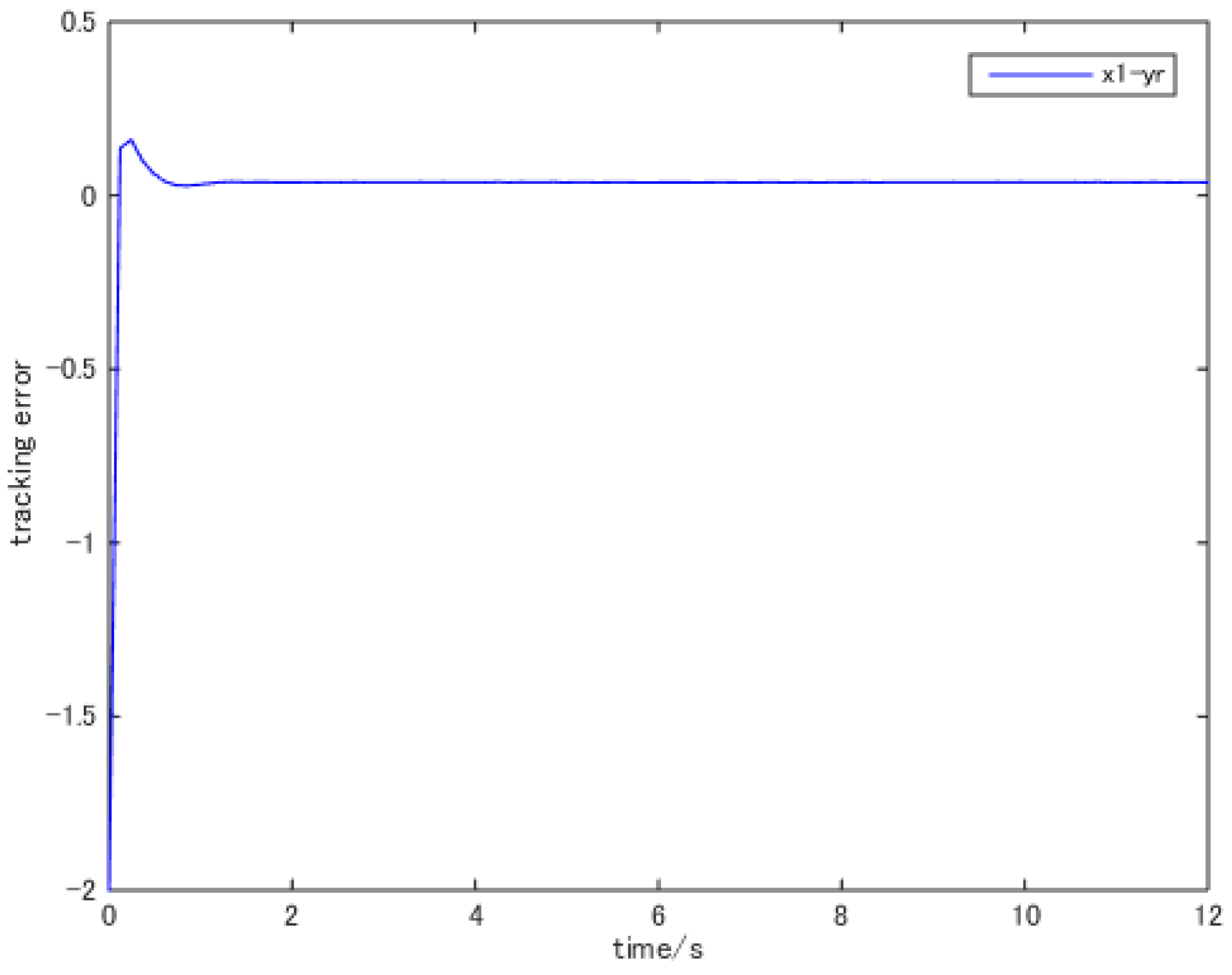
Figure 3.
The trajectory of state .
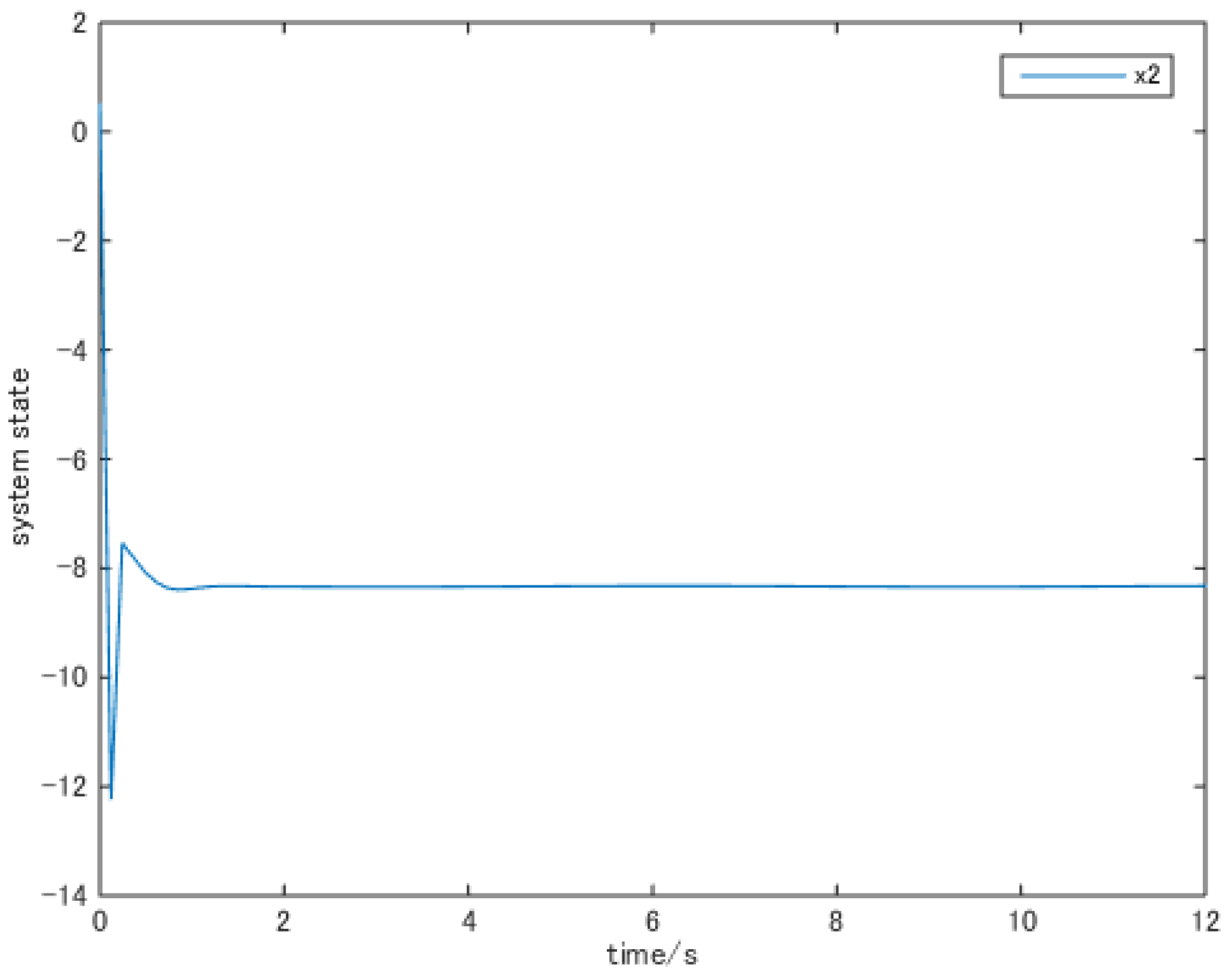
Figure 4.
The trajectory of state .

Publisher’s Note: MDPI stays neutral with regard to jurisdictional claims in published maps and institutional affiliations. |
© 2021 by the authors. Licensee MDPI, Basel, Switzerland. This article is an open access article distributed under the terms and conditions of the Creative Commons Attribution (CC BY) license (https://creativecommons.org/licenses/by/4.0/).
Share and Cite
MDPI and ACS Style
Alimhan, K.; Mamyrbayev, O.J.; Abdenova, G.A.; Akmetkalyeva, A. Output Tracking Control for High-Order Nonlinear Systems with Time Delay via Output Feedback Design. Symmetry 2021, 13, 675. https://doi.org/10.3390/sym13040675
AMA Style
Alimhan K, Mamyrbayev OJ, Abdenova GA, Akmetkalyeva A. Output Tracking Control for High-Order Nonlinear Systems with Time Delay via Output Feedback Design. Symmetry. 2021; 13(4):675. https://doi.org/10.3390/sym13040675
Chicago/Turabian StyleAlimhan, Keylan, Orken J. Mamyrbayev, Gaukhar A. Abdenova, and Almira Akmetkalyeva. 2021. "Output Tracking Control for High-Order Nonlinear Systems with Time Delay via Output Feedback Design" Symmetry 13, no. 4: 675. https://doi.org/10.3390/sym13040675
Note that from the first issue of 2016, this journal uses article numbers instead of page numbers. See further details here.