A New Quantile Regression for Modeling Bounded Data under a Unit Birnbaum–Saunders Distribution with Applications in Medicine and Politics

Abstract

Quantile regression provides a framework for modeling the relationship between a response variable and covariates using the quantile function. This work proposes a regression model for continuous variables bounded to the unit interval based on the unit Birnbaum–Saunders distribution as an alternative to the existing quantile regression models. By parameterizing the unit Birnbaum–Saunders distribution in terms of its quantile function allows us to model the effect of covariates across the entire response distribution, rather than only at the mean. Our proposal, especially useful for modeling quantiles using covariates, in general outperforms the other competing models available in the literature. These findings are supported by Monte Carlo simulations and applications using two real data sets. An R package, including parameter estimation, model checking as well as density, cumulative distribution, quantile and random number generating functions of the unit Birnbaum–Saunders distribution was developed and can be readily used to assess the suitability of our proposal.

1. Introduction

Recently, researchers are interested in deriving distributions with bounded support. Some of these distributions are the unit Birnbaum–Saunders (UBS) [1], unit gamma [2], unit Gompertz [3], unit inverse-Gaussian [4], unit Lindley [5,6], unit Weibull (UWEI) [7,8,9], and trapezoidal beta [10] models, among others.

This interest is due to several natural and anthropogenic phenomena are measured as indexes, percentages, proportions, rates and ratios, which are bounded on a certain interval, usually the unit interval. The need for modeling and analyzing bounded data occurs in many fields of real life such as in medicine [8], politics [11], and psychology [12]. Hence, to statistically describe this kind of data, distributions with bounded support are needed.

A series of distributions with support on the unit interval have been proposed in the literature based on transformations of the cumulative distribution function (CDF). Among them, we can mention the log-Bilai [13], log-shifted Gompertz [14], unit Gompertz [3], unit inverse-Gaussian [4], unit Lindley [5], and UWEI [8] distributions.

In order to assess the influence of one or more covariates on the mean of the distribution of a response variable bounded on the unit interval, the following distributions can be used: beta [15], beta rectangular [16], log-Bilai [13], log-Lindley [17], log-weighted exponential [18], quasi-beta [19], simplex [20], unit gamma [2], and unit Lindley [5,6,21]. To investigate the relationship between the response mode and covariates, we can consider the beta [22], Kumaraswamy (KUMA), unit gamma, and unit Gompertz [23] distributions.

The challenges in applied regression have been changing considerably, and full statistical modeling rather than predicting just means and modes is required in many applications [24]. Some parametric quantile regression models for bounded response that are available in the literature are based on the exponentiated arcsech-normal [25], Johnson-t [26], KUMA [27], log-extended exponential-geometric (LEEG) [28], L-logistic [29], power Johnson SB [30], unit Chen (UCHE) [31], unit half-normal (UHN) [32], unit Burr-XII (UBUR) [33], and UWEI [8] distributions. Unlike regression models through the mean, quantile regression, introduced in [34], allows one to model the effect of covariates across the entire response distribution. This motivates us to propose new quantile regression models.

Originated from problems of vibration in commercial aircraft that caused fatigue in the materials, Birnbaum and Saunders [35] introduced a skew positive distribution that has been extensively studied in the statistical literature. During the last decade, the Birnbaum–Saunders (BS) distribution has received significant attention by many researchers who generalized the BS distribution [36], studied its mathematical and statistical properties [37,38], estimated its parameters [39], and conducted regression modeling [40,41] and its diagnostic analysis [42]. BS quantile regression models and its diagnostics have been recently studied in [42,43,44,45].

As mentioned, an extension of the BS distribution for modeling bounded data was proposed in [1]. The authors showed that the UBS distribution is flexible and could be a good alternative to the beta and KUMA distributions for modeling data supported on the unit interval. In this context, considering the lack of agreement on preference and advantage of a specific model to describe bounded phenomena in a full statistical fashion, based on [42], we parameterize the UBS distribution using its quantile function (QF) to introduce a parametric quantile regression model. It is well-known that there are at least three approaches to modeling quantiles conditional on covariates, which are: (i) the distribution-free approach [34]; (ii) the approach based on a pseudo-likelihood through an asymmetric Laplace distribution [46]; and (iii) the parametric approach with the traditional maximum likelihood (ML) framework. The current manuscript is classified as the third category. To the best of our knowledge, quantile regression for modeling bounded data under a UBS distribution have not been proposed until now.

In this paper, we parameterize the UBS distribution in terms of its QF to evaluate the influence of one or more covariates on any quantile of the distribution of the response variable. This strategy was considered in [8,25,26,27,28,29,47] also to model responses on the standard unit interval. Other strategies were considered in [30,48,49]. For discrete and continuous positive responses, the literature is scarce and we can cite [42,50,51], who considered the discrete generalized half-normal distribution for discrete responses. Therefore, the objective of this investigation is to propose, derive and apply a UBS quantile regression model as an alternative to the existing quantile regression models.

The remainder of the paper is as follows. In Section 2, we introduce and characterize the UBS distribution in terms of its QF. The estimation method of parameters for the UBS distribution, based on the ML method, is discussed also here. The UBS quantile regression model is formulated in Section 3. A simulation study is carried out to evaluate the performance of the proposed results which are presented in Section 4. Applications considering two real data sets related to political sciences and sports medicine with seven competing models to the UBS quantile regression are analyzed in Section 5 and Section 6. Finally, Section 7 provides some conclusions and limitations of this work, as well as ideas for future investigation.

2. The Unit Birnbaum–Saunders Distribution

In this section, we parameterize the BS distribution in terms of its QF.

Considering the transformation $X=exp(-Y)$, where $Y\sim \mathrm{BS}(\alpha ,\beta )$, the UBS distribution was proposed in [1] with probability density function (PDF) and CDF written, respectively, as

$$f(x;\alpha ,\beta )=\frac{1}{2x\alpha \beta \sqrt{2\pi }}\left[{\left(-\frac{\beta }{log\left(x\right)}\right)}^{\frac{1}{2}}+{\left(-\frac{\beta }{log\left(x\right)}\right)}^{\frac{3}{2}}\right]exp\left[\frac{1}{2{\alpha }^2}\left(2+\frac{log\left(x\right)}{\beta }+\frac{\beta }{log\left(x\right)}\right)\right]$$

(1)

and

$$F(x;\alpha ,\beta )=1-\Phi \left\{\frac{1}{\alpha }\left[{\left(-\frac{log\left(x\right)}{\beta }\right)}^{\frac{1}{2}}-{\left(-\frac{\beta }{log\left(x\right)}\right)}^{\frac{1}{2}}\right]\right\},$$

(2)

where $0<x<1$, $\alpha >0$ is the shape parameter and $\Phi$ is the CDF of the standard normal distribution. It is noteworthy that $\delta =exp(-\beta )$ is a scale parameter and is also the median of the distribution of X, since $F(\delta ;\alpha ,\beta )=0.5$. In addition, the r-th moment of X is given by

$$\begin{array}{ccc}\hfill \mathrm{E}\left(X^r\right)& =& {\int }_0^1{x}^{r}f(x;\alpha ,\beta )\mathrm{d}x\hfill \\ & =& {\left.\begin{array}{c}f(x;\alpha ,\beta )\frac{x^{r+1}}{r+1}\end{array}\right|}_1^0-{\int }_0^1\frac{x^{r+1}}{r+1}{f}^{\prime }(x;\alpha ,\beta )\mathrm{d}x\hfill \\ & =& \frac{1}{2\left(2r{\alpha }^2\beta +1\right)}\left[2r{\alpha }^2\beta +{\left(2r{\alpha }^2\beta +1\right)}^{\frac{1}{2}}+1\right]exp\left[-\frac{{\left(2r{\alpha }^2\beta +1\right)}^{\frac{1}{2}}-1}{{\alpha }^2}\right],\hfill \end{array}$$

where $f^{\prime }\left(x;\alpha ,\beta \right)=\mathrm{d}f(x;\alpha ,\beta )/\mathrm{d}x$.

By inverting the CDF defined in (2), we have the QF stated as

$$Q\left(\tau ;\alpha ,\beta \right)=exp\left\{-\frac{2\beta }{2+{\left[\alpha {\Phi }^{-1}\left(1-\tau \right)\right]}^2-\alpha {\Phi }^{-1}\left(1-\tau \right)\sqrt{4+{\left[\alpha {\Phi }^{-1}\left(1-\tau \right)\right]}^2}}\right\},$$

(3)

where $0<\tau <1$ and ${\Phi }^{-1}$ is the QF of the standard normal distribution. Now, by solving the linear equation $Q(\tau ;\alpha ,\beta )-\mu =0$ in $\beta$ obtained from (3), we have

$$\beta =g^{-1}\left(\mu \right)=log\left(\mu \right)h\left(\alpha ,\tau \right),$$

(4)

where $h(\alpha ,\tau )=-\left(1/2\right)\{2+{\left[\alpha {\Phi }^{-1}(1-\tau )\right]}^2-\alpha {\Phi }^{-1}(1-\tau )\sqrt{4+\alpha {\Phi }^{-1}(1-\tau )}\},$ and $g^{-1}$ is the inverse function of g, which is assumed to be a quantile link function being strictly increasing, twice differentiable and mapping $(0,1)$ into $\mathbb{R}$.

Hence, we can parameterize (1) and (2), as a function of $\mu$, by means of

$$\begin{array}{ccc}\hfill f(x;\mu ,\alpha ,\tau )& =& \frac{1}{2x\alpha log\left(\mu \right)h\left(\alpha ,\tau \right)\sqrt{2\pi }}\left\{{\left[-\frac{log\left(\mu \right)h\left(\alpha ,\tau \right)}{log\left(x\right)}\right]}^{\frac{1}{2}}+{\left[-\frac{log\left(\mu \right)h\left(\alpha ,\tau \right)}{log\left(x\right)}\right]}^{\frac{3}{2}}\right\}\hfill \\ & & \hfill \\ & & \times exp\left\{\frac{1}{2{\alpha }^2}\left[\frac{log\left(x\right)}{log\left(\mu \right)h\left(\alpha ,\tau \right)}+\frac{log\left(\mu \right)h\left(\alpha ,\tau \right)}{log\left(x\right)}+2\right]\right\}\hfill \end{array}$$

(5)

and

$$F(x;\mu ,\alpha ,\tau )=1-\Phi \left\{\frac{1}{\alpha }\left[{\left(-\frac{log\left(x\right)}{log\left(\mu \right)h\left(\alpha ,\tau \right)}\right)}^{\frac{1}{2}}-{\left(-\frac{log\left(\mu \right)h\left(\alpha ,\tau \right)}{log\left(x\right)}\right)}^{\frac{1}{2}}\right]\right\},$$

(6)

where $0<x<1$, $0<\mu <1$, $\alpha >0$, and $\tau$ is fixed.

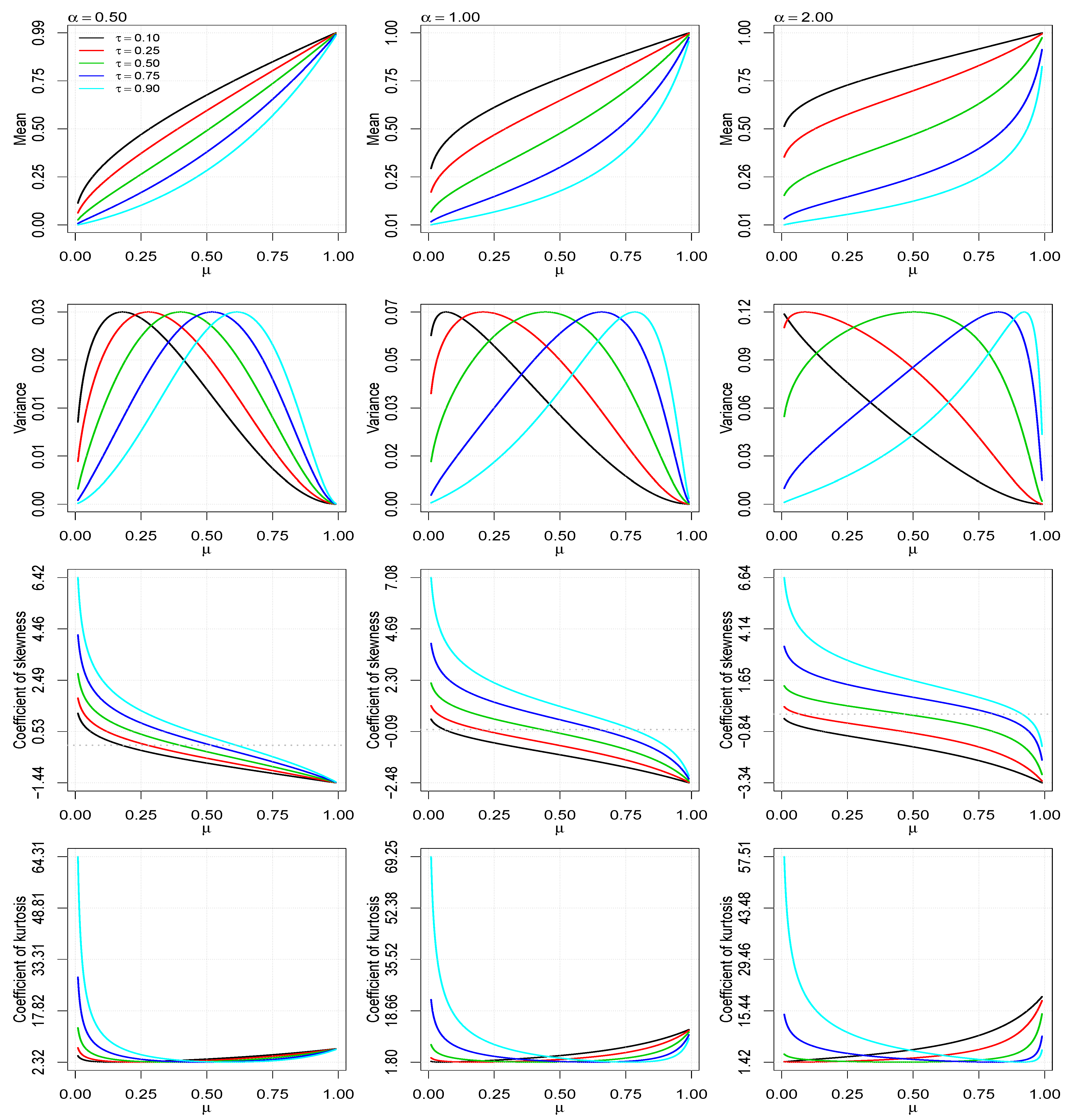
Figure 1 shows some possible shapes of the PDF of the UBS distribution for selected values of the parameters $\mu$, $\alpha$ and $\tau$. The behaviors of the mean, variance, coefficient of skewness and coefficient of kurtosis are shown in Figure 2.

An advantage of the parameterization stated in (5) and (6) is that $\mu$ is the $\tau$-th quantile and, consequently, the interpretation of this parameterization becomes more interesting in applications. Furthermore, it is possible to consider that the parameter $\mu$ depends on covariates; see Section 3.

The standard ML method can be used to estimate the UBS parameters by maximizing the corresponding log-likelihood function. Let $\mathit{x}=\left(x_1,\dots ,x_n\right)$ be a realization of the random sample $\mathit{X}=\left(X_1,\dots ,X_n\right)$, where $X_1,\dots ,X_n$ are independent and identically distributed random variables according to (1). Using (5), the corresponding log-likelihood function, with $\mathit{\theta }=(\mu ,\alpha )$, is written as

$$\begin{array}{ccc}\hfill \ell \left(\mathit{\theta };\mathit{x},\tau \right)& \propto & -nlog\left[\alpha log\left(\mu \right)h\left(\alpha ,\tau \right)\right]+\frac{n}{{\alpha }^2}+\frac{1}{2{\alpha }^2}\sum _{i=1}^n\frac{log\left(x_i\right)}{log\left(\mu \right)h\left(\alpha ,\tau \right)}\hfill \\ & & +\sum _{i=1}^{n}log\left\{{\left[-\frac{log\left(\mu \right)h\left(\alpha ,\tau \right)}{log\left(x_i\right)}\right]}^{\frac{1}{2}}+{\left[-\frac{log\left(\mu \right)h\left(\alpha ,\tau \right)}{log\left(x_i\right)}\right]}^{\frac{3}{2}}\right\}+\frac{1}{2{\alpha }^2}\sum _{i=1}^n\frac{log\left(\mu \right)h\left(\alpha ,\tau \right)}{log\left(x_i\right)}.\hfill \end{array}$$

Defining $\mathit{U}\left(\mathit{\theta };\mathit{x},\tau \right)=\left(U_{\mu },U_{\alpha }\right)$, where $U_{\mu }=\partial \ell \left(\mathit{\theta };\mathit{x},\tau \right)/\partial \mu$, $U_{\alpha }=\partial \ell \left(\mathit{\theta };\mathit{x},\tau \right)/\partial \alpha$, and $h^{\prime }\left(\alpha ,\tau \right)=\partial h\left(\alpha ,\tau \right)/\partial \alpha$, we get the associated score vector with coordinates stated as

$$\begin{array}{ccc}\hfill U_{\mu }& =& -\frac{n}{\mu log\left(\mu \right)}-\frac{1}{2{\alpha }^2}\sum _{i=1}^n\frac{log\left(x_i\right)}{log{\left(\mu \right)}^{2}h\left(\alpha ,\tau \right)}+\frac{1}{2{\alpha }^2}\sum _{i=1}^n\frac{h\left(\alpha ,\tau \right)}{\mu log\left(x_i\right)}\hfill \\ \hfill \\ \hfill & & -\frac{1}{2}\sum _{i=1}^n\frac{log\left(x_i\right)-3log\left(\mu \right)h\left(\alpha ,\tau \right)}{log\left(\mu \right)\mu \left[log\left(\mu \right)h\left(\alpha ,\tau \right)-log\left(x_i\right)\right]},\hfill \end{array}$$

(7)

$$\begin{array}{ccc}\hfill U_{\alpha }& =& -\frac{2n}{{\alpha }^3}-\frac{n}{\alpha h\left(\alpha ,\tau \right)}\left[h\left(\alpha ,\tau \right)+\alpha h^{\prime }\left(\alpha ,\tau \right)\right]-\frac{\left[2h\left(\alpha ,\tau \right)+h^{\prime }\left(\alpha ,\tau \right)\alpha \right]}{2{\alpha }^{3}log\left(\mu \right)h{\left(\alpha ,\tau \right)}^2}\sum _{i=1}^{n}log\left(x_i\right)\hfill \\ \hfill \\ \hfill & & +\frac{h^{\prime }\left(\alpha ,\tau \right)}{2h\left(\alpha ,\tau \right)}\sum _{i=1}^n\frac{log\left(x_i\right)-3log\left(\mu \right)h\left(\alpha ,\tau \right)}{log\left(x_i\right)-log\left(\mu \right)h\left(\alpha ,\tau \right)}-\frac{log\left(\mu \right)\left[2h\left(\alpha ,\tau \right)-h^{\prime }\left(\alpha ,\tau \right)\alpha \right]}{2{\alpha }^3}\sum _{i=1}^n\frac{1}{log\left(x_i\right)}.\hfill \end{array}$$

(8)

By solving numerically the system of non-linear equations in $\mu$ and $\alpha$, formed by the coordinates of $\mathit{U}\left(\mathit{\theta };\mathit{x},\tau \right)$ defined in (7) and (8), we have the ML estimate of $\widehat{\mathit{\theta }}$. The asymptotic standard errors (SEs) of the corresponding estimators are obtained by inverting the Hessian matrix of the log-likelihood function. This Hessian matrix is generated by taking the second derivative of (7), with respect to $\mu$ and $\alpha$.

For $\tau =0.5$, we have that

$$\widehat{\alpha }=\frac{1}{nlog\left(\widehat{\mu }\right)}\sqrt{nlog\left(\widehat{\mu }\right)\left[\sum _{i=1}^{n}log\left(x_i\right)+{log}^2\left(\widehat{\mu }\right)\sum _{i=1}^n\frac{1}{log\left(x_i\right)}-2nlog\left(\widehat{\mu }\right)\right]}=\xi \left(\widehat{\mu }\right),$$

while $\widehat{\mu }$ must be found numerically taking $\alpha =\xi \left(\widehat{\mu }\right)$ in the expression defined in (7).

3. The UBS Quantile Regression Model

In this section, considering the parameterized PDF stated in (5), we formulate the UBS quantile regression model.

Let $X_1,\dots ,X_n$ be n independent random variables, where each $X_i$, for $i=1,\dots ,n$, follows the PDF given in (5) with unknown quantile parameter ${\mu }_i$, unknown shape parameter $\alpha$, and $\tau \in (0,1)$ is assumed as fixed, that is, $X_i\sim \mathrm{UBS}({\mu }_i,\alpha ;\tau )$. Here, the UBS quantile regression model is defined imposing that the quantile ${\mu }_i$ of $X_i$ satisfies the functional relation expressed by

$$g\left({\mu }_i\right)={\mathit{z}}_i^{\top }\mathit{\delta },i=1,\dots ,n,$$

(9)

where $\mathit{\delta }={({\delta }_0,\dots ,{\delta }_{p-1})}^{\top }$ is a p-dimensional vector of unknown regression coefficients, with $p<n$ and n being the sample size, ${\mathit{z}}_i={(1,z_{i1},\dots ,z_{i(p-1)})}^{\top }$ denotes the observations on p known covariates, and g is given as in (4). There are several possibilities for the link function g stated in (9). For instance, the most useful well-known link functions are:

(i)

[Logit] $g\left({\mu }_i\right)=log\left[{\mu }_i/(1-{\mu }_i)\right]$;

(ii)

[Probit] $g\left({\mu }_i\right)={\Phi }^{-1}\left({\mu }_i\right)$;

(iii)

[Complementary log-log] $g\left({\mu }_i\right)=log\left[-log(1-{\mu }_i)\right]$;

(iv)

[Log-log] $g\left({\mu }_i\right)=log[-log\left({\mu }_i\right)]$; and

(v)

[Cauchit] $g\left({\mu }_i\right)=tan\left[\pi (\mu -0.5)\right]$;

which are the inverse CDF of the logistic, standard normal, minimum extreme-value, maximum extreme-value and Cauchy distributions, respectively.

Let $X_1,\dots ,X_n$ be n independent random variables such that $X_i\sim \mathrm{UBS}({\mu }_i,\alpha ;\tau )$ denotes a UBS distributed random variable and consider that

$${\mu }_i={\displaystyle \frac{exp\left({\mathit{z}}_i^{\top }\mathit{\delta }\right)}{1+exp\left({\mathit{z}}_i^{\top }\mathit{\delta }\right)}},i=1,\dots ,n,$$

to ensure that the predicted quantiles lie within the unit interval.

For fixed $\tau \in (0,1),$ let now $\mathit{\theta }={({\mathit{\delta }}^{\top },\alpha )}^{\top }$ be the vector of $p+1$ unknown parameters to be estimated. The ML estimate $\widehat{\mathit{\theta }}={({\widehat{\mathit{\delta }}}^{\top },\widehat{\alpha })}^{\top }$ of $\mathit{\theta }$ is obtained by the maximizing the log-likelihood function stated in (7). It is not possible to derive analytical solution for the ML estimate $\widehat{\mathit{\theta }}$ so that it must be calculated numerically using some optimization algorithm such as Newton-Raphson and quasi-Newton. Based on [15], we suggest to use, as an initial guess for $\mathit{\delta }$, the ordinary least squares estimate of this parameter vector obtained from the linear regression of the transformed responses $g\left(x_1\right),\dots ,g\left(x_n\right)$ on $\mathit{Z}$, that is, $\widehat{\mathit{\delta }}={\left({\mathit{Z}}^{\top }\mathit{Z}\right)}^{-1}{Z}^{\top }\mathit{w}$, where $\mathit{w}={(g\left(x_1\right),\dots ,g\left(x_n\right))}^{\top }$.

Under mild regularity conditions and when the sample size n is large, the asymptotic distribution of the ML estimator $\widehat{\mathit{\theta }}={({\widehat{\mathit{\delta }}}^{\top },\widehat{\alpha })}^{\top }$ is approximately multivariate normal (of dimension $p+1$) with mean vector $\mathit{\theta }={({\mathit{\delta }}^{\top },\alpha )}^{\top }$ and variance covariance matrix ${\mathit{K}}^{-1}\left(\mathit{\theta }\right)$, where

$$\mathit{K}\left(\mathit{\theta }\right)=\mathrm{E}\left[-\frac{\partial \ell \left(\mathit{\theta }\right)}{\partial \mathit{\theta }\partial {\mathit{\theta }}^{\top }}\right]$$

is the expected Fisher information matrix. Note that there is no closed form expression for the matrix $\mathit{K}\left(\mathit{\theta }\right)$. Nevertheless, as shown in [52], the estimated observed Fisher information matrix

$$\mathit{J}\left(\widehat{\mathit{\theta }}\right)=-\frac{\partial \ell \left(\mathit{\theta }\right)}{\partial \mathit{\theta }\partial {\mathit{\theta }}^{\top }}{|}_{\mathit{\theta }=\widehat{\mathit{\theta }}}$$

is a consistent estimator of the expected Fisher information matrix $\mathit{K}\left(\mathit{\theta }\right)$. Therefore, for large n, we can replace $\mathit{K}\left(\mathit{\theta }\right)$ by $\mathit{J}\left(\widehat{\mathit{\theta }}\right)$.

Let ${\theta }_r$ be the r-th component of $\mathit{\theta }$. The asymptotic $100\times (1-\gamma )\%$ confidence interval for ${\theta }_r$ is given by $[{\widehat{\theta }}_r\pm z_{\gamma /2}\widehat{\mathrm{SE}}\left({\widehat{\theta }}_r\right)]$, with $r=1,\dots ,p+1$, where $z_{\gamma /2}$ is the $100\times \gamma /2$ upper quantile of the standard normal distribution and $\widehat{\mathrm{SE}}\left({\widehat{\theta }}_r\right)$ is the estimated asymptotic SE of ${\widehat{\theta }}_r$. Note that $\widehat{\mathrm{SE}}\left({\widehat{\theta }}_r\right)$ is the square root of the r-th diagonal element of the matrix ${\mathit{J}}^{-1}\left(\widehat{\mathit{\theta }}\right)$.

Given n pairs of observations $(x_i,{\mathit{z}}_i)$, the parameter estimates of $\mathit{\delta }={({\delta }_0,\dots ,{\delta }_{p-1})}^{\top }$ and $\alpha$ can be obtained directly through a library of the R software named unitBSQuantReg by means of its function unitBSQuantReg(formula, tau, data, link,…). For model checking, the function hnp(object, nsim = 99, halfnormal = TRUE, plot = TRUE, level = 0.95,

resid.type = c(“cox-snell”, “quantile”)) is available, which provides half-normal probability plots with simulated envelopes. A version of the unitBSQuantReg package is available at https://github.com/AndrMenezes/unitBSQuantReg (accessed on 9 April 2021).

Due to the direct interpretation of the parameters in terms of odds, in this paper, we consider only the logit link. When ${\mu }_i$ is the $\tau$-th quantile, for $0<\tau <1$, the interpretations are straightforward. In addition, a strictly positive link function relating the shape parameter $\beta$ with covariates ${\mathit{w}}_i$, not necessarily equal to ${\mathit{x}}_i$, can be considered. Of course, other link functions might be explored.

4. A Monte Carlo Simulation Study

In this section, we present the results of the Monte Carlo simulations used to assess the empirical bias and root mean-squared error (RMSE) of the ML estimators of the UBS quantile regression parameters. We also present the coverage probability (CP) of the $95\%$ confidence interval (CP${}_{95\%}$) based on asymptotic normality of the ML estimators. We consider sample sizes $n=20,50,100,200,300$; $\tau =0.10,0.25,0.50,0.75,0.90$; $\alpha =0.5,1.0,2.0$, and two regression frameworks formulated as

(i)

$\mathrm{logit}\left({\mu }_i\right)={\delta }_0+{\delta }_1{z}_{i1}$ for ${\delta }_0=1.0$, ${\delta }_1=2.0$, with $z_{i1}\sim \mathrm{N}(0,1)$; and

(ii)

$\mathrm{logit}\left({\mu }_i\right)={\delta }_0+{\delta }_1{z}_{i1}+{\delta }_2{z}_{i2}$ for ${\delta }_0=1.0$, ${\delta }_1=1.0$, ${\delta }_2=2.0$, $z_{i1}\sim \mathrm{N}(0,1)$, with $z_{i2}\sim \mathrm{N}(0,1)$.

For each combination of $(n,\tau ,\alpha )$ and both regression frameworks (the covariate(s) remained constant throughout the simulations), $B=5000$ pseudo-random samples were simulated using the SAS Data-Step, while parameter estimates were obtained by the quasi-Newton method in SAS PROC NLMIXED. The values of the response variable, given n, $\tau$, $\alpha$ and the covariate(s), are generated from the quantile function stated as

$$q=exp\left(-2\beta /\left\{2+{\left[\alpha {\Phi }^{-1}\left(1-U\right)\right]}^2-\alpha {\Phi }^{-1}\left(1-U\right)\sqrt{4+{\left[\alpha {\Phi }^{-1}\left(1-U\right)\right]}^2}\right\}\right),$$

where $U\sim \mathrm{U}(0,1)$ and $\beta =log\left(\mu \right)h(\alpha ,\tau )$ for $h(\alpha ,\tau )$ defined in (4).

The empirical bias, RMSE and CP are calculated, respectively, by

(i)

Bias$\left(\widehat{\varrho }\right)=(1/B){\sum }_{i=1}^B({\widehat{\varrho }}_i-\varrho )$;

(ii)

RMSE$\left({\widehat{\varrho }}_i\right)={\left[(1/B){\sum }_{i=1}^B{({\widehat{\varrho }}_i-\varrho )}^2\right]}^{1/2}$; and

(iii)

CP${}_{95\%}\left({\widehat{\varrho }}_i\right)=(1/B){\sum }_{i=1}^{B}I[{\widehat{\varrho }}_i\pm 1.96\mathrm{SE}\left({\widehat{\varrho }}_i\right)]$, where $\varrho =\alpha ,{\delta }_0,{\delta }_1$, or ${\delta }_2$, I is the indicator function, and $\mathrm{SE}\left({\widehat{\varrho }}_i\right)$ is the corresponding estimated SE.

Table 1. Empirical bias, RMSE and $95\%$ CP for the true values ${\delta }_0=1.0$, ${\delta }_1=2.0$ and $\alpha =0.5$ of the indicated quantile level ($\tau$), sample size (n) and parameter (${\delta }_0,{\delta }_1,\alpha$) with simulated data.

$\mathit{\tau }$	n	Bias			RMSE			CP${}_{95\%}$
		${\mathit{\delta }}_{\mathbf{0}}$	${\mathit{\delta }}_{\mathbf{1}}$	$\mathit{\alpha }$	${\mathit{\delta }}_{\mathbf{0}}$	${\mathit{\delta }}_{\mathbf{1}}$	$\mathit{\alpha }$	${\mathit{\delta }}_{\mathbf{0}}$	${\mathit{\delta }}_{\mathbf{1}}$	$\mathit{\alpha }$
0.10	20	$0.050$	$-0.007$	$-0.034$	$0.202$	$0.174$	$0.085$	$0.887$	$0.916$	$0.853$
	50	$0.021$	$-0.003$	$-0.013$	$0.123$	$0.103$	$0.051$	$0.927$	$0.938$	$0.911$
	100	$0.010$	$-0.002$	$-0.006$	$0.087$	$0.073$	$0.036$	$0.936$	$0.940$	$0.932$
	200	$0.005$	$-0.001$	$-0.003$	$0.061$	$0.051$	$0.025$	$0.943$	$0.944$	$0.941$
	300	$0.003$	$-0.000$	$-0.002$	$0.050$	$0.041$	$0.020$	$0.948$	$0.947$	$0.946$
0.25	20	$0.026$	$-0.002$	$-0.034$	$0.168$	$0.173$	$0.086$	$0.903$	$0.918$	$0.854$
	50	$0.011$	$-0.002$	$-0.013$	$0.103$	$0.102$	$0.051$	$0.935$	$0.940$	$0.911$
	100	$0.005$	$-0.001$	$-0.006$	$0.073$	$0.072$	$0.036$	$0.940$	$0.941$	$0.931$
	200	$0.003$	$-0.000$	$-0.003$	$0.051$	$0.050$	$0.025$	$0.944$	$0.945$	$0.940$
	300	$0.002$	$-0.000$	$-0.002$	$0.042$	$0.041$	$0.020$	$0.950$	$0.947$	$0.946$
0.50	20	$-0.003$	$0.004$	$-0.034$	$0.152$	$0.172$	$0.086$	$0.918$	$0.918$	$0.856$
	50	$-0.000$	$0.001$	$-0.013$	$0.094$	$0.102$	$0.051$	$0.938$	$0.941$	$0.912$
	100	$-0.000$	$-0.000$	$-0.006$	$0.066$	$0.072$	$0.036$	$0.944$	$0.943$	$0.932$
	200	$0.000$	$0.000$	$-0.003$	$0.047$	$0.050$	$0.025$	$0.946$	$0.946$	$0.940$
	300	$0.000$	$0.000$	$-0.002$	$0.038$	$0.040$	$0.020$	$0.949$	$0.949$	$0.947$
0.75	20	$-0.033$	$0.011$	$-0.034$	$0.171$	$0.174$	$0.085$	$0.914$	$0.920$	$0.855$
	50	$-0.012$	$0.003$	$-0.013$	$0.104$	$0.103$	$0.051$	$0.934$	$0.944$	$0.914$
	100	$-0.006$	$0.001$	$-0.006$	$0.073$	$0.072$	$0.036$	$0.944$	$0.942$	$0.933$
	200	$-0.003$	$0.001$	$-0.003$	$0.052$	$0.050$	$0.025$	$0.946$	$0.946$	$0.940$
	300	$-0.002$	$0.001$	$-0.002$	$0.042$	$0.041$	$0.020$	$0.948$	$0.949$	$0.947$
0.90	20	$-0.058$	$0.018$	$-0.033$	$0.207$	$0.177$	$0.085$	$0.904$	$0.920$	$0.857$
	50	$-0.022$	$0.006$	$-0.013$	$0.125$	$0.104$	$0.051$	$0.930$	$0.944$	$0.915$
	100	$-0.011$	$0.002$	$-0.006$	$0.087$	$0.073$	$0.036$	$0.941$	$0.942$	$0.935$
	200	$-0.005$	$0.002$	$-0.003$	$0.061$	$0.051$	$0.025$	$0.947$	$0.947$	$0.939$
	300	$-0.003$	$0.001$	$-0.002$	$0.049$	$0.041$	$0.020$	$0.950$	$0.949$	$0.945$

,

Table 2. Empirical bias, RMSE and $95\%$ CP for the true values ${\delta }_0=1.0$, ${\delta }_1=2.0$ and $\alpha =1.0$ of the indicated quantile level ($\tau$), sample size (n) and parameter (${\delta }_0,{\delta }_1,\alpha$) with simulated data.

$\mathit{\tau }$	n	Bias			RMSE			CP${}_{95\%}$
		${\mathit{\delta }}_{\mathbf{0}}$	${\mathit{\delta }}_{\mathbf{1}}$	$\mathit{\alpha }$	${\mathit{\delta }}_{\mathbf{0}}$	${\mathit{\delta }}_{\mathbf{1}}$	$\mathit{\alpha }$	${\mathit{\delta }}_{\mathbf{0}}$	${\mathit{\delta }}_{\mathbf{1}}$	$\mathit{\alpha }$
0.10	20	$0.094$	$-0.007$	$-0.073$	$0.367$	$0.320$	$0.173$	$0.884$	$0.918$	$0.846$
	50	$0.038$	$-0.005$	$-0.029$	$0.222$	$0.189$	$0.103$	$0.925$	$0.939$	$0.908$
	100	$0.018$	$-0.003$	$-0.014$	$0.157$	$0.133$	$0.072$	$0.936$	$0.941$	$0.930$
	200	$0.009$	$-0.001$	$-0.007$	$0.110$	$0.092$	$0.050$	$0.944$	$0.946$	$0.939$
	300	$0.006$	$-0.000$	$-0.004$	$0.089$	$0.075$	$0.041$	$0.948$	$0.947$	$0.945$
0.25	20	$0.050$	$0.001$	$-0.073$	$0.312$	$0.318$	$0.173$	$0.901$	$0.918$	$0.847$
	50	$0.021$	$-0.002$	$-0.029$	$0.190$	$0.188$	$0.103$	$0.934$	$0.940$	$0.908$
	100	$0.010$	$-0.002$	$-0.014$	$0.134$	$0.131$	$0.072$	$0.938$	$0.942$	$0.930$
	200	$0.005$	$0.000$	$-0.007$	$0.095$	$0.092$	$0.050$	$0.944$	$0.946$	$0.939$
	300	$0.003$	$0.000$	$-0.004$	$0.077$	$0.074$	$0.041$	$0.949$	$0.948$	$0.945$
0.50	20	$-0.010$	$0.013$	$-0.073$	$0.283$	$0.320$	$0.173$	$0.916$	$0.922$	$0.847$
	50	$-0.003$	$0.003$	$-0.029$	$0.172$	$0.188$	$0.103$	$0.939$	$0.942$	$0.909$
	100	$-0.001$	$0.000$	$-0.014$	$0.121$	$0.131$	$0.072$	$0.945$	$0.944$	$0.930$
	200	$-0.000$	$0.001$	$-0.007$	$0.085$	$0.091$	$0.050$	$0.945$	$0.946$	$0.940$
	300	$-0.000$	$0.001$	$-0.004$	$0.069$	$0.074$	$0.041$	$0.948$	$0.948$	$0.946$
0.75	20	$-0.074$	$0.029$	$-0.072$	$0.325$	$0.327$	$0.173$	$0.915$	$0.923$	$0.849$
	50	$-0.028$	$0.009$	$-0.029$	$0.194$	$0.190$	$0.103$	$0.936$	$0.944$	$0.910$
	100	$-0.013$	$0.003$	$-0.014$	$0.135$	$0.132$	$0.072$	$0.945$	$0.944$	$0.931$
	200	$-0.006$	$0.002$	$-0.007$	$0.095$	$0.092$	$0.050$	$0.946$	$0.947$	$0.939$
	300	$-0.004$	$0.002$	$-0.004$	$0.077$	$0.074$	$0.041$	$0.950$	$0.948$	$0.946$
0.90	20	$-0.122$	$0.043$	$-0.071$	$0.390$	$0.335$	$0.171$	$0.908$	$0.924$	$0.850$
	50	$-0.047$	$0.014$	$-0.028$	$0.228$	$0.192$	$0.102$	$0.932$	$0.946$	$0.912$
	100	$-0.023$	$0.005$	$-0.014$	$0.158$	$0.133$	$0.071$	$0.943$	$0.944$	$0.933$
	200	$-0.010$	$0.003$	$-0.007$	$0.111$	$0.093$	$0.050$	$0.947$	$0.947$	$0.939$
	300	$-0.007$	$0.002$	$-0.004$	$0.089$	$0.075$	$0.040$	$0.949$	$0.950$	$0.945$

and

Table 3. Empirical bias, RMSE and $95\%$ CP for the true values ${\delta }_0=1.0$, ${\delta }_1=2.0$ and $\alpha =2.0$ of the indicated quantile level ($\tau$), sample size (n) and parameter (${\delta }_0,{\delta }_1,\alpha$) with simulated data.

$\mathit{\tau }$	n	Bias			RMSE			CP${}_{95\%}$
		${\mathit{\delta }}_{\mathbf{0}}$	${\mathit{\delta }}_{\mathbf{1}}$	$\mathit{\alpha }$	${\mathit{\delta }}_{\mathbf{0}}$	${\mathit{\delta }}_{\mathbf{1}}$	$\mathit{\alpha }$	${\mathit{\delta }}_{\mathbf{0}}$	${\mathit{\delta }}_{\mathbf{1}}$	$\mathit{\alpha }$
0.10	20	$0.152$	$-0.004$	$-0.162$	$0.566$	$0.511$	$0.358$	$0.887$	$0.921$	$0.831$
	50	$0.061$	$-0.005$	$-0.064$	$0.333$	$0.292$	$0.209$	$0.928$	$0.941$	$0.901$
	100	$0.029$	$-0.004$	$-0.031$	$0.233$	$0.201$	$0.145$	$0.938$	$0.941$	$0.928$
	200	$0.014$	$-0.001$	$-0.015$	$0.163$	$0.139$	$0.101$	$0.945$	$0.947$	$0.938$
	300	$0.009$	$0.000$	$-0.009$	$0.132$	$0.112$	$0.081$	$0.950$	$0.947$	$0.944$
0.25	20	$0.095$	$0.006$	$-0.162$	$0.502$	$0.512$	$0.358$	$0.897$	$0.922$	$0.833$
	50	$0.039$	$-0.002$	$-0.064$	$0.297$	$0.291$	$0.210$	$0.930$	$0.942$	$0.901$
	100	$0.019$	$-0.002$	$-0.031$	$0.208$	$0.200$	$0.145$	$0.941$	$0.943$	$0.928$
	200	$0.010$	$0.000$	$-0.015$	$0.146$	$0.138$	$0.101$	$0.946$	$0.947$	$0.938$
	300	$0.006$	$0.001$	$-0.009$	$0.118$	$0.111$	$0.082$	$0.948$	$0.946$	$0.944$
0.50	20	$-0.026$	$0.032$	$-0.160$	$0.450$	$0.522$	$0.358$	$0.917$	$0.924$	$0.832$
	50	$-0.008$	$0.007$	$-0.063$	$0.262$	$0.292$	$0.210$	$0.939$	$0.943$	$0.903$
	100	$-0.004$	$0.002$	$-0.030$	$0.181$	$0.199$	$0.145$	$0.945$	$0.944$	$0.929$
	200	$-0.001$	$0.002$	$-0.014$	$0.127$	$0.138$	$0.101$	$0.946$	$0.946$	$0.938$
	300	$-0.001$	$0.002$	$-0.009$	$0.102$	$0.111$	$0.082$	$0.949$	$0.948$	$0.945$
0.75	20	$-0.157$	$0.069$	$-0.158$	$0.558$	$0.549$	$0.356$	$0.922$	$0.928$	$0.833$
	50	$-0.058$	$0.020$	$-0.062$	$0.311$	$0.299$	$0.208$	$0.941$	$0.945$	$0.905$
	100	$-0.028$	$0.008$	$-0.030$	$0.212$	$0.202$	$0.144$	$0.947$	$0.945$	$0.929$
	200	$-0.013$	$0.005$	$-0.014$	$0.148$	$0.139$	$0.101$	$0.946$	$0.946$	$0.938$
	300	$-0.009$	$0.004$	$-0.009$	$0.119$	$0.111$	$0.081$	$0.949$	$0.949$	$0.946$
0.90	20	$-0.227$	$0.087$	$-0.160$	$0.653$	$0.569$	$0.354$	$0.918$	$0.930$	$0.833$
	50	$-0.083$	$0.024$	$-0.065$	$0.353$	$0.303$	$0.208$	$0.938$	$0.947$	$0.904$
	100	$-0.040$	$0.007$	$-0.033$	$0.238$	$0.203$	$0.144$	$0.945$	$0.946$	$0.928$
	200	$-0.020$	$0.003$	$-0.018$	$0.166$	$0.140$	$0.101$	$0.947$	$0.946$	$0.935$
	300	$-0.014$	$0.001$	$-0.013$	$0.133$	$0.112$	$0.081$	$0.948$	$0.950$	$0.942$

and

Table 4. Empirical bias, RMSE and $95\%$ CP for the true values ${\delta }_0=1.0$, ${\delta }_1=1.0$, ${\delta }_2=2.0$ and $\alpha =0.5$ of the indicated quantile level ($\tau$), sample size (n) and parameter (${\delta }_0,{\delta }_1,\alpha$) with simulated data.

$\mathit{\tau }$	n	Bias				RMSE				CP${}_{95\%}$
		${\mathit{\delta }}_{\mathbf{0}}$	${\mathit{\delta }}_{\mathbf{1}}$	${\mathit{\delta }}_{\mathbf{2}}$	$\mathit{\alpha }$	${\mathit{\delta }}_{\mathbf{0}}$	${\mathit{\delta }}_{\mathbf{1}}$	${\mathit{\delta }}_{\mathbf{2}}$	$\mathit{\alpha }$	${\mathit{\delta }}_{\mathbf{0}}$	${\mathit{\delta }}_{\mathbf{1}}$	${\mathit{\delta }}_{\mathbf{2}}$	$\mathit{\alpha }$
0.10	20	$0.066$	$-0.006$	$-0.010$	$-0.046$	$0.213$	$0.160$	$0.176$	$0.091$	$0.876$	$0.916$	$0.912$	$0.813$
	50	$0.027$	$-0.002$	$-0.005$	$-0.019$	$0.128$	$0.095$	$0.103$	$0.052$	$0.920$	$0.930$	$0.938$	$0.901$
	100	$0.013$	$-0.001$	$-0.002$	$-0.009$	$0.090$	$0.065$	$0.073$	$0.036$	$0.933$	$0.939$	$0.941$	$0.924$
	200	$0.006$	$-0.000$	$-0.001$	$-0.005$	$0.063$	$0.045$	$0.051$	$0.025$	$0.939$	$0.946$	$0.945$	$0.934$
	300	$0.004$	$-0.001$	$-0.000$	$-0.003$	$0.052$	$0.036$	$0.041$	$0.021$	$0.941$	$0.948$	$0.945$	$0.940$
0.25	20	$0.033$	$-0.003$	$-0.003$	$-0.047$	$0.176$	$0.160$	$0.175$	$0.091$	$0.898$	$0.916$	$0.915$	$0.812$
	50	$0.014$	$-0.001$	$-0.002$	$-0.019$	$0.107$	$0.095$	$0.102$	$0.053$	$0.928$	$0.930$	$0.940$	$0.899$
	100	$0.007$	$-0.000$	$-0.001$	$-0.009$	$0.075$	$0.065$	$0.072$	$0.037$	$0.940$	$0.939$	$0.942$	$0.924$
	200	$0.003$	$-0.000$	$-0.000$	$-0.005$	$0.053$	$0.045$	$0.050$	$0.026$	$0.941$	$0.946$	$0.946$	$0.934$
	300	$0.002$	$-0.000$	$0.000$	$-0.003$	$0.043$	$0.036$	$0.041$	$0.021$	$0.941$	$0.947$	$0.944$	$0.939$
0.50	20	$-0.008$	$0.001$	$0.005$	$-0.047$	$0.158$	$0.161$	$0.175$	$0.092$	$0.914$	$0.917$	$0.919$	$0.813$
	50	$-0.003$	$0.001$	$0.001$	$-0.019$	$0.097$	$0.095$	$0.102$	$0.053$	$0.937$	$0.930$	$0.941$	$0.895$
	100	$-0.001$	$0.000$	$0.001$	$-0.009$	$0.069$	$0.065$	$0.072$	$0.037$	$0.940$	$0.938$	$0.943$	$0.922$
	200	$-0.001$	$0.000$	$0.001$	$-0.005$	$0.048$	$0.045$	$0.050$	$0.026$	$0.945$	$0.947$	$0.947$	$0.931$
	300	$-0.001$	$-0.000$	$0.001$	$-0.003$	$0.039$	$0.036$	$0.041$	$0.021$	$0.944$	$0.947$	$0.944$	$0.939$
0.75	20	$-0.049$	$0.006$	$0.015$	$-0.046$	$0.180$	$0.162$	$0.177$	$0.091$	$0.899$	$0.917$	$0.920$	$0.813$
	50	$-0.020$	$0.002$	$0.005$	$-0.019$	$0.109$	$0.095$	$0.103$	$0.053$	$0.928$	$0.931$	$0.942$	$0.894$
	100	$-0.010$	$0.001$	$0.002$	$-0.009$	$0.076$	$0.065$	$0.072$	$0.037$	$0.937$	$0.938$	$0.942$	$0.920$
	200	$-0.005$	$0.001$	$0.001$	$-0.005$	$0.053$	$0.045$	$0.050$	$0.026$	$0.941$	$0.948$	$0.946$	$0.932$
	300	$-0.004$	$0.000$	$0.001$	$-0.003$	$0.043$	$0.036$	$0.041$	$0.021$	$0.945$	$0.947$	$0.945$	$0.938$
0.90	20	$-0.085$	$0.010$	$0.024$	$-0.046$	$0.222$	$0.164$	$0.181$	$0.090$	$0.879$	$0.917$	$0.919$	$0.815$
	50	$-0.034$	$0.004$	$0.008$	$-0.019$	$0.131$	$0.096$	$0.105$	$0.053$	$0.921$	$0.931$	$0.940$	$0.894$
	100	$-0.017$	$0.002$	$0.004$	$-0.009$	$0.091$	$0.065$	$0.073$	$0.036$	$0.934$	$0.937$	$0.943$	$0.920$
	200	$-0.009$	$0.001$	$0.002$	$-0.005$	$0.064$	$0.045$	$0.051$	$0.025$	$0.940$	$0.948$	$0.947$	$0.933$
	300	$-0.006$	$0.000$	$0.002$	$-0.003$	$0.051$	$0.036$	$0.041$	$0.021$	$0.945$	$0.948$	$0.945$	$0.937$

,

Table 5. Empirical bias, RMSE and $95\%$ CP for the true values: ${\delta }_0=1.0$, ${\delta }_1=1.0$, ${\delta }_2=2.0$ and $\alpha =1.0$ of the indicated quantile level ($\tau$), sample size (n) and parameter (${\delta }_0,{\delta }_1,\alpha$) with simulated data.

$\mathit{\tau }$	n	Bias				RMSE				CP${}_{95\%}$
		${\mathit{\delta }}_{\mathbf{0}}$	${\mathit{\delta }}_{\mathbf{1}}$	${\mathit{\delta }}_{\mathbf{2}}$	$\mathit{\alpha }$	${\mathit{\delta }}_{\mathbf{0}}$	${\mathit{\delta }}_{\mathbf{1}}$	${\mathit{\delta }}_{\mathbf{2}}$	$\mathit{\alpha }$	${\mathit{\delta }}_{\mathbf{0}}$	${\mathit{\delta }}_{\mathbf{1}}$	${\mathit{\delta }}_{\mathbf{2}}$	$\mathit{\alpha }$
0.10	20	$0.124$	$-0.009$	$-0.013$	$-0.101$	$0.388$	$0.297$	$0.326$	$0.185$	$0.871$	$0.916$	$0.914$	$0.799$
	50	$0.050$	$-0.003$	$-0.007$	$-0.041$	$0.231$	$0.175$	$0.190$	$0.106$	$0.919$	$0.932$	$0.942$	$0.894$
	100	$0.025$	$-0.001$	$-0.003$	$-0.020$	$0.162$	$0.119$	$0.133$	$0.073$	$0.933$	$0.939$	$0.941$	$0.922$
	200	$0.012$	$-0.001$	$-0.001$	$-0.010$	$0.113$	$0.082$	$0.092$	$0.051$	$0.940$	$0.949$	$0.943$	$0.933$
	300	$0.008$	$-0.001$	$-0.000$	$-0.007$	$0.093$	$0.066$	$0.075$	$0.041$	$0.943$	$0.948$	$0.945$	$0.939$
0.25	20	$0.063$	$-0.004$	$-0.001$	$-0.101$	$0.327$	$0.298$	$0.325$	$0.186$	$0.895$	$0.919$	$0.916$	$0.799$
	50	$0.026$	$-0.001$	$-0.002$	$-0.041$	$0.198$	$0.175$	$0.189$	$0.106$	$0.927$	$0.933$	$0.942$	$0.893$
	100	$0.013$	$-0.000$	$-0.001$	$-0.020$	$0.139$	$0.119$	$0.132$	$0.073$	$0.936$	$0.939$	$0.944$	$0.921$
	200	$0.006$	$-0.000$	$-0.000$	$-0.010$	$0.097$	$0.082$	$0.092$	$0.051$	$0.940$	$0.949$	$0.945$	$0.932$
	300	$0.004$	$-0.000$	$0.000$	$-0.007$	$0.080$	$0.066$	$0.074$	$0.042$	$0.942$	$0.947$	$0.945$	$0.938$
0.50	20	$-0.022$	$0.005$	$0.017$	$-0.101$	$0.296$	$0.301$	$0.328$	$0.187$	$0.915$	$0.919$	$0.921$	$0.801$
	50	$-0.008$	$0.002$	$0.005$	$-0.041$	$0.179$	$0.175$	$0.189$	$0.107$	$0.937$	$0.933$	$0.943$	$0.891$
	100	$-0.004$	$0.001$	$0.002$	$-0.020$	$0.126$	$0.119$	$0.131$	$0.074$	$0.940$	$0.939$	$0.944$	$0.920$
	200	$-0.003$	$0.001$	$0.002$	$-0.010$	$0.088$	$0.082$	$0.091$	$0.052$	$0.944$	$0.949$	$0.946$	$0.930$
	300	$-0.002$	$0.000$	$0.001$	$-0.007$	$0.072$	$0.066$	$0.074$	$0.042$	$0.946$	$0.948$	$0.945$	$0.938$
0.75	20	$-0.110$	$0.016$	$0.038$	$-0.100$	$0.349$	$0.306$	$0.337$	$0.186$	$0.902$	$0.920$	$0.921$	$0.801$
	50	$-0.044$	$0.006$	$0.013$	$-0.041$	$0.204$	$0.177$	$0.191$	$0.107$	$0.931$	$0.933$	$0.944$	$0.889$
	100	$-0.021$	$0.003$	$0.006$	$-0.020$	$0.142$	$0.119$	$0.132$	$0.074$	$0.934$	$0.939$	$0.944$	$0.918$
	200	$-0.012$	$0.002$	$0.003$	$-0.010$	$0.099$	$0.082$	$0.092$	$0.051$	$0.943$	$0.949$	$0.947$	$0.930$
	300	$-0.008$	$0.001$	$0.003$	$-0.007$	$0.080$	$0.066$	$0.074$	$0.042$	$0.946$	$0.949$	$0.945$	$0.937$
0.90	20	$-0.177$	$0.025$	$0.056$	$-0.098$	$0.425$	$0.311$	$0.347$	$0.184$	$0.885$	$0.922$	$0.921$	$0.801$
	50	$-0.070$	$0.010$	$0.019$	$-0.040$	$0.242$	$0.178$	$0.195$	$0.106$	$0.924$	$0.934$	$0.942$	$0.889$
	100	$-0.034$	$0.005$	$0.009$	$-0.020$	$0.166$	$0.120$	$0.134$	$0.073$	$0.933$	$0.939$	$0.945$	$0.918$
	200	$-0.018$	$0.002$	$0.005$	$-0.010$	$0.115$	$0.082$	$0.093$	$0.051$	$0.942$	$0.949$	$0.948$	$0.929$
	300	$-0.012$	$0.001$	$0.004$	$-0.007$	$0.093$	$0.066$	$0.075$	$0.041$	$0.944$	$0.949$	$0.945$	$0.937$

and

Table 6. Empirical bias, RMSE and $95\%$ CP for the true values ${\delta }_0=1.0$, ${\delta }_1=1.0$, ${\delta }_2=2.0$ and $\alpha =2.0$ of the indicated quantile level ($\tau$), sample size (n) and parameter (${\delta }_0,{\delta }_1,\alpha$) with simulated data.

$\mathit{\tau }$	n	Bias				RMSE				CP${}_{95\%}$
		${\mathit{\delta }}_{\mathbf{0}}$	${\mathit{\delta }}_{\mathbf{1}}$	${\mathit{\delta }}_{\mathbf{2}}$	$\mathit{\alpha }$	${\mathit{\delta }}_{\mathbf{0}}$	${\mathit{\delta }}_{\mathbf{1}}$	${\mathit{\delta }}_{\mathbf{2}}$	$\mathit{\alpha }$	${\mathit{\delta }}_{\mathbf{0}}$	${\mathit{\delta }}_{\mathbf{1}}$	${\mathit{\delta }}_{\mathbf{2}}$	$\mathit{\alpha }$
0.10	20	$0.203$	$-0.012$	$-0.009$	$-0.225$	$0.613$	$0.489$	$0.534$	$0.391$	$0.867$	$0.917$	$0.913$	$0.775$
	50	$0.080$	$-0.003$	$-0.008$	$-0.090$	$0.352$	$0.275$	$0.297$	$0.217$	$0.919$	$0.937$	$0.941$	$0.884$
	100	$0.040$	$-0.001$	$-0.004$	$-0.044$	$0.243$	$0.183$	$0.203$	$0.148$	$0.929$	$0.942$	$0.944$	$0.916$
	200	$0.019$	$-0.000$	$-0.001$	$-0.022$	$0.169$	$0.123$	$0.139$	$0.103$	$0.939$	$0.951$	$0.944$	$0.929$
	300	$0.012$	$-0.001$	$-0.000$	$-0.015$	$0.137$	$0.100$	$0.112$	$0.083$	$0.942$	$0.950$	$0.946$	$0.937$
0.25	20	$0.123$	$-0.005$	$0.006$	$-0.224$	$0.540$	$0.493$	$0.537$	$0.392$	$0.887$	$0.917$	$0.916$	$0.776$
	50	$0.050$	$-0.000$	$-0.002$	$-0.090$	$0.314$	$0.276$	$0.296$	$0.218$	$0.926$	$0.938$	$0.942$	$0.884$
	100	$0.025$	$0.000$	$-0.002$	$-0.044$	$0.218$	$0.182$	$0.202$	$0.149$	$0.933$	$0.942$	$0.945$	$0.917$
	200	$0.011$	$0.000$	$0.000$	$-0.022$	$0.151$	$0.123$	$0.139$	$0.103$	$0.942$	$0.951$	$0.945$	$0.929$
	300	$0.007$	$-0.000$	$0.001$	$-0.015$	$0.123$	$0.100$	$0.111$	$0.084$	$0.942$	$0.950$	$0.946$	$0.937$
0.50	20	$-0.049$	$0.013$	$0.043$	$-0.223$	$0.488$	$0.506$	$0.552$	$0.392$	$0.919$	$0.919$	$0.921$	$0.779$
	50	$-0.017$	$0.006$	$0.012$	$-0.090$	$0.277$	$0.278$	$0.298$	$0.220$	$0.938$	$0.939$	$0.944$	$0.882$
	100	$-0.008$	$0.004$	$0.005$	$-0.045$	$0.190$	$0.183$	$0.201$	$0.150$	$0.941$	$0.942$	$0.947$	$0.916$
	200	$-0.005$	$0.002$	$0.003$	$-0.023$	$0.132$	$0.123$	$0.138$	$0.104$	$0.945$	$0.951$	$0.947$	$0.927$
	300	$-0.004$	$0.001$	$0.003$	$-0.015$	$0.107$	$0.100$	$0.111$	$0.084$	$0.946$	$0.951$	$0.947$	$0.936$
0.75	20	$-0.234$	$0.038$	$0.093$	$-0.220$	$0.624$	$0.528$	$0.585$	$0.389$	$0.909$	$0.923$	$0.923$	$0.779$
	50	$-0.089$	$0.015$	$0.029$	$-0.089$	$0.335$	$0.282$	$0.306$	$0.219$	$0.933$	$0.940$	$0.945$	$0.879$
	100	$-0.043$	$0.007$	$0.012$	$-0.045$	$0.225$	$0.184$	$0.203$	$0.149$	$0.936$	$0.942$	$0.947$	$0.913$
	200	$-0.023$	$0.004$	$0.007$	$-0.023$	$0.155$	$0.124$	$0.139$	$0.103$	$0.943$	$0.951$	$0.947$	$0.927$
	300	$-0.016$	$0.002$	$0.005$	$-0.015$	$0.124$	$0.100$	$0.112$	$0.083$	$0.944$	$0.950$	$0.948$	$0.936$
0.90	20	$-0.330$	$0.051$	$0.119$	$-0.222$	$0.739$	$0.541$	$0.607$	$0.387$	$0.902$	$0.925$	$0.927$	$0.776$
	50	$-0.126$	$0.018$	$0.035$	$-0.094$	$0.384$	$0.285$	$0.311$	$0.219$	$0.928$	$0.940$	$0.946$	$0.876$
	100	$-0.063$	$0.008$	$0.013$	$-0.050$	$0.255$	$0.186$	$0.205$	$0.149$	$0.935$	$0.941$	$0.947$	$0.910$
	200	$-0.033$	$0.003$	$0.005$	$-0.028$	$0.174$	$0.124$	$0.140$	$0.104$	$0.940$	$0.951$	$0.948$	$0.923$
	300	$-0.023$	$0.001$	$0.003$	$-0.020$	$0.139$	$0.101$	$0.113$	$0.084$	$0.942$	$0.947$	$0.950$	$0.932$

report the results for the first and second regression structures respectively. These tables reveal a low bias in the estimation of $\alpha$ and $\mathit{\delta }$ for all scenarios. The empirical RMSE is also low and quickly tends to zero as the sample size increases. Higher values of bias and RMSE are observed as the quantiles are distant from $\tau =0.5$, either from the left or right. Still, for all scenarios, the CP tends to the nominal confidence coefficient as the sample size increases. In summary, the simulations reveal that the UBS quantitative regression model has its parameters well estimated according to the metrics considered and can be an alternative to other models available in the literature.

5. Empirical Application with Data from Political Sciences

In this and the following section, for illustrative purposes, we apply the UBS quantile regression model in the analysis of two real data sets. In addition to the UBS model, we also consider quantile regression models based on the KUMA, LEEG, UBUR, UCHE, UHN, unit logistic (ULOG) and UWEI, distributions. The PDF, CDF and QF for these distributions are presented in Appendix A.

The objective of these sections is not to present all numerous approaches to variable selection, regression diagnostics, link function selection or parameter interpretation, but rather suggest the use of the UBS quantile regression as an alternative to other models available in the literature.

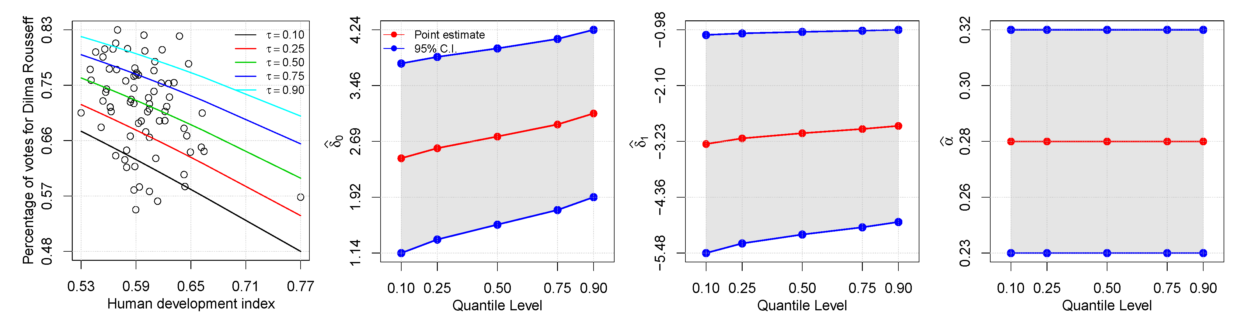
In this first application, the response variable indicates the proportion of voters in the 2014 Brazil presidential election, received by the elected president, Dilma Rousseff, in 74 municipalities of the state of Sergipe. This state is located in the Northeast Region of Brazil and is formed by 75 municipalities. The data set is available in the library baquantreg [53] from R and was considered the human development index (HDI) in 2010 as covariate. We call this set “vote data” and assume the regression structure for ${\mu }_i$ formulated as $\mathrm{logit}\left({\mu }_i\right)={\delta }_0+{\delta }_1{\mathrm{HDI}}_i$, for $i=1,\dots ,74$.

Table 7. ML estimates and SEs of the indicated model, parameter and quantile level ($\tau$) with vote data.

Model	Parameter	Estimate					SE
		$\mathit{\tau }$ Level					$\mathit{\tau }$ Level
		0.10	0.25	0.50	0.75	0.90	0.10	0.25	0.50	0.75	0.90
KUMA	$\alpha$	$12.204$	$12.209$	$12.215$	$12.222$	$12.228$	$1.152$	$1.152$	$1.152$	$1.151$	$1.151$
	${\delta }_0$	$1.717$	$2.153$	$2.649$	$3.158$	$3.629$	$0.462$	$0.529$	$0.612$	$0.702$	$0.786$
	${\delta }_1$	$-2.081$	$-2.425$	$-2.862$	$-3.352$	$-3.835$	$0.764$	$0.877$	$1.015$	$1.161$	$1.296$
LEEG	$\alpha$	$18.176$	$18.183$	$18.190$	$18.198$	$18.207$	$1.825$	$1.825$	$1.825$	$1.826$	$1.826$
	${\delta }_0$	$2.155$	$2.506$	$2.937$	$3.481$	$4.197$	$0.415$	$0.450$	$0.496$	$0.562$	$0.660$
	${\delta }_1$	$-2.708$	$-3.005$	$-3.395$	$-3.924$	$-4.662$	$0.677$	$0.738$	$0.816$	$0.919$	$1.062$
UBS	$\alpha$	$0.279$	$0.279$	$0.279$	$0.279$	$0.279$	$0.023$	$0.023$	$0.023$	$0.023$	$0.023$
	${\delta }_0$	$2.457$	$2.596$	$2.760$	$2.925$	$3.077$	$0.670$	$0.645$	$0.623$	$0.605$	$0.592$
	${\delta }_1$	$-3.281$	$-3.168$	$-3.066$	$-2.978$	$-2.916$	$1.123$	$1.081$	$1.043$	$1.012$	$0.989$
UBURR	$\alpha$	$40.007$	$40.004$	$40.085$	$40.663$	$40.661$	$11.258$	$11.249$	$11.280$	$11.539$	$11.538$
	${\delta }_0$	$1.907$	$2.294$	$2.784$	$3.398$	$4.068$	$0.423$	$0.484$	$0.570$	$0.671$	$0.788$
	${\delta }_1$	$-2.368$	$-2.733$	$-3.184$	$-3.763$	$-4.390$	$0.692$	$0.797$	$0.938$	$1.102$	$1.289$
UCHEN	$\alpha$	$3.712$	$3.712$	$3.712$	$3.712$	$3.712$	$0.335$	$0.335$	$0.335$	$0.334$	$0.334$
	${\delta }_0$	$2.246$	$2.392$	$2.578$	$2.803$	$3.057$	$0.665$	$0.661$	$0.650$	$0.634$	$0.619$
	${\delta }_1$	$-2.939$	$-2.908$	$-2.848$	$-2.766$	$-2.683$	$1.113$	$1.106$	$1.087$	$1.057$	$1.026$
UHN	${\delta }_0$	$0.742$	$1.672$	$2.422$	$2.956$	$3.314$	$1.408$	$1.408$	$1.408$	$1.408$	$1.408$
	${\delta }_1$	$-3.000$	$-3.000$	$-3.000$	$-3.000$	$-3.000$	$2.353$	$2.353$	$2.353$	$2.353$	$2.353$
ULOG	$\alpha$	$5.304$	$5.304$	$5.304$	$5.305$	$5.304$	$0.512$	$0.512$	$0.512$	$0.512$	$0.512$
	${\delta }_0$	$2.506$	$2.713$	$2.921$	$3.127$	$3.335$	$0.566$	$0.564$	$0.563$	$0.563$	$0.564$
	${\delta }_1$	$-3.338$	$-3.338$	$-3.338$	$-3.338$	$-3.338$	$0.939$	$0.939$	$0.939$	$0.939$	$0.939$
>UWEI	$\alpha$	$3.768$	$3.768$	$3.767$	$3.767$	$3.767$	$0.324$	$0.324$	$0.324$	$0.324$	$0.324$
	${\delta }_0$	$2.302$	$2.414$	$2.573$	$2.781$	$3.027$	$0.697$	$0.676$	$0.652$	$0.629$	$0.610$
	${\delta }_1$	$-3.032$	$-2.940$	$-2.835$	$-2.729$	$-2.637$	$1.169$	$1.132$	$1.091$	$1.049$	$1.013$

Where we recall that KUMA: Kumaraswamy, LEEG: log-extended exponential-geometric, UBS: unit Birnbaum–Saunders, UBUR: unit Burr XII, UCHE: unit Chen, UHN: unit half-normal, ULOG: unit logistic, UWEI: unit Weibull.

reports the ML estimates and SEs for the indicated models. Note the difference between the estimates of ${\delta }_0$ and ${\delta }_1$ in the models. The rate of change in the conditional quantile, expressed by the estimated regression coefficients, is illustrated in Figure 3. Observe how the rate of change in the proportion of votes depends on the quantile. As also shown in Figure 3, the first plot on the left, a higher HDI indicates less proportion of votes received by the elected president.

ML estimates for the UBS model parameters can be obtained from the unitBSQuantReg package using the instructions:

install.packages(‘‘remotes’’)
remotes::install_github(‘‘AndrMenezes/unitBSQuantReg’’)
library(unitBSQuantReg)
data(BrazilElection2014, package = ‘‘baquantreg’’)
ind     <- which(BrazilElection2014$UF_name == ‘‘SE’’)
data.se  <- BrazilElection2014[ind, c(‘‘percVotes", ‘‘HDI’’)]
taus    <- c(0.10, 0.25, 0.50, 0.75, 0.90)
fits    <- lapply(taus, function(TAU)
unitBSQuantReg(percVotes ~ HDI, data = data.se, tau = TAU))
lapply(fits, coef)
	  

For the other models, the ML estimates were obtained from the unitquantreg package, which is under development.

Table 8. Values of the Akaike information criterion for the indicated model and quantile level ($\tau$) with vote data.

Model	$\mathit{\tau }$ Level
	0.10	0.25	0.50	0.75	0.90
KUMA	$-186.6585$	$-186.7418$	$-186.8450$	$-186.9566$	$-187.0622$
LEEG	$-181.1746$	$-181.2213$	$-181.2757$	$-181.3365$	$-181.3965$
UBS	$-188.7764$	$-188.7825$	$-188.7883$	$-188.7932$	$-188.7969$
UBUR	$-180.7540$	$-180.7524$	$-180.7513$	$-180.7531$	$-180.7528$
UCHE	$-178.9413$	$-178.9489$	$-178.9513$	$-178.9480$	$-178.9416$
UHN	$-112.5021$	$-112.5021$	$-112.5021$	$-112.5021$	$-112.5021$
ULOG	$-186.1657$	$-186.1657$	$-186.1657$	$-186.1657$	$-186.1657$
UWEI	$-179.3758$	$-179.3678$	$-179.3581$	$-179.3479$	$-179.3385$

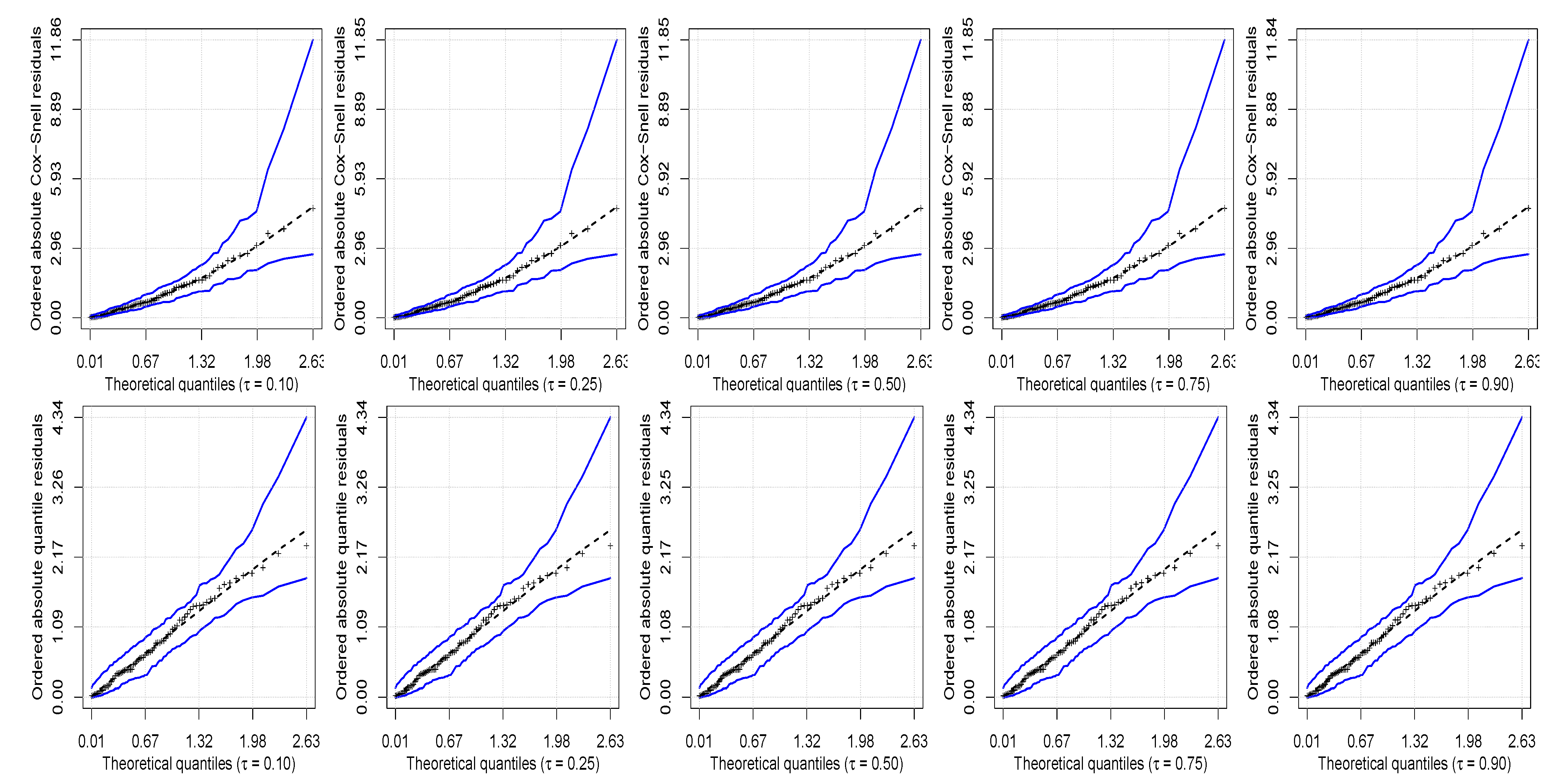
Where we recall that KUMA: Kumaraswamy, LEEG: log-extended exponential-geometric, UBS: unit Birnbaum–Saunders, UBUR: unit Burr XII, UCHE: unit Chen, UHN: unit half-normal, ULOG: unit logistic, UWEI: unit Weibull.

presents the values of the Akaike information criterion used to compare various competing models. These values indicate that the UBS quantile regression model is the best one. This better performance, of course, is not a rule and depends on the data under analysis, but this fact highlights the importance of our new proposal for such data. In order to assess the goodness of fit of the UBS quantile regression model to the vote data, in Figure 4 are shown the half-normal plots with simulated envelopes for the Cox–Snell and randomized quantile residuals. These figures indicate a good fit of the UBS quantile regression model to the $\tau$-th proportion of votes, for $\tau \in (0.10,0.25,0.50,0.75,0.90)$.

6. Empirical Application with Data from Sports Medicine

In this second application, we consider a data set taken from [54], also available at http://www.leg.ufpr.br/doku.php/publications:papercompanions:multquasibeta (accessed on 9 April 2021). These data are related to the body fat percentage, which was measured at five regions: android, arms, gynoid, legs, and trunk. The fat percentages at android, arms, gynoid, legs, and trunk correspond to the five response variables considered in the original study where these data were collected. The data set contains 298 observations and the covariates are: age (in years), body mass index (in kg/m${}^2$), gender (female or male) and IPAQ (sedentary (S), insufficiently active (I), or active (A)). As described in [55], the IPAQ is a questionnaire that allows the estimation of weekly time spent on physical activities of moderate and strong intensity, in different contexts of daily life, such as: housework, leisure, transportation, and work, as well as the time spent in passive activities performed on the seating position.

We analyze the response variable body fat percentage at arms. We call this set as “arm data”. The results of the analyses for the other four responses are available under request from the authors. For the response variable analyzed here, we assume ${\mu }_i$ is given by $\mathrm{logit}\left({\mu }_i\right)={\delta }_0+{\delta }_1{z}_{i1}+{\delta }_2{z}_{i2}+{\delta }_3{z}_{i3}+{\delta }_4{z}_{i4}+{\delta }_5{z}_{i5}$, for $i=1,\cdots ,298$, where $z_{i1}$: age; $z_{i2}$: body mass index; $z_{i3}$: 0 for female, 1 for male; $z_{i4}$: 0 for IPAQ = S, 1 for IPAQ = I; and $z_{i5}$: 0 for IPAQ = S, 1 for IPAQ = A.

Table 9. ML estimates and SEs of the indicated model, parameter and quantile level ($\tau$) with arm data.

Model	Parameter	Estimate					SE
		$\mathit{\tau }$ Level					$\mathit{\tau }$ Level
		0.10	0.25	0.50	0.75	0.90	0.10	0.25	0.50	0.75	0.90
KUMA	$\alpha$	$4.705$	$4.715$	$4.724$	$4.731$	$4.736$	$0.210$	$0.210$	$0.210$	$0.210$	$0.210$
	${\delta }_0$	$-3.071$	$-2.894$	$-2.754$	$-2.658$	$-2.599$	$0.135$	$0.140$	$0.147$	$0.156$	$0.163$
	${\delta }_1$	$0.004$	$0.004$	$0.004$	$0.004$	$0.005$	$0.001$	$0.001$	$0.001$	$0.001$	$0.001$
	${\delta }_2$	$7.291$	$7.721$	$8.226$	$8.743$	$9.210$	$0.551$	$0.577$	$0.609$	$0.644$	$0.676$
	${\delta }_3$	$-0.730$	$-0.771$	$-0.820$	$-0.870$	$-0.915$	$0.033$	$0.035$	$0.037$	$0.039$	$0.041$
	${\delta }_4$	$-0.072$	$-0.074$	$-0.076$	$-0.078$	$-0.078$	$0.047$	$0.050$	$0.054$	$0.057$	$0.060$
	${\delta }_5$	$-0.196$	$-0.206$	$-0.216$	$-0.227$	$-0.236$	$0.047$	$0.050$	$0.053$	$0.056$	$0.060$
LEEG	$\alpha$	$7.587$	$7.609$	$7.629$	$7.648$	$7.671$	$0.375$	$0.375$	$0.375$	$0.375$	$0.374$
	${\delta }_0$	$-3.159$	$-3.056$	$-2.968$	$-2.897$	$-2.850$	$0.142$	$0.147$	$0.154$	$0.163$	$0.175$
	${\delta }_1$	$0.004$	$0.005$	$0.005$	$0.005$	$0.006$	$0.001$	$0.001$	$0.001$	$0.001$	$0.001$
	${\delta }_2$	$8.331$	$8.746$	$9.269$	$9.934$	$10.785$	$0.650$	$0.676$	$0.711$	$0.757$	$0.817$
	${\delta }_3$	$-0.870$	$-0.909$	$-0.957$	$-1.020$	$-1.100$	$0.035$	$0.037$	$0.039$	$0.041$	$0.045$
	${\delta }_4$	$-0.114$	$-0.122$	$-0.131$	$-0.143$	$-0.159$	$0.051$	$0.053$	$0.056$	$0.060$	$0.065$
	${\delta }_5$	$-0.234$	$-0.244$	$-0.257$	$-0.272$	$-0.292$	$0.047$	$0.050$	$0.052$	$0.055$	$0.060$
UBS	$\alpha$	$0.160$	$0.160$	$0.160$	$0.159$	$0.159$	$0.007$	$0.007$	$0.007$	$0.007$	$0.007$
	${\delta }_0$	$-3.394$	$-3.105$	$-2.801$	$-2.522$	$-2.289$	$0.160$	$0.150$	$0.141$	$0.134$	$0.129$
	${\delta }_1$	$0.005$	$0.005$	$0.004$	$0.004$	$0.004$	$0.001$	$0.001$	$0.001$	$0.001$	$0.001$
	${\delta }_2$	$9.525$	$9.045$	$8.581$	$8.161$	$7.820$	$0.705$	$0.666$	$0.629$	$0.596$	$0.572$
	${\delta }_3$	$-1.001$	$-0.947$	$-0.896$	$-0.850$	$-0.813$	$0.040$	$0.038$	$0.035$	$0.033$	$0.032$
	${\delta }_4$	$-0.127$	$-0.122$	$-0.116$	$-0.111$	$-0.108$	$0.053$	$0.051$	$0.048$	$0.046$	$0.044$
	${\delta }_5$	$-0.271$	$-0.256$	$-0.244$	$-0.232$	$-0.223$	$0.052$	$0.049$	$0.047$	$0.044$	$0.042$
UBUR	$\alpha$	$0.453$	$0.457$	$0.459$	$0.461$	$0.463$	$0.043$	$0.043$	$0.043$	$0.043$	$0.043$
	${\delta }_0$	$-1.485$	$-1.109$	$-0.782$	$-0.514$	$-0.283$	$0.496$	$0.257$	$0.098$	$0.030$	$0.109$
	${\delta }_1$	$0.002$	$0.001$	$0.000$	$-0.000$	$-0.000$	$0.006$	$0.003$	$0.001$	$0.000$	$0.001$
	${\delta }_2$	$-0.302$	$-0.003$	$0.045$	$-0.008$	$-0.095$	$2.675$	$1.346$	$0.507$	$0.056$	$0.482$
	${\delta }_3$	$-1.035$	$-0.495$	$-0.182$	$0.019$	$0.168$	$0.225$	$0.102$	$0.037$	$0.019$	$0.044$
	${\delta }_4$	$0.114$	$0.057$	$0.021$	$-0.002$	$-0.020$	$0.186$	$0.095$	$0.036$	$0.004$	$0.034$
	${\delta }_5$	$-0.122$	$-0.072$	$-0.030$	$0.003$	$0.030$	$0.207$	$0.105$	$0.040$	$0.005$	$0.038$
UCHEN	$\alpha$	$1.799$	$1.805$	$1.809$	$1.805$	$1.783$	$0.039$	$0.039$	$0.039$	$0.040$	$0.041$
	${\delta }_0$	$-3.572$	$-3.503$	$-3.396$	$-3.214$	$-2.872$	$0.189$	$0.203$	$0.223$	$0.252$	$0.293$
	${\delta }_1$	$0.005$	$0.006$	$0.007$	$0.007$	$0.008$	$0.002$	$0.002$	$0.002$	$0.002$	$0.002$
	${\delta }_2$	$9.700$	$10.393$	$11.374$	$12.547$	$13.522$	$0.825$	$0.880$	$0.959$	$1.068$	$1.218$
	${\delta }_3$	$-0.962$	$-1.033$	$-1.138$	$-1.265$	$-1.371$	$0.048$	$0.052$	$0.056$	$0.064$	$0.073$
	${\delta }_4$	$-0.120$	$-0.128$	$-0.138$	$-0.144$	$-0.139$	$0.075$	$0.080$	$0.087$	$0.096$	$0.103$
	${\delta }_5$	$-0.329$	$-0.353$	$-0.387$	$-0.428$	$-0.460$	$0.073$	$0.078$	$0.085$	$0.094$	$0.104$
UHN	${\delta }_0$	$-4.854$	$-3.923$	$-3.173$	$-2.639$	$-2.282$	$0.350$	$0.350$	$0.350$	$0.350$	$0.350$
	${\delta }_1$	$0.004$	$0.004$	$0.004$	$0.004$	$0.004$	$0.003$	$0.003$	$0.003$	$0.003$	$0.003$
	${\delta }_2$	$8.754$	$8.754$	$8.755$	$8.754$	$8.755$	$1.533$	$1.534$	$1.533$	$1.531$	$1.533$
	${\delta }_3$	$-0.884$	$-0.884$	$-0.884$	$-0.884$	$-0.884$	$0.086$	$0.086$	$0.086$	$0.086$	$0.086$
	${\delta }_4$	$-0.108$	$-0.108$	$-0.108$	$-0.108$	$-0.108$	$0.126$	$0.126$	$0.126$	$0.126$	$0.126$
	${\delta }_5$	$-0.242$	$-0.242$	$-0.242$	$-0.242$	$-0.242$	$0.122$	$0.122$	$0.122$	$0.122$	$0.122$
ULOG	$\alpha$	$5.821$	$5.821$	$5.821$	$5.821$	$5.821$	$0.282$	$0.282$	$0.282$	$0.282$	$0.282$
	${\delta }_0$	$-3.265$	$-3.076$	$-2.888$	$-2.699$	$-2.510$	$0.146$	$0.145$	$0.145$	$0.145$	$0.145$
	${\delta }_1$	$0.005$	$0.005$	$0.005$	$0.005$	$0.005$	$0.001$	$0.001$	$0.001$	$0.001$	$0.001$
	${\delta }_2$	$8.878$	$8.878$	$8.878$	$8.878$	$8.878$	$0.663$	$0.661$	$0.662$	$0.661$	$0.661$
	${\delta }_3$	$-0.932$	$-0.932$	$-0.932$	$-0.932$	$-0.932$	$0.036$	$0.036$	$0.036$	$0.036$	$0.036$
	${\delta }_4$	$-0.122$	$-0.122$	$-0.122$	$-0.122$	$-0.122$	$0.051$	$0.051$	$0.051$	$0.051$	$0.051$
	${\delta }_5$	$-0.239$	$-0.239$	$-0.239$	$-0.239$	$-0.239$	$0.049$	$0.049$	$0.049$	$0.049$	$0.049$
UWEI	$\alpha$	$5.976$	$5.980$	$5.985$	$5.992$	$6.000$	$0.243$	$0.243$	$0.243$	$0.243$	$0.243$
	${\delta }_0$	$-3.214$	$-2.960$	$-2.640$	$-2.272$	$-1.895$	$0.168$	$0.159$	$0.148$	$0.138$	$0.130$
	${\delta }_1$	$0.006$	$0.005$	$0.005$	$0.005$	$0.004$	$0.001$	$0.001$	$0.001$	$0.001$	$0.001$
	${\delta }_2$	$8.592$	$8.201$	$7.729$	$7.218$	$6.735$	$0.729$	$0.691$	$0.647$	$0.600$	$0.556$
	${\delta }_3$	$-0.966$	$-0.919$	$-0.863$	$-0.803$	$-0.746$	$0.043$	$0.040$	$0.037$	$0.035$	$0.032$
	${\delta }_4$	$-0.131$	$-0.127$	$-0.121$	$-0.115$	$-0.109$	$0.055$	$0.053$	$0.050$	$0.047$	$0.044$
	${\delta }_5$	$-0.355$	$-0.339$	$-0.319$	$-0.298$	$-0.277$	$0.055$	$0.053$	$0.050$	$0.047$	$0.043$

Where we recall that KUMA: Kumaraswamy, LEEG: log-extended exponential-geometric, UBS: unit Birnbaum–Saunders, UBUR: unit Burr XII, UCHE: unit Chen, UHN: unit half-normal, ULOG: unit logistic, UWEI: unit Weibull.

reports the ML estimates and SEs for the indicated models. Note the difference between the estimates of ${\delta }_j$, for $j=0,1,\cdots ,5$, in the models. The rate of change in the conditional quantile, expressed by the estimated regression coefficients, is illustrated in Figure 5. Note how the rate of change in body fat percentage at arms depends on the quantile.

Table 10. Values of the Akaike information criterion for the indicated model and quantile level ($\tau$) with arm data.

Model	$\mathit{\tau }$ Level
	0.10	0.25	0.50	0.75	0.90
KUMA	$-839.660$	$-842.224$	$-845.030$	$-847.657$	$-849.813$
LEEG	$-846.433$	$-849.810$	$-853.814$	$-858.493$	$-863.789$
UBS	$-905.942$	$-907.590$	$-909.332$	$-910.964$	$-912.330$
UBUR	$-466.813$	$-467.464$	$-467.982$	$-468.339$	$-468.586$
UCHEN	$-690.483$	$-691.734$	$-691.722$	$-687.523$	$-676.318$
UHN	$-546.283$	$-546.283$	$-546.283$	$-546.283$	$-546.283$
ULOG	$-888.401$	$-888.401$	$-888.401$	$-888.401$	$-888.401$
UWEI	$-838.151$	$-839.364$	$-840.932$	$-842.757$	$-844.603$

Where we recall that KUMA: Kumaraswamy, LEEG: log-extended exponential-geometric, UBS: unit Birnbaum–Saunders, UBUR: unit Burr XII, UCHE: unit Chen, UHN: unit half-normal, ULOG: unit logistic, UWEI: unit Weibull.

presents the values of the Akaike information criterion used to compare various models. These values indicate that the UBS quantile regression model is the best one. In order to assess if this model fits the data well, in Figure 6 are shown the half-normal plots with simulated envelopes for the residuals. This figure displays a good fit of the UBS quantile regression model to the $\tau$-th percentage of body fat at arms, for $\tau \in (0.10,0.25,0.50,0.75,0.90)$.

7. Conclusions, Limitations and Future Investigation

Although the quantile regression methodology appeared in 1978 [34], few works consider it from a strictly parametric point of view. Some of these recently published works used distributions for responses restricted to the zero-one interval.

In this paper, we extended the unit Birnbaum–Saunders distribution by parameterizing its scale parameter in terms of a quantile that can depend on covariates. This extension employed a quantile parameterization that permitted us to state a setting mimicking the generalized linear models, giving wide flexibility in the formulation.

We estimated the model parameter with the maximum likelihood method and used Cox–Snell and randomized quantile residuals to assess the adequacy of our formulation to the data, as well as the Akaike information criterion for model selection.

We conducted a Monte Carlo simulation study to empirically evaluate the statistical performance of the maximum likelihood estimators of the unit Birnbaum–Saunders quantile regression parameters. We also studied coverage probabilities of the confidence intervals of the corresponding parameters based on the asymptotic normality of these estimators. This simulation study reported the good statistical performance of such estimators.

Two data analyses were conducted related to political sciences and sports medicine with seven competing models to the unit Birnbaum–Saunders quantile regression. Both of these analyses reported a suitable performance of the new regression quantile model and superior to all of the competing models, giving evidence that the unit Birnbaum–Saunders distribution is an excellent alternative for quantile modeling and for dealing with bounded data into the unit interval. Such results reported that the unit Birnbaum–Saunders quantile regression model may be a new setting for analyzing this type of data. The new approach may be a good addition to the tools of statisticians and diverse practitioners interested in the modeling of quantiles.

A limitation of our approach is that the explanatory variables may condition quantiles and also the shape parameter. Thus, the effect of this parameter is a topic to be studied in a future work based on the line presented in [56,57] when jointly modeling two parameters. Other topics of future research are related to studying how multivariate, spatial, temporal structures could be added into the quantile regression framework [58,59,60,61]. In addition, Tobit and Cobb-Douglas type frameworks may be analyzed in the thematic of this investigation [62,63]. Moreover, censored observation might be studied in the present context [64].

The authors are working on these and other issues associated with the present investigation and the corresponding findings are expected to be reported in future works.

References

- Mazucheli, J.; Menezes, A.F.B.; Dey, S. The unit Birnbaum-Saunders distribution with applications. Chil. J. Stat. 2018, 9, 47–57. [Google Scholar]
- Mousa, A.M.; El-Sheikh, A.A.; Abdel-Fattah, M.A. A gamma regression for bounded continuous variables. Adv. Appl. Stat. 2016, 49, 305–326. [Google Scholar] [CrossRef]
- Mazucheli, J.; Menezes, A.F.; Dey, S. Unit-Gompertz distribution with applications. Statistica 2019, 79, 25–43. [Google Scholar]
- Ghitany, M.E.; Mazucheli, J.; Menezes, A.; Alqallaf, F. The unit inverse Gaussian distribution: A new alternative to two-parameter distributions on the unit interval. Commun. Stat. Theory Methods 2019, 48, 3423–3438. [Google Scholar] [CrossRef]
- Mazucheli, J.; Menezes, A.F.B.; Chakraborty, S. On the one parameter unit Lindley distribution and its associated regression model for proportion data. J. Appl. Stat. 2019, 46, 700–714. [Google Scholar] [CrossRef] [Green Version]
- Mazucheli, J.; Bapat, S.R.; Menezes, A.F.B. A new one-parameter unit Lindley distribution. Chil. J. Stat. 2019, 11, 53–67. [Google Scholar]
- Mazucheli, J.; Menezes, A.F.B.; Ghitany, M.E. The unit Weibull distribution and associated inference. J. Appl. Probab. Stat. 2018, 13, 1–22. [Google Scholar]
- Mazucheli, J.; Menezes, A.F.B.; Fernandes, L.B.; de Oliveira, R.P.; Ghitany, M.E. The unit Weibull distribution as an alternative to the Kumaraswamy distribution for the modeling of quantiles conditional on covariates. J. Appl. Stat. 2020, 47, 954–974. [Google Scholar] [CrossRef]
- Menezes, A.F.B.; Mazucheli, J.; Bourguignon, M. A parametric quantile regression approach for modelling zero-or-one inflated double bounded data. Biometr. J. 2021, 63, 841–858. [Google Scholar] [CrossRef] [PubMed]
- Figueroa-Zuniga, J.I.; Niklitschek, S.; Leiva, V.; Liu, S. Modeling heavy-tailed bounded data by the trapezoidal beta distribution with applications. Revstat 2021, in press. [Google Scholar]
- Kieschnick, R.; McCullough, B.D. Regression analysis of variates observed on (0, 1): Percentages, proportions and fractions. Stat. Model. 2003, 3, 193–213. [Google Scholar] [CrossRef] [Green Version]
- Smithson, M.; Verkuilen, J. A better lemon squeezer? Maximum-likelihood regression with beta-distributed dependent variables. Psychol. Methods 2006, 11, 54–71. [Google Scholar] [CrossRef] [Green Version]
- Altun, E.; El-Morshedy, M.; Eliwa, M.S. A new regression model for bounded response variable: An alternative to the beta and unit Lindley regression models. PLoS ONE 2021, 16, 1–15. [Google Scholar] [CrossRef] [PubMed]
- Jodrá, P. A bounded distribution derived from the shifted Gompertz law. J. King Saud Univ. Sci. 2020, 32, 523–536. [Google Scholar] [CrossRef]
- Ferrari, S.; Cribari Neto, F. Beta regression for modelling rates and proportions. J. Appl. Stat. 2004, 31, 799–815. [Google Scholar] [CrossRef]
- Bayes, C.L.; Bazán, J.L.; García, C. A new robust regression model for proportions. Bayesian Anal. 2012, 7, 841–866. [Google Scholar] [CrossRef]
- Gómez-Déniz, E.; Sordo, M.A.; Calderín-Ojeda, E. The log-Lindley distribution as an alternative to the beta regression model with applications in insurance. Insur. Math. Econ. 2014, 54, 49–57. [Google Scholar] [CrossRef]
- Altun, E. The log-weighted exponential regression model: Alternative to the beta regression model. Commun. Stat. Theory Methods 2019, 1–16. [Google Scholar] [CrossRef]
- Bonat, W.H.; Petterle, R.R.; Hinde, J.; Demétrio, C.G.B. Flexible quasi-beta regression models for continuous bounded data. Stat. Model. 2019, 19, 617–633. [Google Scholar] [CrossRef]
- Song, P.X.K.; Tan, M. Marginal models for longitudinal continuous proportional data. Biometrics 2000, 56, 496–502. [Google Scholar] [CrossRef]
- Altun, E.; Cordeiro, G.M. The unit improved second-degree Lindley distribution: Inference and regression modeling. Comput. Stat. 2020, 35, 259–279. [Google Scholar] [CrossRef]
- Zhou, H.; Huang, X.; For the Alzheimer’s Disease Neuroimaging Initiative. Parametric mode regression for bounded responses. Biometr. J. 2020, 62, 1791–1809. [Google Scholar] [CrossRef] [PubMed]
- Menezes, A.F.B.; Mazucheli, J.; Chakraborty, S. A collection of parametric modal regression models for bounded data. J. Biopharm. Stat. 2021, accepted. [Google Scholar]
- Chahuan-Jimenez, K.; Rubilar, R.; de la Fuente-Mella, H.; Leiva, V. Breakpoint analysis for the COVID-19 pandemic and its effect on the stock markets. Entropy 2021, 32, 100. [Google Scholar] [CrossRef] [PubMed]
- Korkmaz, M.Ç.; Chesneau, C.; Korkmaz, Z.S. On the arcsecant hyperbolic normal distribution. Properties, quantile regression modeling and applications. Symmetry 2021, 13, 117. [Google Scholar] [CrossRef]
- Lemonte, A.J.; Moreno-Arenas, G. On a heavy-tailed parametric quantile regression model for limited range response variables. Comput. Stat. 2020, 35, 379–398. [Google Scholar] [CrossRef]
- Mitnik, P.A.; Baek, S. The Kumaraswamy distribution: Median-dispersion re-parameterizations for regression modeling and simulation-based estimation. Stat. Pap. 2013, 54, 177–192. [Google Scholar] [CrossRef]
- Jodrá, P.; Jiménez-Gamero, M.D. A quantile regression model for bounded responses based on the exponential-geometric distribution. Revstat 2020, 4, 415–436. [Google Scholar]
- Paz, R.F.; Balakrishnan, N.; Bazán, J.L. L-logistic regression models: Prior sensitivity analysis, robustness to outliers and applications. Braz. J. Prob. Stat. 2019, 33, 455–479. [Google Scholar]
- Cancho, V.G.; Bazán, J.L.; Dey, D.K. A new class of regression for a bounded response with application in the incidence rate of colorectal cancer. Stat. Methods Med. Res. 2020, 29, 2015–2033. [Google Scholar] [CrossRef]
- Korkmaz, M.Ç.; Emrah, A.; Chesneau, C.; Yousof, H.M. On the unit Chen distribution with associated quantile regression and applications. Int. J. Environ. Res. Public Health 2019, 16, 2748. [Google Scholar]
- Bakouch, H.S.; Nik, A.S.; Asgharzadeh, A.; Salinas, H.S. A flexible probability model for proportion data: Unit-half-normal distribution. Commun. Stat. Case Stud. Data Anal. Appl. 2021, in press. [Google Scholar] [CrossRef]
- Korkmaz, M.Ç.; Chesneau, C. On the unit Burr-XII distribution with the quantile regression modeling and applications. Comput. Appl. Math. 2021, 40, 1–29. [Google Scholar] [CrossRef]
- Koenker, R.; Basset, G. Regression Quantiles. Econometrica 1978, 46, 33–50. [Google Scholar] [CrossRef]
- Birnbaum, Z.W.; Saunders, S.C. A new family of life distributions. J. Appl. Prob. 1969, 6, 319–327. [Google Scholar] [CrossRef]
- Balakrishnan, N.; Gupta, R.C.; Kundu, D.; Leiva, V.; Sanhueza, A. On some mixture models based on the Birnbaum-Saunders distribution and associated inference. J. Stat. Plan. Inference 2011, 141, 2175–2190. [Google Scholar] [CrossRef]
- Patriota, A.G. On scale mixture Birnbaum-Saunders distributions. J. Stat. Plan. Inference 2012, 142, 2221–2226. [Google Scholar] [CrossRef]
- Lemonte, A.J. A note on the Fisher information matrix of the Birnbaum-Saunders distribution. J. Stat. Theory Appl. 2016, 15, 196–205. [Google Scholar]
- Kundu, D.; Kannan, N.; Balakrishnan, N. On the hazard function of Birnbaum-Saunders distribution and associated inference. Comput. Stat. Data Anal. 2008, 52, 2692–2702. [Google Scholar] [CrossRef] [Green Version]
- Rieck, J.R.; Nedelman, J.R. A log-linear model for the Birnbaum-Saunders distribution. Technometrics 1991, 33, 51–60. [Google Scholar]
- Lemonte, A.J. A log-Birnbaum-Saunders regression model with asymmetric errors. J. Stat. Comput. Simul. 2012, 82, 1775–1787. [Google Scholar] [CrossRef] [Green Version]
- Sánchez, L.; Leiva, V.; Galea, M.; Saulo, H. Birnbaum-Saunders quantile regression and its diagnostics with application to economic data. Appl. Stochastic Models Bus. Ind. 2021, 37, 53–73. [Google Scholar] [CrossRef]
- Leiva, V.; Sanchez, L.; Galea, M.; Saulo, H. Global and local diagnostic analytics for a geostatistical model based on a new approach to quantile regression. Stoch. Environ. Res. Risk Assess. 2020, 34, 1457–1471. [Google Scholar] [CrossRef]
- Sánchez, L.; Leiva, V.; Galea, M.; Saulo, H. Birnbaum–Saunders quantile regression models with application to spatial data. Mathematics 2021, 8, 1000. [Google Scholar] [CrossRef]
- Saulo, H.; Dasilva, A.; Leiva, V.; Sanchez, L.; de la Fuente-Mella, H. Log-symmetric quantile regression models. Stat. Neerlandica 2021, in press. [Google Scholar] [CrossRef]
- Koenker, R.; Machado, J.A.F. Goodness of fit and related inference processes for quantile regression. J. Am. Stat. Assoc. 1999, 94, 1296–1310. [Google Scholar] [CrossRef]
- Bayes, C.L.; Bazán, J.L.; Castro, M. A quantile parametric mixed regression model for bounded response variables. Stat. Interface 2017, 10, 483–493. [Google Scholar] [CrossRef]
- Rodrigues, J.; Bazán, J.L.; Suzuki, A.K. A flexible procedure for formulating probability distributions on the unit interval with applications. Commun. Stat. Theory Methods 2020, 49, 738–754. [Google Scholar] [CrossRef]
- Smithson, M.; Shou, Y. CDF-quantile distributions for modelling random variables on the unit interval. Br. J. Math. Stat. Psychol. 2017, 70, 412–438. [Google Scholar] [CrossRef]
- Noufaily, A.; Jones, M.C. Parametric quantile regression based on the generalized gamma distribution. J. R. Stat. C 2013, 62, 723–740. [Google Scholar] [CrossRef]
- Gallardo, D.I.; Gómez-Déniz, E.; Gómez, H.W. Discrete generalized half normal distribution with applications in quantile regression. SORT 2020, 44, 265–284. [Google Scholar]
- Lindsay, B.G.; Li, B. On second-order optimality of the observed Fisher information. Ann. Stat. 1997, 25, 2172–2199. [Google Scholar] [CrossRef]
- Santos, B. Baquantreg: Bayesian Quantile Regression Methods. R Package Version 0.1. 2015. Available online: https://rdrr.io/github/brsantos/baquantreg/ (accessed on 9 April 2021).
- Petterle, R.R.; Bonat, W.H.; Scarpin, C.T.; Jonasson, T.; Borba, V.Z.C. Multivariate quasi–beta regression models for continuous bounded data. Int. J. Biostat. 2020, 1, 1–15. [Google Scholar] [CrossRef]
- Benedetti, T.R.B.; Antunes, P.C.; Rodriguez–Añez, C.R.; Mazo, G.Z.; Petroski, E.L. Reproducibility and validity of the International Physical Activity Questionnaire (IPAQ) in elderly men. Rev. Bras. Med. Esporte 2007, 13, 11–16. [Google Scholar] [CrossRef]
- Santos-Neto, M.; Cysneiros, F.J.A.; Leiva, V.; Barros, M. Reparameterized Birnbaum–Saunders regression models with varying precision. Electronic J. Stat. 2016, 10, 2825–2855. [Google Scholar] [CrossRef]
- Ventura, M.; Saulo, H.; Leiva, V.; Monsueto, S. Log-symmetric regression models: Information criteria, application to movie business and industry data with economic implications. Appl. Stoch. Models Bus. Ind. 2019, 35, 963–977. [Google Scholar] [CrossRef]
- Aykroyd, R.G.; Leiva, V.; Marchant, C. Multivariate Birnbaum–Saunders distributions: Modelling and applications. Risks 2018, 6, 21. [Google Scholar] [CrossRef] [Green Version]
- Garcia-Papani, F.; Uribe-Opazo, M.A.; Leiva, V.; Aykroyd, R.G. Birnbaum–Saunders spatial modelling and diagnostics applied to agricultural engineering data. Stochastic Environ. Res. Risk Assess. 2017, 31, 105–124. [Google Scholar] [CrossRef] [Green Version]
- Leiva, V.; Saulo, H.; Souza, R.; Aykroyd, R.G.; Vila, R. A new BISARMA time series model for forecasting mortality using weather and particulate matter data. J. Forecast. 2021, 40, 346–364. [Google Scholar] [CrossRef]
- Giraldo, R.; Herrera, L.; Leiva, V. Cokriging prediction using as secondary variable a functional random field with application in environmental pollution. Mathematics 2020, 8, 1305. [Google Scholar] [CrossRef]
- de la Fuente-Mella, H.; Rojas Fuentes, J.L.; Leiva, V. Econometric modeling of productivity and technical efficiency in the Chilean manufacturing industry. Comput. Ind. Eng. 2020, 139, 105793. [Google Scholar] [CrossRef]
- Martinez-Florez, G.; Leiva, V.; Gomez-Deniz, E.; Marchant, C. A family of skew-normal distributions for modeling proportions and rates with zeros/ones excess. Symmetry 2020, 12, 1439. [Google Scholar] [CrossRef]
- Leao, J.; Leiva, V.; Saulo, H.; Tomazella, V. A survival model with Birnbaum–Saunders frailty for uncensored and censored cancer data. Braz. J. Probab. Stat. 2018, 32, 707–729. [Google Scholar] [CrossRef] [Green Version]
- Kumaraswamy, P. A generalized probability density function for double-bounded random processes. J. Hydrol. 1980, 46, 79–88. [Google Scholar] [CrossRef]
Figure 1.
PDFs of the unit UBS distribution for the indicated values of , and .
Figure 2.
Behaviors of the mean, variance, coefficient of skewness and coefficient of kurtosis for the indicated values of and in function of .
Figure 3.
Quantile regression fit plot (left) and estimated quantile process plots for (center left), (center right) and (right) with vote data.
Figure 4.
Half-normal plots with envelopes of Cox–Snell (first row) and randomized quantile (second row) residuals for the indicated quantile level with vote data.
Figure 5.
Estimated quantile process plot for the indicated , with , and (second row right) with arm data.
Figure 6.
Half-normal plots with envelopes of Cox–Snell (first row) and randomized quantile (second row) residuals for the indicated quantile level with arm data.