
X-SDD: A New Benchmark for Hot Rolled Steel Strip Surface Defects Detection


College of Information Science and Engineering, Northeastern University, Shenyang 110819, China
*
Author to whom correspondence should be addressed.
†
These authors contributed equally to this work.
Symmetry 2021, 13(4), 706; https://doi.org/10.3390/sym13040706
Submission received: 18 March 2021
/
Revised: 9 April 2021
/
Accepted: 15 April 2021
/
Published: 17 April 2021
Abstract
:It is important to accurately classify the defects in hot rolled steel strip since the detection of defects in hot rolled steel strip is closely related to the quality of the final product. The lack of actual hot-rolled strip defect data sets currently limits further research on the classification of hot-rolled strip defects to some extent. In real production, the convolutional neural network (CNN)-based algorithm has some difficulties, for example, the algorithm is not particularly accurate in classifying some uncommon defects. Therefore, further research is needed on how to apply deep learning to the actual detection of defects on the surface of hot rolled steel strip. In this paper, we proposed a hot rolled steel strip defect dataset called Xsteel surface defect dataset (X-SDD) which contains seven typical types of hot rolled strip defects with a total of 1360 defect images. Compared with the six defect types of the commonly used NEU surface defect database (NEU-CLS), our proposed X-SDD contains more types. Then, we adopt the newly proposed RepVGG algorithm and combine it with the spatial attention (SA) mechanism to verify the effect on the X-SDD. Finally, we apply multiple algorithms to test on our proposed X-SDD to provide the corresponding benchmarks. The test results show that our algorithm achieves an accuracy of 95.10% on the testset, which exceeds other comparable algorithms by a large margin. Meanwhile, our algorithm achieves the best results in Macro-Precision, Macro-Recall and Macro-F1-score metrics.
1. Introduction
Hot rolled steel strip has important applications in areas such as automotive [1], appliance manufacturing, bridges [2], electric motors which have great use in industry and daily life. The surface quality of the steel strip is of paramount importance to the final product, therefore surface defects in the steel strip must be strictly controlled. The surface quality of strip steel can be affected by several factors [3,4,5], although the number of strip surface defects generated can be reduced to some extent by a variety of reasonable control methods, until now the surface of the steel strip inevitably exit different types of defects, e.g., slag inclusion, red iron and surface scratches. These various surface defects of hot rolled steel strip have different effects on the production quality, therefore, it is necessary to classify the surface defects of hot rolled steel strip in order to better reduce their adverse effects.
Existing hot rolled strip lines are usually equipped with surface defect detection systems that can detect defects on the strip surface [6]; however, unfortunately, the system is less accurate in classifying defects. Existing surface inspection systems for hot rolled steel strip often have a classification accuracy of about 85% according to the systems technical manual; however, in the actual process of operation, due to some reasons, the actual performance of the system did not reach the expected results according to the report of the relevant quality inspectors. This case prevents the system from completely replacing manual work and only serves as an aid. A steel mill has recognized the shortcomings of the system’s classification accuracy and is now trying to use more advanced algorithms to improve the classification accuracy of defects.
The practical steps for detecting surface defects in existing hot rolled steel strip in a steel mill are as follows: Firstly, the hot rolled steel strip surface defect detection system performs the initial detection as well as classification of surface defects on hot rolled steel strips. Secondly, the defects found by the system are inspected by quality control personnel and the steel strip is blocked according to the type and degree of its surface defects. As the hot rolled steel strip passes through the surface inspection system very quickly, the quality inspector needs to make a judgement on whether to block the steel strip coil within a few minutes. After the faulty steel strip coils have been blocked, another group of quality inspectors will make a secondary detection of the blocked coils. Then these quality inspectors will give subsequent units some instructions such as cutting out, polishing and taking a sample. Finally, the subsequent units, e.g., smoothing units and trimming units, will treat the defects appropriately according to the instructions. The resulting steel strip coil is shown in Figure 1.
The aforementioned method of detecting defects in hot rolled steel strip is much more efficient than a purely manual method for a steel strip surface defect detection system is used to reduce the workload of quality inspectors. However, it has the following shortcomings: (1) The quality inspectors have to determine within a few minutes whether the steel strip coil needs to be blocked based on the defects given by the hot rolled steel strip surface defect detection system, which inevitably leads to misjudgements in a panic due to time constraints [7]. (2) Due to the round-the-clock operation of the hot-rolled strip line, quality inspectors are often required to work at night, which may have a negative impact on their health [8]. (3) The current defect classification requires quality inspectors to stare at the computer screen for a long time, such boring work is likely to cause visual and brain fatigue which in turn leads to errors.
Once a quality inspector makes a mistake such as a surface defects of the hot rolled steel strip that should have been treated is let go, the following undesirable consequences may result: (1) Some steel strip surface defects are so severe that they need to be removed during the flattening stage. If these defects are not treated, the strip may break during the subsequent cold rolling process, which can be very troublesome to deal with. Since it takes maintenance personnel one to two hours to handle a broken steel strip, the line has to be shut down during this time, thus affecting subsequent production and reducing steel strip output. (2) Some defects on the surface of the steel strip, if left untreated, will force the finished strip coil to be sold separately at a reduced price because it cannot meet the customer’s requirements. This will inevitably have a negative impact on the benefits of the steel mill.
Therefore, improving the accuracy of the classification of surface defects in hot rolled strip to reduce the extent of manual intervention in defect classification can bring significant economic and social benefits. On the one hand, the quality inspectors can avoid heavy night work, which is good for their health. On the other hand, the errors caused by fatigue and other factors of the quality inspectors will be greatly reduced, thus improving the output and quality of the strip steel and bringing greater benefits to the steel mill.
In summary, the contributions of this paper are shown below:
- We propose a hot-rolled steel strip defect dataset for strip surface defect classification, which is named Xsteel Surface Defect Dataset (X-SDD) and contains seven typical hot-rolled steel strip defects with 1360 defect images;
- We apply RepVGG algorithms and spatial attention (RepVGG+SA) to classify the defects of X-SDD we proposed. The classification accuracy, Macro-Recall, Macro-Precision, and Macro-F1-score of the testset are 95.10%, 93.92%, 95.16%, 93.25%, respectively;
- We employ a variety of different algorithms such as ResNet, VGG, MobileNet etc. to verify the effectiveness of the dataset X-SDD and algorithm RepVGG+SA. The comparison of test results demonstrate that the RepVGG+SA we proposed achieves the best performance in several metrics.
2. Related Work
The earliest defect detection method of steel strip is totally dependent on manual visual inspection method which cannot meet the requirement of real-time. In addition, manual visual inspection also has the disadvantages of labor intensity, missed inspection, mis-inspection, poor working environment and easy to cause injuries to quality inspectors. With the increase in production speed, it is difficult to achieve complete detection by manual visual inspection. Therefore, it gradually evolved into random inspection, i.e., randomly select a certain percentage of completed production of steel coils, and then open a few meters on the uncoiler to check whether there are defects. Since the sampling inspection method cannot achieve a comprehensive inspection of steel coils, it has been largely replaced by machine vision inspection systems.
The machine vision inspection system is shown in Figure 2 and more detailed information can be found in [3]. In actual production, such vision inspection systems for metal surfaces have been used in many applications and have achieved certain results [9,10,11]. Detection devices generally include industrial cameras, light sources, protection devices, etc. Since both the upper and lower surfaces of the steel strip need to be inspected, the detection devices are installed symmetrically on the top and bottom surface of the steel strip. If the detection devices cannot be installed symmetrically for some reasons on site; then two different sets of detection algorithms are required for detection. In this case, although the detection results can be basically the same as if the detection devices were installed symmetrically, this undoubtedly increases the workload. Therefore, in practice, the symmetrical installation of the detection devices should be ensured as much as possible. The detection range of industrial cameras needs to cover the whole steel strip, so it is necessary to arrange an appropriate number of cameras according to the width of the steel strip. In general, seven cameras are sufficient to cover the entire steel strip surface. If the distance between the camera and the steel strip is increased, the camera’s observation range of the steel strip surface becomes larger, so the number of cameras can be reduced. The speed of the strip moving on the conveyor rollers can reach 400 m/min, so the industrial camera needs to shoot at high speed to meet the real-time requirements. Since the exposure time is relatively short when the camera is shooting at high speed, proper fill light is essential in order to make enough light enter the camera in a short time. The images captured by the industrial cameras are transmitted via optical fiber to the server, where the relevant algorithms on the server process the images and then display the processed images on the console panel. The algorithms in the server are the key to this, and in general, machine learning algorithms are mainly used.
In recent years, many researchers have carried out meaningful research work on the detection of steel strip surface defects on using machine learning algorithms. Refs. [12,13,14] described the use of the k-nearest neighbor algorithm for steel strip defect detection. Ref. [15] used back propagation (BP) neural network algorithm to steel strip surface defect classification. Ref. [16] used random forests (RF) and support vector machines (SVMs) to achieve multiple classification of steel strip surface defects. Refs. [17,18,19,20,21] described the effectiveness of various improved versions of SVMs for the detection of steel strip surface defects. Ref. [22] applied the LBP algorithm to the recognition of steel strip surface defects. Although the above solutions using machine learning can achieve certain results, there are still some shortcomings. On the one hand, traditional machine learning methods often require feature extraction first, which leads to algorithms whose results will be limited by the results of feature extraction. On the other hand, the classification accuracy of machine learning is often not particularly high. For these reasons, since 2014, with the advancement of deep learning technology, more and more scholars have employed deep learnings for steel strip surface defects identification and classification.
Due to the powerful feature extraction capability of CNN, the use of CNN-based classification networks has now become the most commonly used model for steel strip surface defect classification. CNN networks generally use convolutional and pooling layers for feature extraction, which is efficient in the way that feature extraction does not need to be performed manually. In general, existing strip surface defect classification networks tend to use off-the-shelf deep learning network structures and their various variants, including AlexNet [23], VGGNet [24], GoogleNet [25], ResNet [26], DenseNet [27], SENet [28], ShuffleNet [29] and MobileNet [30], etc. Compared with traditional algorithms such as machine learning, deep learning algorithms have higher accuracy; however, deep learning often requires a larger amount of data. The lack of high-quality steel strip defect datasets makes the effectiveness of deep learning in steel strip defect classification somewhat limited.
Currently, the NEU surface defect database (NEU-CLS) [31] is a common dataset for steel strip defect classification. Many high-level studies have been conducted based on this dataset, for example, [32,33,34,35,36]. Although NEU-CLS meets the needs of scholars to a certain extent; the effectiveness of the algorithm can be better verified with the complement of other datasets, and the experimental results on multiple datasets will be more convincing. In addition, NEU-CLS contains a total of six types of defects and each type is balanced, all containing 300 images. In practice, the frequency of different types of defects often varies, so researchers need a dataset with varying numbers of each type of defect to conduct relevant studies.
3. Introduction to Datasets
3.1. The Xsteel Surface Defect Dataset
The dataset of surface defects of hot rolled steel strip presented in this paper are from the hot rolled steel strip field where the acquisition is similar to that shown in Figure 2. The resolution of each defect image is pixels, and the image is in 3-channel JPG format. The dataset contains seven types of 1360 defect images, including 238 slag inclusions (abbreviated as “inclusion”), 397 red iron sheet, 122 iron sheet ash, 134 surface scratches (abbreviated as “scratches”), 63 oxide scale of plate system, 203 finishing roll printing and 203 oxide scale of temperature system. We chose the above seven defects to put in the dataset because they are relatively common and fairly representative. In the next part of this article, we will describe in detail about the style and causes of each type of defect.
Inclusions defects are shown in Figure 3a and usually occur during the slab continuous casting process. They are formed due to the presence of large amounts of inclusions caused by slag entrapment in the slab, which are extended and exposed during the subsequent hot rolling process. Inclusions defects are characterized by a visible black non-metallic substance that has a distinct color difference from the surrounding metal. Steel strips with severe slagging defects usually need to be cut off, while steel strips with minor slagging defects can sometimes be removed by manual polishing.
The defects of red iron sheet are shown in Figure 3b, which are common in special steel grades. It is mainly caused by high silicon content in steel and high heating temperature of slab. Its characteristics are: generally reddish brown, dot, strip or flake, distributed in the whole strip. There are obvious pits in some positions after pickling, and the thicker the steel strip size is, the more serious the defects are. The defects of red iron sheet can be reduced by properly increasing the coiling tension, reducing the gap of each layer of steel coil after coiling and reducing the amount of air entering.
The Iron sheet ash defect is shown in Figure 3c, which mostly occurs in the head and tail part of the steel strip. The cause of this defect is that after a long period of production, the surface of the rolling mill equipment accumulates a large amount of metal dust, water, oil and other substances, and when these substances accumulate to a certain extent, they fall onto the surface of the rolled parts and become embedded in them during the subsequent rolling process. Its appearance is characterized by a comet-shaped, visually observable embedded metal particles and black oil residue material.
The scratches are shown in Figure 3d, which generally appears on the lower surface of the steel strip, and the full length and width are randomly distributed. The reason for the formation of this defect is the hot rolling area with projections, or dead rolls, passive rolls and stel strip surface friction. Its appearance is characterized by: defects in the steel strip surface in the form of straight lines and grooves.
The oxide scale of plate system is shown in Figure 3e. The reason for the formation of this defect is: in the high temperature and high speed rolling process, due to the passive rotation of the roller table, dead roll of the roller table, bending deformation of the roller table, wear and tear of the roller surface, the surface of the rolled piece is damaged, and the iron oxide particles are accumulated in the damaged place, which are rolled into the rolled piece in the subsequent rolling deformation process. Its appearance features are: the defect position is basically fixed, and the appearance is similar to scratch and contusion.
As shown in Figure 3f, the finishing roll printing generally occurs on the edge with width less than 1200 mm and is continuously distributed along the length direction. The formation principle is that there is slippage between the work roll and the support roll, resulting in dot and short strip damage on the surface of the work roll. Its appearance features are as follows: it is dot shaped and short strip-shaped pits, densely distributed at the same location.
The oxide scale of temperature system is shown in Figure 3g; its formation is complicated and may be caused by the following: (1) unreasonable rolling schedule arrangement, such as arranging plates with high surface requirements at the later stage of rolling schedule; (2) high carbon content in steel strip, which makes the grain structure of steel more loose; (3) improper use of stand water; (4) too high temperature control in rough rolling; (5) lower surface temperature of steel stripis higher than upper surface; (6) the rack undergoes intense oxidation before the strip goes through the finishing roll. Its appearance is characterized by loose or loose sand [37].
3.2. The Comparison between Xsteel Surface Defect Dataset and NEU Surface Defect Database
The NEU-CLS was collected from hot rolling site whose defect types included inclusion, scratch, pressed oxide scale, crack, pitting and plaque. Figure 4 shows some examples of defects on NEU-CLS. It can be seen from the figure that the defects on X-SDD are different from those on NEU-CLS in morphology. The NEU-CLS contains six types of defects, while the X-SDD we proposed contains seven types of defects.
The NEU-CLS contains 300 images per defect type, but the number of defects contained in each defect category of our proposed X-SDD varies considerably. The pie chart of various types of defects is shown in Figure 5, where the total number of the defects are 1360. From the pie chart, we can see the differences in the number of different types of defects for the range of various defects is different in actual production. For example, defects such as red iron sheet may be widely distributed on individual steel coils, so a large number of samples can be collected; while defects such as iron oxide scale of plate system are easier to overcome when the equipment is running well, thus sometimes it may not occur. In other words, sample imbalance between classes is a common phenomenon in practice.
To sum up, the similarities between X-SDD and NEU-CLS are as follows: (1) Both datasets are collected from the steel strip site; (2) Both datasets can be used for defect classification of steel strip. While the differences between the two datasets are as follows: (1) There are seven types of X-SDD, one more than NEU-CLS, and X-SDD contains several defects that NEU-CLS does not have; (2) The X-SDD we proposed is not balanced in categories, in which the category with the largest amount of data is more than 6 times of that with the smallest. Therefore, the X-SDD we proposed can be used as a supplement to NEU-CLS.
4. Methodology
4.1. Introduction of RegVGG Algorithom
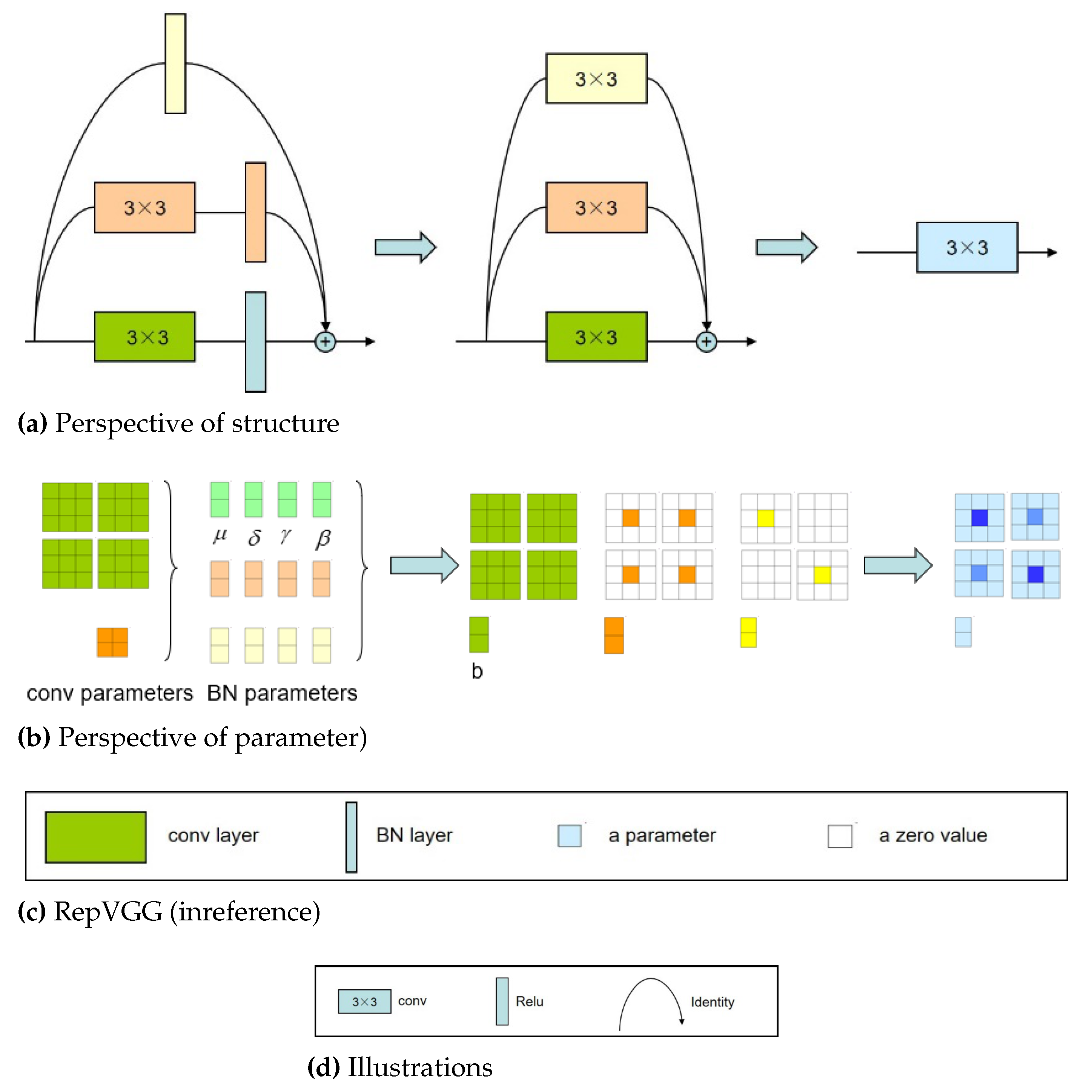
To improve the performance of deep learning without making the network structure increasingly more and more complex, Ding et al. [38] proposed RepVGG algorithm, a VGG-style architecture which outperforms many complicated models. The VGG-style architecture has the following characteristics: (1) The architecture has no branch structure; (2) The architecture only applies convolution; (3) The architecture only uses ReLU as the activation function. The sketch of RepVGG architecture is shown in Figure 6. The RepVGG architecture was inspired by ResNet so it also uses identity and branches, but only for training. After training, the trained RepVGG model needs to be transformed equivalently to get the deployment model. A convolution can be considered as a special convolution with many zeros in a special convolution kernel, while a constant mapping is a special convolution with a unit matrix as the convolution kernel. Therefore, according to the additivity of convolution, the three branches of each RepVGG block can be combined into a convolution.
Figure 6 describes the convolution conversion method of RepVGG. In [38], the input and output channels are both 2, so the parameter of convolution is four matrices, and the parameter of convolution is a matrix. Please note that each of the three branches has a batch normalization (BN) layer, and its parameters include the accumulated mean and standard deviation, the learned scaling factor and bias. After transforming the convolution layer and BN layer of the three branches into a convolution layer with bias, the convolution kernel is transformed into by 0 for padding. In this way, the output of each RepVGG block before and after conversion is exactly the same, so the trained model can be converted to a single channel model with only convolution.
Next, we describe how to transform a training block into a separate convolutional layer for reasoning as shown in Figure 7. Formally, was used to express the kernel of convolutional layer with input channel and output channel. was used to express the kernel of branch layer. was used to express the mean value, standard deviation, learning factor and deviation of BN layer respectively after convolutional layer. In addition, was identity branch. We set , as input and output respectively, * as convolution operator. If , , , then we can get Equation (1).
Otherwise, if identity branch is not used, Equation (1) has only the first two terms. Here BN is the inference time BN function. Formally, we can get Equation (2).
Each BN and its preceding convolution layer are converted into a convolution with a bias vector. Then, let be the kernel and bias converted from Then we can get Equations (3) and (4).
Then it is easy for us to verity that we can get Equation (5)
The above transformation is also applicable to identity branch, for identity mapping can be regarded as convolution with identity matrix as the kernel.
4.2. Introduction of Spatial Attention Mechanism
Attention can be understood as weighted summation, i.e., for weights that are originally distributed equally, they are redistributed according to the importance of the object of attention. The important units are given more points, and the unimportant or bad units are given less points. Wang et al. [39] first proposed non local operations, which use self attention mechanism to establish remote dependence. This is the first application of attention mechanism in computer vision. Attention mechanism can be divided into many kinds: spatial attention mechanism, channel attention mechanism, mixed attention mechanism etc. The attention mechanism used in this paper is spatial attention mechanism, which can be seen in [40].The spatial attention module is shown in Figure 8.
According to [40], max pooling and average pooling are used in channel dimension to get two different feature descriptions and . Then, concatenation is used to merge the two feature descriptions, and convolution is used to generate spatial attention map . In short, the spatial attention is computed as Equation (6).
where enotes the sigmoid function and represents a convolution operation with the filter size of .
4.3. Introduction of Spatial Attention Mechanism
Considering the excellent performance of RepVGG algorithm in ImageNet dataset, we decided to apply it to steel strip defect classification. Since adding attention mechanism can improve the classification accuracy of deep learning algorithm, we decided to combine spatial attention mechanism with RepVGG algorithm. We argue that the performance of RepVGG network with spatial attention mechanism will be greatly improved than that of the original network. In the next part of this article, we will design experiments to prove our conjecture and compare it with many other networks. The version of RepVgg we chose is RepVgg_B3g4, more details about the algorithm can be found at https://github.com/Fighter20092392/X-SDD-A-New-benchmark (accessed on 18 January 2021).
5. Experiments
5.1. Experimental Environment
The experimental environment is equipped with a single NVIDIA RTX2080S GPU, an Intel Core i7-9700 CPU, a 16GB of RAM, Windows 10 operating system and PyTorch deep learning framework. In the experiment, the image size is adjusted to pixels, the mini-batch of model training is 10, the whole training is 100 epochs, the learning rate is set to 0.0001, and the Adam optimization algorithm is used to optimize the model.
We use 70% of the data in X-SDD as the trainset and 30% of the data in X-SDD as the testset. Therefore, the trainset contains 952 images while the testset contains 408 images. Our experiments were conducted on the anaconda platform.
5.2. Experimental Results
To make the experimental results more convincing, we compared several metrics, including Accuary, Macro-recall, Macro-precision, and Macro-F1. Macro-Recall, Macro-precision, and Macro-F1 are obtained by averaging the Recall, Precision, F1-score of each category after considering the multiclassification problem as multiple binary classification problems. Recall, Precision and F1 in the binary classification problem are given by Equations (7)–(9).
where denotes true positive, which is the number of positive samples classified correctly. denotes true negative, which is the number of negative samples classified correctly. denotes false postive, which is the number of negative samples classified as postive. denotes false negative, which is the number of postive samples classified as negative. aking each class of the multiclassification separately and combining the other classes as one class, we can find , , , of each class separately. Based on the above indicators for each category, we can obtain Equations (10)–(14).
where is the number of categories, is the total number of samples, and are abbreviations of Precision and Recall respectively.
The experimental results are shown in Table 1. It can be seen from Table 1 that multiple deep learning algorithms have achieved 87.01–95.10% Accuracy, 82.04–93.92% Macro-Recall, 82.04–95.16% Macro-Precision, 81.58–93.25% Macro-F1 on X-SDD we proposed. The above facts show that there are differences in the results of different deep learning models tested on X-SDD, and our X-SDD can provide a data resource for the research of deep learning algorithms.
In addition, according to [41], ResNet50 achieves better results in the field of strip steel classification compared to other models. In this paper, the model achieves results second only to our proposed RegVGG+SA model in both Accuary and Macro-Precision metrics. In addition, on both Macro-Recall and Macro-F1 metrics, the ResNet50 model achieved the third best performance. Our test results demonstrate the effectiveness of the ResNet50 model used in [41], while our proposed RepVGG+SA model is more advantageous with respect to the ResNet50 model. Compared with other models, our proposed RepVGG+SA model achieves the best performance in all of the four metrics: Accuary, Macro-Recall, Macro-Precision and Macro-F1. The experimental results show that the algorithm we proposed is effective in the field of hot strip defect classification. Moreover, The classification accuracy of more than 95% proves that the algorithm proposed in this paper has enough engineering practical value, and can be used in the actual strip defect classification. The 93.92% of Macro-Recall, 95.16% of Macro-Precision and 93.25% of Macro-F1 proves that our RepVGG+SA has some advantageous in handling unbalanced hot rolled steel strip defects images.
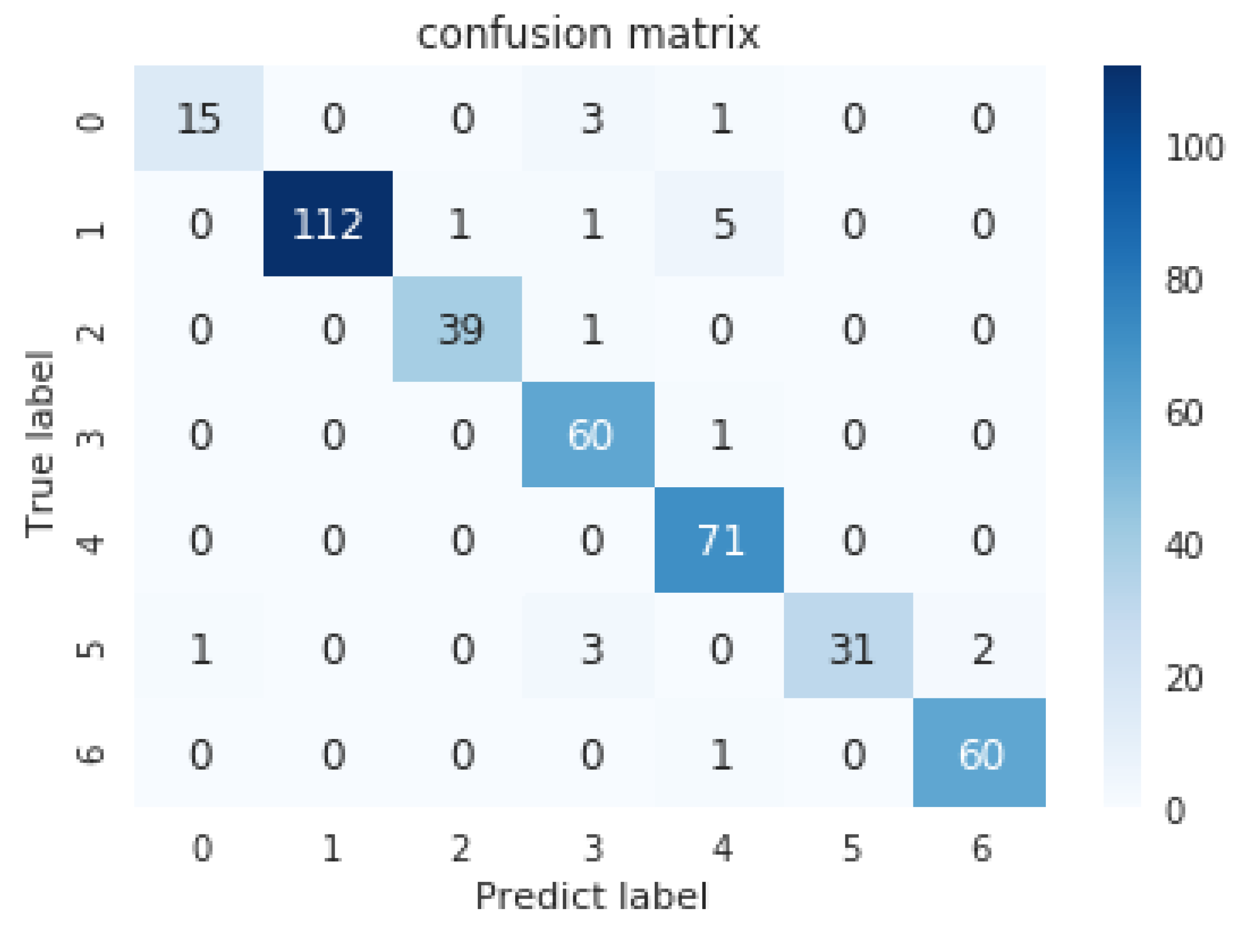
The confusion matrix of RepVGG+SA algorithm is shown in Figure 9. It can be seen from the figure that our proposed RepVGG+SA algorithm has high classification accuracy for each category in the dataset. Among them, the algorithm has the highest accuracy in classifying the defects of finishing roll printing, reaching 100%. One possible reason for the algorithm’s 100% accuracy in classifying this type of defect is that the characteristic morphology of the finishing roll printing defect is more pronounced and differs significantly from the characteristics of other defects. To see more intuitively the classification accuracy of our proposed algorithm on each defect category, we display it in the form of a table, as shown in Table 2.
It can be seen from Table 2 that the classification accuracy of our model is low, and the classification accuracy is 78.95%. There are two reasons for the low classification accuracy of this category: one is that the sample size of this category is relatively small, and the model does not learn enough about the characteristics of this category; the other is that the morphology of plate channel scale and slag inclusion is relatively close, which is prone to misclassification, which leads to several plate channel scale being classified as slag inclusion in the testset. Using cascade structure or integrating multiple different algorithms may help to solve the problem of low classification accuracy. Next we analyze the model complexity and the relevant results are shown in Table 3.
It can be seen from Table 3 that our proposed RegVGG+SA model is relatively large in terms of both number of parameters and computational complexity. Compared to the lightweight deep learning model EspNet-v2 with 0.627 M and 0.090 G in the number of parameters and computational complexity, respectively, our proposed model has 83.825 M and 17.892 G in these two metrics, respectively. This indicates that our proposed RepVGG+SA model is more costly in terms of computational complexity while achieving good classification accuracy. In the future study, we will try to reduce the computational complexity of the model in order to reduce its deployment cost.
6. Discussion and Conclusions
In the research field of hot rolled steel strip surface defect detection, the surface defect datasets are crucial, and although there are commonly used NEU-CLS datasets, they are still not sufficient to completely solve the problem of lack of steel strip surface defect datasets. To make some contribution to solve the limitation of defect dataset on the research of defect classification, a defect data set of hot rolled steel strip is proposed in this paper. The dataset, named Xsteel surface defect dataset (X-SDD), contains seven kinds of 1360 defect images from the hot steel strip rolling site. Compared with the existing NEU-CLS, our dataset has one more categories.Meanwhile, there is a big difference between X-SDD and NEU-CLS. This shows that our dataset can be used as an important supplement to NEU-CLS, thus researchers can verify the algorithm on X-SDD and NEU-CLS respectively. On this basis, due to the imbalance of the number of samples in X-SDD, it provides conditions for researchers to solve the problem of sample imbalance.
In this paper, we apply a variety of algorithms to verify the effectiveness of our proposed X-SDD, and introduce the recently proposed RepVGG algorithm to combine it with spatial attention mechanism.The comparison results show that ResNet50, used in the literature [41], achieves results on Accuracy and Macro-Precision that are second only to our proposed RepVGG+SA algorithm. As for Macro-Recall and Macro-F1, ResNet50 achieved the third best result. The excellent performance of ResNet50 in strip classification indicates that the residual network has some advantages in the classification of strip defects. In addition, ResNet50 performs better on X-SDD than the deeper ResNet101 and 152, indicating that the deeper the network level is not better when the amount of data is not particularly large. In addition, our RepVGG+SA algorithm achieves promising results, while the metrics of Accuracy, Macro-Recall, Macro-Precision, Macro-F1 are all the best among numerous algorithms. The classification accuracy of RepVGG+SA algorithm is 95.10% on this dataset, while the classification accuracy of single memory RepVGG algorithm is 91.67%, which indicates that the mechanism of adding spatial attention is effective and the RepVGG+SA algorithm has some advantages in dealing with the imbalanced sample problem.
Although the experimental results prove the effectiveness of the RepVGG+SA algorithm, we can observe that on a relatively small number of defects such as oxide scale of plate system, the performance of the algorithm is not very well, with a classification accuracy of only 78.95%. To solve the problem of low accuracy in individual category classification, we argue that when the sample size is more sufficient or cascade structure is adopted, the classification accuracy will be improved. In addition, if artificial prior knowledge can be added to deep learning, e.g., combining manual feature extraction with deep learning feature extraction methods, it may help to improve the classification accuracy when the sample is not very sufficient.
In the future, we may continue to study from the following two aspects: one is to collect and update the existing sample library. We argue that more high-quality samples from the scene will help researchers to propose better performance algorithms. The other is that we will consider using the improved transformer [42] algorithm to classify the surface defects of steel strip. The improved version of the transformer was proved to have excellent performance in the field of classification. We believe that it can provide a new idea for the classification of steel strip defects. Our further research plan for the algorithm is as follows: Firstly, considering the excellent performance of the VIT [43] algorithm on the classification problem, we plan to apply the algorithm to strip surface defects classification. Secondly, considering that the VIT algorithm is not satisfactory for classification with small datasets, we will explore to improve the structure of this algorithm or and use suitable data augmentation, so that the improved VIT algorithm has excellent. Last but not least, the original VIT algorithm is not conducive to practical applications in engineering due to its large time overhead in the inference process; therefore, we will investigate ways to speed up its inference efficiency in conjunction with the latest references.
Author Contributions
Conceptualization, X.F. and L.L.; methodology, X.F.; software, X.F.; validation, X.F. and L.L.; formal analysis, X.G.; investigation, X.F.; resources, X.G.; data curation, X.F.; writing—original draft preparation, X.F.; writing—review and editing, L.L.; visualization, X.G.; supervision, X.G.; project administration, X.G.; funding acquisition, X.G. All authors have read and agreed to the published version of the manuscript.
Funding
This research was funded by National Science Foundation under Grant 61573087 and 61573088.
Data Availability Statement
The dataset is available at: https://github.com/Fighter20092392/X-SDD-A-New-benchmark (accessed on 18 March 2021).
Acknowledgments
This work is done when X.F. was an intern at xBang Inc., Shenyang, China. Thanks their support for this work.
Conflicts of Interest
The authors declare no conflict of interest.
References
- Aldunin, A. Development of method for calculation of structure parameters of hot-rolled steel strip for sheet stamping. J. Chem. Technol. Metall. 2017, 52, 737–740. [Google Scholar]
- Xu, Z.; Liu, X.; Zhang, K. Mechanical Properties Prediction for Hot Rolled Alloy Steel Using Convolutional Neural Network. IEEE Access 2019, 7, 47068–47078. [Google Scholar] [CrossRef]
- Kumar, A.; Das, A.K. Evolution of microstructure and mechanical properties of Co-SiC tungsten inert gas cladded coating on 304 stainless steel. Eng. Sci. Technol. Int. J. 2020, 24, 591–604. [Google Scholar]
- Afanasieva, L.E.; Ratkevich, G.V.; Ivanova, A.I.; Novoselova, M.V.; Zorenko, D.A. On the Surface Micromorphology and Structure of Stainless Steel Obtained via Selective Laser Melting. J. Surf. Investig. X-Ray Synchrotron Neutron Tech. 2018, 12, 1082–1087. [Google Scholar] [CrossRef]
- Gromov, V.E.; Gorbunov, S.V.; Ivanov, Y.F.; Vorobiev, S.V.; Konovalov, S.V. Formation of surface gradient structural-phase states under electron-beam treatment of stainless steel. J. Surf. Investigation. X-Ray Synchrotron Neutron Tech. 2011, 5, 974–978. [Google Scholar] [CrossRef]
- Luo, Q.; Fang, X.; Sun, Y.; Liu, L.; Ai, J.; Yang, C.; Simpson, O. Surface Defect Classification for Hot-Rolled Steel Strips by Selectively Dominant Local Binary Patterns. IEEE Access 2019, 7, 23488–23499. [Google Scholar] [CrossRef]
- Ashour, M.W.; Khalid, F.; Halin, A.A.; Abdullah, L.N.; Darwish, S.H. Surface defects classification of hot-rolled steel strips using multi-directional shearlet features. Arab. J. Sci. Eng. 2019, 44, 2925–2932. [Google Scholar] [CrossRef]
- Youkachen, S.; Ruchanurucks, M.; Phatrapomnant, T.; Kaneko, H. Defect Segmentation of Hot-rolled Steel Strip Surface by using Convolutional Auto-Encoder and Conventional Image processing. In Proceedings of the 2019 10th International Conference of Information and Communication Technology for Embedded Systems (IC-ICTES), Bangkok, Thailand, 25–27 March 2019; pp. 1–5. [Google Scholar] [CrossRef]
- Kostenetskiy, P.; Alkapov, R.; Vetoshkin, N.; Chulkevich, R.; Napolskikh, I.; Poponin, O. Real-time system for automatic cold strip surface defect detection. FME Trans. 2019, 47, 765–774. [Google Scholar] [CrossRef] [Green Version]
- Mazur, I.; Koinov, T. Quality Control system for a hot-rolled metal surface. Frat. Ed Integrità Strutt. 2016, 10, 287–296. [Google Scholar] [CrossRef] [Green Version]
- Severstal is Mastering the Production of Video Inspection Systems for Rolled Surfaces. Available online: https://metallurgprom.org/en/press-releases/4952-severstal-osvaivaet-izgotovlenie-sistem-videoinspekcii-poverhnosti-prokata.html (accessed on 18 January 2021).
- Kim, C.H.; Choi, S.H.; Kim, G.B.; Joo, W.J. Classification of surface defect on steel strip by KNN classifier. J. Korean Soc. Precis. Eng. 2006, 23, 80–88. [Google Scholar]
- Karthikeyan, S.; Pravin, M.C.; Sathyabama, B.; Mareeswari, M. DWT Based LCP Features for the Classification of Steel Surface Defects in SEM Images with KNN Classifier. Aust. J. Basic Appl. Sci. 2016, 10. Available online: https://ssrn.com/abstract=2792637 (accessed on 17 April 2021).
- Zaghdoudi, R.; Seridi, H.; Boudiaf, A. Multiple classifier combination for steel surface inspection. In Proceedings of the 2nd Conference on Informatics and Applied Mathematics, IAM 2019, Guelma, Algeria, 24–25 April 2019. [Google Scholar]
- Peng, K.; Zhang, X. Classification technology for automatic surface defects detection of steel strip based on improved BP algorithm. In Proceedings of the Fifth International Conference on Natural Computation, Tianjian, China, 14–16 August 2009; pp. 110–114. [Google Scholar]
- Amid, E.; Aghdam, S.R.; Amindavar, H. Enhanced performance for support vector machines as multi-class classifiers in steel surface defects detection. World Acad. Sci. Eng. Technol. 2012, 6, 1096–1100. [Google Scholar]
- Schleif, F.M.; Tino, P. Indefinite core vector machine. Pattern Recogn. 2017, 71, 187–195. [Google Scholar] [CrossRef] [Green Version]
- Xiao, M.; Jiang, M.; Li, G.; Xie, L.; Yi, L. An evolutionary classifier for steel surface defects with small sample set. EURASIP J. Image Video Process. 2017, 2017, 48. [Google Scholar] [CrossRef] [Green Version]
- Gong, R.; Wu, C.; Chu, M. Steel surface defect classification using multiple hyper-spheres support vector machine with additional information. Chemom. Intell. Lab. Syst. 2018, 172, 109–117. [Google Scholar] [CrossRef]
- Peng, X.; Xu, D. Twin support vector hypersphere (TSVH) classifier for pattern recognition. Neural Comput. Appl. 2014, 24, 1207–1220. [Google Scholar] [CrossRef]
- Cevikalp, H. Best fitting hyperplanes for classification. IEEE Trans. Pattern Anal. Mach. Intell. 2017, 39, 1076–1088. [Google Scholar] [CrossRef]
- Liu, Y.; Xu, K.; Xu, J. An improved MB-LBP defect recognition approach for the surface of steel plates. Appl. Sci. 2019, 9, 4222. [Google Scholar] [CrossRef] [Green Version]
- Krizhevsky, A.; Sutskever, I.; Hinton, G.E. ImageNet classi-fication with deep convolutional neural networks. In Proceedings of the 25th International Conference on Neural Information Processing Systems, Lake Tahoe, NV, USA, 3–6 December 2012; Curran Associates Inc.: Lake Tahoe, NV, USA, 2012; pp. 1097–1105. [Google Scholar]
- Simonyan, K.; Zisserman, A. Very deep convolutional networks for large-scale image recognition. arXiv 2014, arXiv:1409.1556. [Google Scholar]
- Szegedy, C.; Liu, W.; Jia, Y.; Sermanet, P.; Reed, S.; Anguelov, D.; Erhan, D.; Vanhoucke, V.; Rabinovich, A. Going deeper with convolutions. In Proceedings of the 2015 IEEE Conference on Computer Vision and Pattern Recognition, Boston, MA, USA, 7–12 June 2015; pp. 1–9. [Google Scholar]
- He, K.M.; Zhang, X.Y.; Ren, S.Q.; Sun, J. Deep residual learning for image recognition. In Proceedings of the 2016 IEEE Conference on Computer Vision and Pattern Recognition, LasVegas, NV, USA, 27–30 June2016; pp. 770–778. [Google Scholar]
- Huang, G.; Liu, Z.; Van, D.M.L.; Weinberger, K.Q. Densely connected convolutional networks. In Proceedings of the 2017 IEEE Conference on Computer Vision and Pattern Recognition, Honolulu, HI, USA, 21–26 July 2017; pp. 4700–4708. [Google Scholar]
- Hu, J.; Shen, L.; Sun, G. Squeeze-and-excitation networks. In Proceedings of the 2018 IEEE/CVF Conference on Computer Vision and Pattern Recognition, Salt Lake City, UT, USA, 18–23 June 2018; pp. 7132–7141. [Google Scholar]
- Zhang, X.Y.; Zhou, X.Y.; Lin, M.X.; Sun, J. Shufflenet: An extremely efficient convolutional neural network for mobile devices. In Proceedings of the 2018 IEEE/CVF Conference onComputer Vision and Pattern Recognition, Salt Lake City, UT, USA, 18–23 June 2018; pp. 6848–6856. [Google Scholar]
- Howard, A.G.; Zhu, M.; Chen, B.; Kalenichenko, D.; Wang, W.; Wey, T.; Andreetto, M.; Adam, H. Mobilenets: Efficient convolutional neural networks for mobile vision applications. arXiv 2017, arXiv:1704.04861. [Google Scholar]
- Song, K.; Yan, Y. Micro Surface defect detection method for silicon steel strip based on saliency convex active contour model. Math. Probl. Eng. 2013, 2013, 429094. [Google Scholar] [CrossRef]
- Dong, H.; Song, K.; He, Y.; Xu, J.; Yan, Y.; Meng, Q. PGA-Net: Pyramid Feature Fusion and Global Context Attention Network for Automated Surface Defect Detection. IEEE Trans. Ind. Inf. 2020, 16, 7448–7458. [Google Scholar] [CrossRef]
- He, Y.; Song, K.; Meng, Q.; Yan, Y. An End-to-end Steel Surface Defect Detection Approach via Fusing Multiple Hierarchical Features. IEEE Trans. Instrum. Meas. 2020, 69, 1493–1504. [Google Scholar] [CrossRef]
- Zhang, D.; Song, K.; Xu, J.; He, Y.; Yan, Y. Unified Detection Method of Aluminium Profile Surface Defects: Common and Rare Defect Categories. Opt. Lasers Eng. 2020, 126, 105936. [Google Scholar] [CrossRef]
- Gao, Y.; Gao, L.; Li, X.; Yan, X. A semi-supervised convolutional neural network-based method for steel surface defect recognition. Robot. Comput. Integr. Manuf. 2020, 61, 101825. [Google Scholar] [CrossRef]
- Luo, Q.; Fang, X.; Liu, L.; Yang, C.; Sun, Y. Automated Visual Defect Detection for Flat Steel Surface: A Survey. IEEE Trans. Instrum. Meas. 2020, 69, 626–644. [Google Scholar] [CrossRef] [Green Version]
- Zhang, Z. Analysis the Causes of Scale on Hot Rolled Strips & Its Prevention Measures; Xinjiang Bayi Iron & Steel Stock Co., Ltd.: Ürümqi, China, 2009; pp. 41–44. [Google Scholar]
- Ding, X.; Zhang, X.; Ma, N.; Han, J.; Ding, G.; Sun, J. RepVGG: Making VGG-style ConvNets Great Again. arXiv 2021, arXiv:2101.03697. [Google Scholar]
- Wang, X.; Girshick, R.; Gupta, A.; He, K. Non-local neural networks. In Proceedings of the IEEE Conference on Computer Vision and Pattern Recognition 2018, Salt Lake City, UT, USA, 18–22 June 2018; pp. 7794–7803. [Google Scholar]
- Woo, S.; Park, J.; Lee, J.Y.; Kweon, I.S. Cbam: Convolutional block attention module. In Proceedings of the European Conference on Computer Vision (ECCV) 2018, Salt Lake City, UT, USA, 18–22 June 2018; pp. 3–19. [Google Scholar]
- Konovalenko, I.; Maruschak, P.; Brezinová, J.; Viňáš, J.; Brezina, J. Steel Surface Defect Classification Using Deep Residual Neural Network. Metals 2020, 10, 846. [Google Scholar] [CrossRef]
- Vaswani, A.; Shazeer, N.; Parmar, N.; Uszkoreit, J.; Jones, L.; Gomez, A.N.; Kaiser, L.; Polosukhin, I. Attention is all you need. arXiv 2017, arXiv:1706.03762. [Google Scholar]
- Dosovitskiy, A.; Beyer, L.; Kolesnikov, A.; Weissenborn, D.; Zhai, X.; Unterthiner, T.; Dehghani, M.; Minderer, M.; Heigold, G.; Gelly, S.; et al. An image is worth 16x16 words: Transformers for image recognition at scale. arXiv 2020, arXiv:2010.11929. [Google Scholar]
Figure 1.
Coils of steel strip.

Figure 2.
Machine vision defect detection system.

Figure 3.
Samples of seven kinds of typical surface on X-SDD. ((a)—inclusion, (b)—red iron sheet, (c)—iron sheet ash, (d)—scratches, (e)—oxide scale of plate system, (f)—finishing roll printing and (g)—oxide scale of temperature system).
Figure 3.
Samples of seven kinds of typical surface on X-SDD. ((a)—inclusion, (b)—red iron sheet, (c)—iron sheet ash, (d)—scratches, (e)—oxide scale of plate system, (f)—finishing roll printing and (g)—oxide scale of temperature system).

Figure 4.
Samples of six kinds of typical surface on NEU-CLS. ((a)—crazing, (b)—inclusion, (c)—patches, (d)—pitted surface, (e)—rolled in scale, (f)—scrathes).
Figure 4.
Samples of six kinds of typical surface on NEU-CLS. ((a)—crazing, (b)—inclusion, (c)—patches, (d)—pitted surface, (e)—rolled in scale, (f)—scrathes).

Figure 5.
The number of defects.

Figure 6.
The Sketch of RepVGG architecture.

Figure 7.
Structural re-parameterization of a RepVGG block.

Figure 8.
The spatial attention module.

Figure 9.
The confusion matrix.


Table 1.
The experimental results.
| Model | Accuary | Macro-Recall | Macro-Precision | Macro-F1 |
|---|---|---|---|---|
| EspNet-v2 | 89.95% | 84.19% | 88.28% | 84.28% |
| GhostNet | 88.72% | 87.87% | 86.93% | 87.07% |
| ShuffleNet | 87.50% | 85.84% | 84.83% | 84.68% |
| SqueezeNet | 91.42% | 83.21% | 90.36% | 84.15% |
| Xception | 90.44% | 87.39% | 89.41% | 88.25% |
| VGG16 | 92.65% | 90.46% | 91.70% | 90.92% |
| ResNet50 | 93.87% | 89.41% | 93.45% | 90.02% |
| ResNet101 | 87.01% | 88.30% | 88.18% | 87.05% |
| ResNet152 | 92.16% | 89.41% | 91.41% | 89.92% |
| RepVGG_B1g2 | 88.97% | 82.04% | 90.79% | 81.58% |
| RepVGG_B3g4 | 91.67% | 85.28% | 88.46% | 84.94% |
| RepVGG_B3g4+SA(ours) | 95.10% | 93.92% | 95.16% | 93.25% |
Table 2.
The Classification results of RepVGG+SA.
| Defect Category/Indicators | Right | Error | Total Number | Accuary |
|---|---|---|---|---|
| oxide scale of plate system | 15 | 4 | 19 | 78.95% |
| red iron sheet | 112 | 7 | 119 | 94.12% |
| scratches | 39 | 1 | 40 | 97.50% |
| inclusion | 60 | 1 | 61 | 98.36% |
| finishing roll printing | 71 | 0 | 71 | 100% |
| iron sheet ash | 31 | 6 | 37 | 83.78% |
| oxide scale of temperature system | 60 | 1 | 61 | 98.36% |
| total | 388 | 20 | 408 | 95.10% |
Table 3.
The Comparison of Model Parameters and Complexity.
| Model | Params (M) | MACs (G) |
|---|---|---|
| EspNet-v2 | 0.627 | 0.090 |
| GhostNet | 3.127 | 0.208 |
| ShuffleNet | 0.840 | 0.129 |
| SqueezeNet | 0.722 | 0.720 |
| Xception | 20.822 | 4.617 |
| VGG16 | 134.289 | 15.480 |
| ResNet50 | 23.522 | 4.109 |
| ResNet101 | 42.515 | 7.832 |
| ResNet152 | 58.158 | 11.557 |
| RepVGG_B1g2 | 43.748 | 9.815 |
| RepVGG_B3g4 | 81.282 | 17.888 |
| RepVGG_B3g4+SA(ours) | 83.825 | 17.892 |
Publisher’s Note: MDPI stays neutral with regard to jurisdictional claims in published maps and institutional affiliations. |
© 2021 by the authors. Licensee MDPI, Basel, Switzerland. This article is an open access article distributed under the terms and conditions of the Creative Commons Attribution (CC BY) license (https://creativecommons.org/licenses/by/4.0/).
Share and Cite
MDPI and ACS Style
Feng, X.; Gao, X.; Luo, L. X-SDD: A New Benchmark for Hot Rolled Steel Strip Surface Defects Detection. Symmetry 2021, 13, 706. https://doi.org/10.3390/sym13040706
AMA Style
Feng X, Gao X, Luo L. X-SDD: A New Benchmark for Hot Rolled Steel Strip Surface Defects Detection. Symmetry. 2021; 13(4):706. https://doi.org/10.3390/sym13040706
Chicago/Turabian StyleFeng, Xinglong, Xianwen Gao, and Ling Luo. 2021. "X-SDD: A New Benchmark for Hot Rolled Steel Strip Surface Defects Detection" Symmetry 13, no. 4: 706. https://doi.org/10.3390/sym13040706
Note that from the first issue of 2016, this journal uses article numbers instead of page numbers. See further details here.