
Stochastic Analysis of Train Running Safety on Bridge with Earthquake-Induced Irregularity under Aftershock

1
School of Civil Engineering, Central South University, Changsha 410075, China
2
Department of Building Engineering, University of Huanghuai, No. 6 Kaiyuan Road, Zhumadian 463000, China
*
Author to whom correspondence should be addressed.
Symmetry 2022, 14(10), 1998; https://doi.org/10.3390/sym14101998
Submission received: 29 July 2022
/
Revised: 13 September 2022
/
Accepted: 18 September 2022
/
Published: 23 September 2022
(This article belongs to the Special Issue Symmetry in Applied Mechanics Analysis on Smart Optical Fiber Sensors)
Abstract
:As a type of urban life project in China, bridges need a certain capacity of trains running safely after an earthquake to ensure and guarantee transportation on railway lines, post-disaster reconstruction and relief work. Since aftershocks may occur after the main shock, the earthquake-induced irregularity and aftershock intensity are fully considered, based on the running safety index in the seismic design of bridges. However, there is a lack of research on the running safety of trains after an earthquake; it is mainly judged on experience, and lacks theoretical basis. In this paper, the established finite element model of a train bridge interaction system with symmetry was considered. The point estimation method (PEM) combined with moment expansion approximation (MEA) is used for random calculation of the Housner Intensity (HI). Furthermore, running safety indexes were analyzed and the running safety performance of a simply supported bridge with symmetry was assessed under a post-earthquake condition. Then the limit value, to ensure the traffic safety performance after an earthquake, is calculated based on stochastic analysis. The HI can be calculated with full consideration of the randomness of aftershock intensity and structural parameters. On this basis, a calculation method of the HI that considers the randomness of aftershock intensity is proposed. This study can be helpful for the performance-based design of symmetric railway structures under post-earthquake conditions.
1. Introduction
The urban life project refers to the key department that directly maintains the normal operation of a city, and reduces emergencies under disaster conditions. It is related to the survival of the city. As an important part of the urban life project, bridges are the main projects of urban traffic lines; however, there is a lack of research on the running safety of trains after earthquakes. It is mainly judged on experience due to the lack of pertinent theory. In addition, people are not only concerned about damage and collapse caused by disasters (such as an earthquake), but also secondary disasters (indirect economic losses caused by traffic interruption and destruction of other facilities, even threatening people’s life safety in serious cases), which are very serious. Relevant experts all over the world have proposed a three-stage seismic design method for bridge structures based on these three levels: they do not get damaged in a small earthquake, they are repairable in a medium earthquake, and they do not collapse in a large earthquake”.
The technical measures for disaster prevention and mitigation of urban bridges mainly include [1]: (1) Disaster monitoring: including disaster precursor monitoring, disaster development trend monitoring, etc. (2) Disaster prediction: including the prediction of potential disasters and their occurrence time, scope and scale, so as to prepare for effective disaster prevention. (3) Disaster prevention: taking preventive measures against natural disasters, which are the least costly and effective disaster reduction measures. (4) Disaster resistance: engineering measures taken against disasters. (5) Disaster relief: the most urgent disaster reduction measure once the disaster has started.
In order to maintain the urban life project and designate relief work effective, the traffic performance of bridges after an earthquake is the key ingredient of the whole process [2,3]. Based on this consideration, some scholars have undertaken research on rail deformation and traffic safety after an earthquake [4,5,6,7,8]. Liu and Lai use the staggered station to determine whether trains are allowed to pass at a slow speed, so as to ensure the transportation of supplies and rescue workers to a certain extent [6,7], but most of them are based on using the train response to analyse the running safety. At present, there is a lack of research on the project that determines whether trains are allowed to pass over the bridge by analyzing the bridge response. Moreover, as a typical secondary disaster, the aftershock excitation effect has sufficient probability to happen when driving after main earthquake. In addition, according to Yu’s studies, earthquake-induced rail deformation is a complex random process [8,9]; it is too simple to estimate it only by using the staggered station. Furthermore, the earthquake-induced rail irregularity is closely related to the dynamic characteristics of earthquake and bridge. Additionally, Yu et al. [9] proposed that the spectrum of the earthquake-induced irregularity can be fitted with a mathematical formula; this provides the possibility of random analysis of earthquake-induced rail deformation.
As for the running safety assessment of trains in the seismic design of railway structures, Luo et al. proposed a set of calculation methods for the driving safety performance of bridges under earthquake excitation [10,11]. However, Luo did not consider earthquake-induced rail deformation, but the method provides a theoretical basis for traffic safety after earthquake analysis that considers aftershocks. Based on this, the traffic performance of a bridge after an earthquake is studied in this paper.
In addition, the intensity of the aftershock is a typical random variable. It is worth noting that aftershock intensity is not considered to be a Gaussian random process [12,13] poses a problem in the upper limit calculation of the confidence interval for stochastic analysis. In this regard, Mao et al. studied a stochastic dynamic model of a train–track–bridge coupled system based on the probability density evolution method [14,15,16], and Liu et al. proposed a stochastic analysis method [17,18,19,20,21] based on the Karhunen–Loeve expansion and point estimate method, which can be used to efficiently and accurately calculate the random response of a Train–Bridge Interaction System (TBIS) with multiple random factors. Xu and Yu et al. [15,22,23] studied vehicle–track random vibrations considering spatial frequency coherence of track irregularities, but most of the random variables they studied were Gaussian random variables, which means the confidence intervals for response results can be simply calculated by the three-sigma rule [24,25,26]. At present, few stochastic analysis methods have been successfully applied to non-Gaussian vehicle–bridge systems. When considering the non-Gaussian variables, confidence intervals cannot be calculated simply on the basis of a three-sigma rule. Thus in this paper, the moment expansion approximation (MEA) [27] is used to stochastically analyze the upper limit of running safety indexes.
Therefore, according to the above content, the train running safety on a bridge with earthquake-induced irregularity under an aftershock was studied, which has not been fully studied by other scholars. This was in order to provide a design basis for determining whether the train can pass over the bridge or not via the response of bridge. Based on the post-earthquake condition, this paper considered the randomness of earthquake-induced irregularity and the randomness of the intensity of the aftershocks, and established the finite element model of the TBIS to calculate the safety limit of the indexes of the running safety of the bridge. It is instructive to the safety performance and structural health monitoring of bridge traffic of post-earthquake [28,29].
2. Methodology
The overall process of the work in this paper is listed in Figure 1:
2.1. Earthquake-Induced Irregularity Generated by the Karhunen-Loeve Expansion (KLE) and the Trigonometric Series Method (TSM)
Yu and Lai undertook much research [4,8,9,30] on the spectrum representation of earthquake-induced rail deformation through the ANSYS modeling and shaking table experiment [31]. They inputted a large number of earthquake samples, and proposed a simply supported bridge earthquake-induced irregularity spectrum by combining hypothesis testing with Fourier transform for the study of the running safety of trains after earthquakes. At present, it is increasingly important to focus on track irregularities caused by earthquakes. The study is the basis for ensuring traffic safety after the occurrence of earthquakes. The results show that the earthquake-induced irregularity can be generated by the irregularity spectrum, and it is a typical stationary zero-mean Gaussian stochastic process.
According to Yu’s research, random characteristics of earthquake-induced rail irregularities can be expressed by a spectrum formula. This section uses two methods to generate random irregularity samples, and it verifies the accuracy and reliability of the method applied to post-earthquake disobedience.
In basic terms, the trigonometric series method (TSM) is a common approach in generating a random process from a type of spectrum, which can be written as:
where and .
Meanwhile the Karhunen–Loeve Expansion represents random processes by using a set of random variables and deterministic eigenfunctions and eigenvalues.
and are the eigenvalues and eigenfunctions of the covariance matrix of the random process, is a set of uncorrelated standard Gaussian random variables, and is the mean value of the stochastic process. More details of the KLE can be found in [18]; M is set to 300 for accuracy of the KLE in this section.
In this paper, the KLE and the TSM were used to generate samples of earthquake-induced irregularity, as shown in Figure 2a. By extracting the power spectrum of them, as shown in Figure 2b,d, it is found that both methods have good accuracy. In addition, there is a further point to note. According to the KS test analysis, the earthquake-induced rail irregularity is a Gaussian random process, as shown in Figure 2c.
2.2. PEM for Stochastic Analysis
According to the studies, HI only depends on bridge response and earthquake-induced irregularity is irrelevant. In addition, although the aftershock intensity is small, it can also significantly affect the response of the bridge. The aftershock intensity is a relatively random parameter.
In this paper, the Gutenberg–Richter (G–R) distribution is used to predict aftershocks, which suggests that strong earthquakes are less likely to occur, and weaker earthquakes have a higher probability of occurring.
where , represents the magnitude, and and are the lower and upper limits of seismic magnitude. In this paper, to predict the likelihood of aftershock magnitude, is set as 4.0, and it is empirically shown that the difference between the mainshock magnitude and its largest aftershock magnitude is about 1.2 magnitudes less than the mainshock magnitude; As a result, is set as subtracting 1.2 from the main earthquake magnitude [13].
The attenuation relation of ground motion is adopted as
where A, B, C, D, E are 3.706, 0.298, −2.079, 2.802, 0.295, respectively.
The algorithms for PEM used for multiple random variables are described in detail in [32].
Basically, is a function with n variables and X is a set of random variables, which can be expressed as: the expectation and variance of it can be expressed as:
It should be noted that the G–R distribution is not a normal type of distribution, and the Nataf transformation should be carried out before calculation.
The main steps of the dynamic response analysis of the TBIS with multiple random factors are listed in Figure 3:
2.3. Moment Expansion Approximation (MEA) of the Probability Density Function (PDF)
3. Train–Bridge Interaction System (TBIS) Model
3.1. Finite Element Model
In this paper, the TBIS is established by the finite element method, in which the rail, track slab, bridge and pier are simulated by a Euler Bernoulli beam element. The fasteners between the rail and track slab are connected by discrete spring damping. The bearings between the main beam and the pier are connected by spring damping. The bottom of the pier is connected to the earth by spring and damping. Since the main research objective of this paper is the bridge structure, in order to reduce the degree of freedom, the subgrade section is assumed to be the form of rigid rail subgrade, as shown in Figure 4. The damping of the bridge structure is assumed to be Rayleigh damping. The TBIS is coupled into a complex system through the wheel–rail relationship. The use of the display integration algorithm introduced by Chen et al. [35] can quickly solve the time–history train–track–bridge nonlinear system.
For specific bridge parameters, see reference [9].
It is worth mentioning that during an earthquake, the TBIS will have a large vibration, which leads to a collision between the train rim and the rail. As there is a block between the suspension of the train, which means the stiffness will enter a stronger stage while the compression reaches a certain range, it is called nonlinear suspension in this paper. When the vehicle matrix is considered to be nonlinear suspension, it is necessary to assemble the time-varying matrix through the energy variational principle, refer to [36]. Mechanical parameters of CRH2 suspension lateral block is shown in Table 1.
3.2. Wheel–Rail Contact Model
Wheel–rail contact will produce wheel–rail normal force and creep force. The train and track–bridge structure are coupled into a large system through a wheel–rail relationship. It is assumed that the wheel–rail contact relationship is a knife-edge contact constraint as shown in Figure 5, it is shown below, which is an ideal conical tread, and the rail is regarded as a hinge point, the clearance between wheel and rail is 10 mm.
Creep force is calculated by the Kalker linear creep force theory [17]:
where represents the creep coefficient, , , represents the longitudinal and transverse creep rates, respectively.
The wheel–rail vertical force is calculated by the Hertz contact theory:
where is the contact stiffness between rail and wheel; is the relative compression between wheel and rail, which can be calculated as:
Especially, when , and , and represents vertical displacements of left and right rails.
The derailment coefficients at speeds from 180 km/h to 300 km/h calculated by TBIS in this paper are compared with those measured in [37] In this calculation example, only the first-order vertical and horizontal natural frequencies of the bridge are provided. Since the bridge in this example is an ideal simply supported beam, the section stiffness of the beam can be calculated by the formula of the natural frequency of the simply supported beam, which is:
where n represents the nth order of vibration, represents the Young’s modulus, and is the mass of the bridge.
Due to the randomness of irregularity, the dynamic response obtained under the action of different irregularity samples has discreteness; thus, 5 groups of irregularity samples are used for calculation under each velocity condition, and the bridge is a 7-span simply supported bridge. The results are shown in Figure 6a; the derailment coefficient calculated by TBIS is slightly lower than the test value, but its trend and corresponding values of different speeds are close to those calculated in the literature. Therefore, the results obtained by the TBIS program can also be considered to be reliable.
When an earthquake occurs, the vibration of the TBIS will seriously affect and threaten the safety of the train. Under the action of earthquake, the wheel and rail will collide violently and frequently. Therefore, it is necessary to verify the driving safety performance of the train under the earthquake calculated by the numerical model. Due to the lack of detailed train bridge system test or relevant monitoring data under earthquake, the train shaking table test introduced in [38] is used for comparison and verification to ensure the accuracy of the model. The comparison is shown in Figure 6b; it can be seen that the trend and amplitude of the wheel–rail force time history curve obtained by the established train model are close to the test results, and the wheel–rail separation can be accurately simulated, indicating that the established train model can accurately reflect the train dynamic behavior under seismic excitation.
4. Numerical Analysis and Validation
4.1. Response Analysis Based on Earthquake-Induced Irregularity
In order to compare the TBIS response under different working conditions, the 5-span bridge and 8 CRH2 trains model were established in this section; a suitable large amplitude stage of EI seismic wave was selected for input. The establishment method of the train-bridge interaction system (TBIS) model is introduced in Section 3.
A1 and A2 here represent two working conditions, respectively:
A1: Does not consider track deformations caused by earthquakes.
A2: Considers track deformations caused by earthquakes.
According to the decibel and percent sign shown in Figure 7c, for example “db = 20 * log (x)”and “40 = 20 * log (0.01)”, which means −40 db represents that the energy is only 1% of the maximum energy, the energy ratio above −40 db in working condition A2 is obviously larger than that in working condition A1, and it can be found that the difference between the two working conditions is the largest around 1.0 Hz, and the fundamental frequency close to the vehicle is 1.08 Hz [39]. It is believed that the horizontal excitation of the train under the action of the earthquake usually comes from the earthquake in [39]. However if the rail deformation after the earthquake is large, it is still considered that there are some parts of the excitation that come from the irregularity of the earthquake-induced irregularity; thus, the energy increment is caused by the earthquake-induced irregularity after the earthquake [39]. The geometric line of the time–history response of the transverse acceleration of the bridge hardly changed. Therefore, it can be concluded that the response of the bridge structure under an earthquake is not sensitive to earthquake-induced irregularity, which means that the calculation of the HI based on multi-source random analysis can ignore the earthquake-induced irregularity, but the safety limit of HI is closely related to the earthquake-induced irregularity.
4.2. Comparison of the Point Estimate Method (PEM) with Monte Carlo Simulation (MCS)
Figure 8 illustrates the applicability of PEM with the 9 Gaussian estimation point stochastic analysis in the case of considering the structure random sources and random aftershock intensity. The response trend obtained by the PEM and MCS-400 is basically consistent, and the occurrence time of the extreme value is also consistent. It is reasonable to believe that the calculation of bridge response, in the condition of multi random sources based on PEM, is accurate.
4.3. Comparison of Moment Expansion Approximation (MEA) of the Probability Density Function (PDF) with MCS
The magnitude of aftershock was set as 7.58 and the epicenter distance was set as 27 km. The result of the MEA of the HI is shown in Figure 9 and Table 2 below. A better result can be obtained by using the 7- or 8-degree polynomial; the upper and lower limits of confidence intervals with different degrees of confidence calculated by the MEA are close to those calculated by the MCS, as can be seen from the heat map.
The HI is mainly distributed near the lower limit and less near the upper limit. This is because the G–R distribution indicated that strong earthquakes are less likely to occur.
With the increase of the number, the so-called Runge phenomenon will appear in the MEA method, as shown in Figure 9d, will result in obvious error, thus it is not recommended to use high degree polynomials to approximate probability distributions.
4.4. Safety Limit Determination
Due to the particularity of post-earthquake working conditions, the speed is set as 100 km/h in this chapter, and the bridge is a simply supported bridge with 11 spans.
Due to the large discreteness of earthquake-induced rail irregularity, it is found that the existing random irregularity analysis methods cannot calculate the random analysis of earthquake-induced irregularity accurately [14,26,40] Monte-Carlo Simulation (MCS) is essentially an algorithm that has been developed to calculate high-dimensional random variables. It is generally believed that 5000 simulations can obtain the exact solution [19]. The distribution of the random variables is shown Table 3.
After obtaining the Standard Deviation (St. D) and Mean of the derailment coefficient, the upper limit of the derailment coefficient is calculated with (Mean + 3Std.D, Mean − 3Std.D) [14]. When the derailment coefficient is larger than 0.8, calculate the PGA is calculated when the derailment coefficient reaches the safety limit value. The whole process is shown in Figure 10.
Through Liu’s and Luo’s research [11,41,42], the coefficient of variation (COV) is typically used to determine the superiority of the indexes of performance of the bridge when trains are in motion. Similarly, in this paper, different earthquakes are selected to calculate the variation coefficient of common indicators. The COVs are listed in Table 4: specific calculation methods of each index can be found in literature [43], and the selected earthquake details are about the same with those in [42].
It can be found that the HI has the smallest COV, so the Housner Intensity (HI) is used in this paper to determine whether the train can pass over the bridge. Then the five most widely used seismic waves were chosen to calculate HI safety limits; they are, respectively, “Northridge”, “Landers”, “Turkey”, “Loma Prieta”, and “EI center”.
While calculating the safety limit value of the derailment coefficient, the safety PGA limit is recorded and then the rail response with no train condition was used for HI calculation; the calculation process is shown in the Figure 11. The safety limit was chosen as the lowest limits for different earthquakes. Whether the train can pass over the bridge or not can be determined by comparing the calculated HI value and the HI limit value; when the calculated HI value is larger, trains are not allowed to pass the bridge after earthquakes.
The calculated safety limit HI is shown in Figure 12 below. In order to basically test the safety of driving after an earthquake, after the main shock with intensity of 0.1–0.15 g, the aftershock intensity is set the same as with the main shock, and it is found that the derailment coefficient is in a safe range. In general, very few intensities of aftershocks can reach the range of intensity of the main shock, and the track deformation caused by a 0.1–0.15 g earthquake is weak. Therefore, it is reasonable to believe that the train can pass over the bridge at a lower speed if there is no obvious structural damage to the bridge. Furthermore, when designing the bridge, the calculated HI value of the bridge should not be larger than the limit value of HI by reasonable design of different parameters.
5. Results and Discussion
Whether the trains can pass over the bridge or not is determined by comparing the calculated HI value and the HI limit value. When the calculated HI value is larger, trains are not allowed to pass over the bridge after earthquakes. Additionally, when designing the bridge, the calculated HI value of the bridge should not be larger than the limit value by reasonable design of different parameters.
As for the analysis of specific case:
The model is set as the 11-span simply supported bridge in this section, the epicenter distance is 30 km, the magnitude of the main shock is 8.78, and the theoretical maximum aftershock magnitude is 7.58. The input seismic is the EI-center wave.
The HI random calculation was carried out by the above-mentioned method, the probability upper limit of the HI is 0.414 m. The upper limit of the HI is calculated by linear interpolation as 0.251 m, which has exceeded the safety limit. Under such circumstances, trains are not allowed to pass.
6. Conclusions
In this research, the finite element model of the TBIS under aftershocks was established considering the randomness of the earthquake-induced rail irregularity, the intensity of aftershock, and the structural parameters. Accordingly, the feasibility of the TBIS was verified according to the experiment results. Subsequently, the safety thresholds of HI were obtained based on the simulation results. In addition, the confidence intervals of simulation results for HI were calculated by the PEM combined with MEA due the non-Gaussian process in random calculations. The methodology proposed herein could be helpful for bridge design that considers aftershocks and train running safety after the main earthquake. Some conclusions are reached:
- Selected HI as running safety index, which has the minimum COV, and the HI limit value of bridge to guarantee the post-earthquake traffic safety has been stochastic calculated, weather the train can pass the train can be compared by the HI of this bridge and the HI limit value.
- The non-Gaussian response can be calculated by using the PEM and MEA, and the recommendations are to use 9 estimated points of PEM and 7–8 degrees polynomial of MEA, which already have very good accuracy, while too high order polynomials will create the Runge effect, affecting the accuracy of calculation.
- According to the proposed method in this paper, the HI can be calculated with full consideration of the randomness of aftershock intensity and structural parameters. By comparing the stochastic-calculated HI with the threshold value of the HI, the running safety post-earthquake can be well judged.
- After calculations, it is clear that the running safety performance of bridges after earthquakes measuring 0.1 g–0.15 g can be guaranteed because in this case, the rail deformation after the earthquake is very small; the existing TBIS has sufficient safety. For main shocks larger than 0.15 g, the possibility of the train passing the bridge after an earthquake is determined by the specific calculated value of HI.
Author Contributions
Conceptualization, methodology, formal analysis, software, validation, writing—original draft, J.T.; supervision, writing—review & editing, funding acquisition, P.X.; methodology, software, H.Z.; resources, data curation, J.Y.; investigation and supervision, B.Y.; investigation and supervision, D.Y. All authors have read and agreed to the published version of the manuscript.
Funding
This research work was financially supported by the Natural Science Foundation of the Hunan Province, China (Grant No. 11972379, the funder: Ping Xiang), the Key R&D Program of the Hunan Province (Grant No. 2020SK2060, the funder: Ping Xiang), the Hunan Science Fund for Distinguished Young Scholars (Grant No. 2021JJ10061, the funder: Ping Xiang), and the Central South University Research Project No. 502390001 (The funder: Ping Xiang).
Data Availability Statement
Some or all data, models, or code that support the findings of this study are available from the corresponding author upon reasonable request.
Conflicts of Interest
The authors declared no potential conflict of interest with respect to the research, authorship, and/or publication of this article.
References
- Mu, X. On disaster prevention and mitigation of urban Bridges based on lifeline engineering. In Proceedings of the Special for the Fourth National (International) Technical Summit Conference & the West Communication Scientific Technical Innovation Conference, Chongqing, China, 5 May 2009. [Google Scholar]
- Dai, S. Thoughts on earthquake rescue and communication of Qingjiang No. 7 bridge on Baocheng railway. In Proceedings of the Symposium on the Impact of Earthquake Disasters on Railways and Countermeasures, Chengdu, China, 27–28 August 2008. [Google Scholar]
- Kanga, X.; Jiang, L.; Bai, Y.; Caprani, C.C. Seismic damage evaluation of high-speed railway bridge components under different intensities of earthquake excitations. Eng. Struct. 2017, 152, 113–128. [Google Scholar] [CrossRef]
- Lai, Z.P.; Kang, X.; Jiang, L.Z.; Zhou, W.B.; Feng, Y.L.; Zhang, Y.T.; Yu, J.; Nie, L.X. Earthquake Influence on the Rail Irregularity on High-Speed Railway Bridge. Shock. Vib. 2020, 2020, 1–16. [Google Scholar] [CrossRef]
- Jiang, L.Z.; Yu, J.; Zhou, W.B.; Yan, W.J.; Lai, Z.P.; Feng, Y.L. Applicability analysis of high-speed railway system under the action of near-fault ground motion. Soil Dyn. Earthq. Eng. 2020, 139, 106289. [Google Scholar] [CrossRef]
- Lai, Z.; Jiang, L.; Zhou, W.; Yu, J.; Zhang, Y.; Liu, X.; Zhou, W. Lateral girder displacement effect on the safety and comfortability of the high-speed rail train operation. Veh. Syst. Dyn. 2021, 60, 3215–3239. [Google Scholar] [CrossRef]
- Liu, X.; Jiang, L.; Xiang, P.; Jiang, L.; Lai, Z. Safety and comfort assessment of a train passing over an earthquake-damaged bridge based on a probability model. Struct. Infrastruct. Eng. 2021, 17, 1–12. [Google Scholar] [CrossRef]
- Yu, J.; Jiang, L.; Zhou, W. Study of the Target Earthquake-Induced Track Irregularity Spectrum under Transverse Random Earthquakes. Int. J. Struct. Stab. Dyn. 2022, 22, 2250190. [Google Scholar] [CrossRef]
- Yu, J.; Jiang, L.; Zhou, W.; Liu, X.; Lai, Z. Seismic-Induced Geometric Irregularity of Rail Alignment under Transverse Random Earthquake. J. Earthq. Eng. 2022, 1–22. [Google Scholar] [CrossRef]
- Institute, R.T.R. Design Standards for Railway Structures and Commentary (Seismic Design); Maruzen: Tokyo, Japan, 2012. [Google Scholar]
- Luo, X. Study on methodology for running safety assessment of trains in seismic design of railway structures. Soil Dyn. Earthq. Eng. 2005, 25, 79–91. [Google Scholar] [CrossRef]
- Zhao, H.; Wei, B.; Jiang, L.; Xiang, P. Seismic running safety assessment for stochastic vibration of train–bridge coupled system. Arch. Civ. Mech. Eng. 2022, 22, 180. [Google Scholar] [CrossRef]
- Goda, K.; Taylor, C.A. Effects of aftershocks on peak ductility demand due to strong ground motion records from shallow crustal earthquakes. Earthq. Eng. Struct. Dyn. 2012, 41, 2311–2330. [Google Scholar] [CrossRef]
- Mao, J.F.; Yu, Z.W.; Xiao, Y.J.; Jin, C.; Bai, Y. Random dynamic analysis of a train-bridge coupled system involving random system parameters based on probability density evolution method. Probabilistic Eng. Mech. 2016, 46, 48–61. [Google Scholar] [CrossRef]
- Yu, Z.W.; Mao, J.F. A stochastic dynamic model of train-track-bridge coupled system based on probability density evolution method. Appl. Math. Model. 2018, 59, 205–232. [Google Scholar] [CrossRef]
- Jie, L.; Chen, J.B. Probability Density Evolution of Stochastic Structural Responses. J. Tongji Univ. 2003, 31, 1387–1391. [Google Scholar]
- Jiang, L.; Liu, X.; Zhou, T.; Xiang, P.; Chen, Y.; Feng, Y.; Lai, Z.; Cao, S.; Vanali, M. Application of KLE-PEM for Random Dynamic Analysis of Nonlinear Train-Track-Bridge System. Shock. Vib. 2020, 2020, 1–10. [Google Scholar] [CrossRef]
- Liu, Z.; Liu, Z.; Peng, Y. Dimension reduction of Karhunen-Loeve expansion for simulation of stochastic processes. J. Sound Vib. 2017, 408, 168–189. [Google Scholar] [CrossRef]
- Jiang, L.Z.; Liu, X.; Xiang, P.; Zhou, W.B. Train-bridge system dynamics analysis with uncertain parameters based on new point estimate method. Eng. Struct. 2019, 199, 109454. [Google Scholar] [CrossRef]
- Liu, X.; Jiang, L.Z.; Lai, Z.P.; Xiang, P.; Chen, Y.J. Sensitivity and dynamic analysis of train-bridge coupled system with multiple random factors. Eng. Struct. 2020, 221, 111083. [Google Scholar] [CrossRef]
- Liu, X.; Jiang, L.; Xiang, P.; Lai, Z.; Zhang, Y.; Liu, L. A stochastic finite element method for dynamic analysis of bridge structures under moving loads. Struct. Eng. Mech. 2022, 82, 31–40. [Google Scholar] [CrossRef]
- Xu, L.; Zhai, W.M.; Gao, J.M. A probabilistic model for track random irregularities in vehicle/track coupled dynamics. Appl. Math. Model. 2017, 51, 145–158. [Google Scholar] [CrossRef]
- Xu, L.; Zhao, Y.; Zhu, Z.; Li, Z.; Liu, H.; Yu, Z. Vehicle-track random vibrations considering spatial frequency coherence of track irregularitives. Veh. Syst. Dyn. 2021, 1–22. [Google Scholar] [CrossRef]
- Xiang, P.; Huang, W.; Jiang, L.; Lu, D.; Liu, X.; Zhang, Q. Investigations on the influence of prestressed concrete creep on train-track-bridge system. Constr. Build. Mater. 2021, 293, 123504. [Google Scholar] [CrossRef]
- Zeng, Z.-P.; Yu, Z.-W.; Zhao, Y.-G.; Xu, W.-T.; Chen, L.-K.; Lou, P. Numerical Simulation of Vertical Random Vibration of Train-Slab Track-Bridge Interaction System by PEM. Shock. Vib. 2014, 2014, 1–21. [Google Scholar] [CrossRef]
- Liu, X.; Xiang, P.; Jiang, L.Z.; Lai, Z.P.; Zhou, T.; Chen, Y.J. Stochastic Analysis of Train-Bridge System Using the Karhunen-Loeve Expansion and the Point Estimate Method. Int. J. Struct. Stab. Dyn. 2020, 20, 2050025. [Google Scholar] [CrossRef]
- Burden, R.L.; Faires, J.D.; Burden, A.M. Numerical Analysis; Cengage Learning: Belmont, CA, USA, 2015. [Google Scholar]
- Wang, H.-P.; Chen, H.; Chen, C.; Zhang, H.-Y.; Jiang, H.; Song, T.; Feng, S.-Y. The Structural Performance of CFRP Composite Plates Assembled with Fiber Bragg Grating Sensors. Symmetry 2021, 13, 1631. [Google Scholar] [CrossRef]
- Wang, H.; Xiang, P.; Jiang, L. Optical Fiber Sensor Based In-Field Structural Performance Monitoring of Multilayered Asphalt Pavement. J. Lightwave Technol. 2018, 36, 3624–3632. [Google Scholar] [CrossRef]
- Lizhong, J.; Jian, Y.; Wangbao, Z. Study on geometrical irregularity of rail induced by transverse earthquake. Eng. Mech. 2022, 39, 13. [Google Scholar]
- Yu, J.; Jiang, L.Z.; Zhou, W.B.; Liu, X.; Nie, L.X.; Zhang, Y.T.; Feng, Y.L.; Cao, S.S. Running test on high-speed railway track-simply supported girder bridge systems under seismic action. Bull. Earthq. Eng. 2021, 19, 3779–3802. [Google Scholar] [CrossRef]
- Fan, W.L.; Wei, J.H.; Ang, A.H.S.; Li, Z.L. Adaptive estimation of statistical moments of the responses of random systems. Probabilistic Eng. Mech. 2016, 43, 50–67. [Google Scholar] [CrossRef]
- Castillo, E. Extreme Value Theory in Engineering; Elsevier: Amsterdam, The Netherlands, 2012. [Google Scholar]
- Zhao, Y.-G.; Ono, T. New point estimates for probability moments. J. Eng. Mech. 2000, 126, 433–436. [Google Scholar] [CrossRef]
- Changqing, L.; Junping, J.; Lizhong, J.; Yang, T. Theory and implementation of a two-step unconditionally stable explicit integration algorithm for vibration analysis of structures. Shock. Vib. 2016, 2016, 1–8. [Google Scholar] [CrossRef]
- Zeng, Q.; Guo, X. Theory and Application of Vibration Analysis for Train Bridge Time-History System; China Railway Publishing: Beijing, China, 1999. [Google Scholar]
- Zhai, W.M.; Xia, H. Train-Track-Bridge Dynamic Interaction: Theory and Engineering Application; Science Press: Beijing, China, 2011. [Google Scholar]
- Nishimura, K.; Terumichi, Y.; Morimura, T.; Sogabe, K. Development of Vehicle Dynamics Simulation for Safety Analyses of Rail Vehicles on Excited Tracks. J. Comput. Nonlinear Dyn. 2009, 4, 011001.1–011001.9. [Google Scholar] [CrossRef]
- Zeng, Z.-P.; He, X.-F.; Zhao, Y.-G.; Yu, Z.-W.; Chen, L.-K.; Xu, W.-T.; Lou, P. Random vibration analysis of train-slab track-bridge coupling system under earthquakes. Struct. Eng. Mech. 2015, 54, 1017–1044. [Google Scholar] [CrossRef]
- Lin, J.L.; Zhang, W.S.; Li, J.J. Structural responses to arbitrarily coherent stationary random excitations. Comput. Struct. 1994, 50, 629–633. [Google Scholar] [CrossRef]
- Luo, X.; Miyamoto, T. Method for running safety assessment of railway vehicles against structural vibration displacement during earthquakes. Q. Rep. RTRI 2007, 48, 129–135. [Google Scholar] [CrossRef]
- Liu, X.; Jiang, L.-Z.; Xiang, P.; Lai, Z.-P.; Feng, Y.-L.; Cao, S.-S. Dynamic response limit of high-speed railway bridge under earthquake considering running safety performance of train. J. Cent. South Univ. 2021, 28, 968–980. [Google Scholar] [CrossRef]
- Han, J.; Zhou, W. Correlation between ground motion intensity indices and sdof system responses with medium-to-long period based on the wenchuan earthquake data. Eng. Mech. 2011, 28, 185–196. [Google Scholar]
Figure 1.
Overall process in this paper.
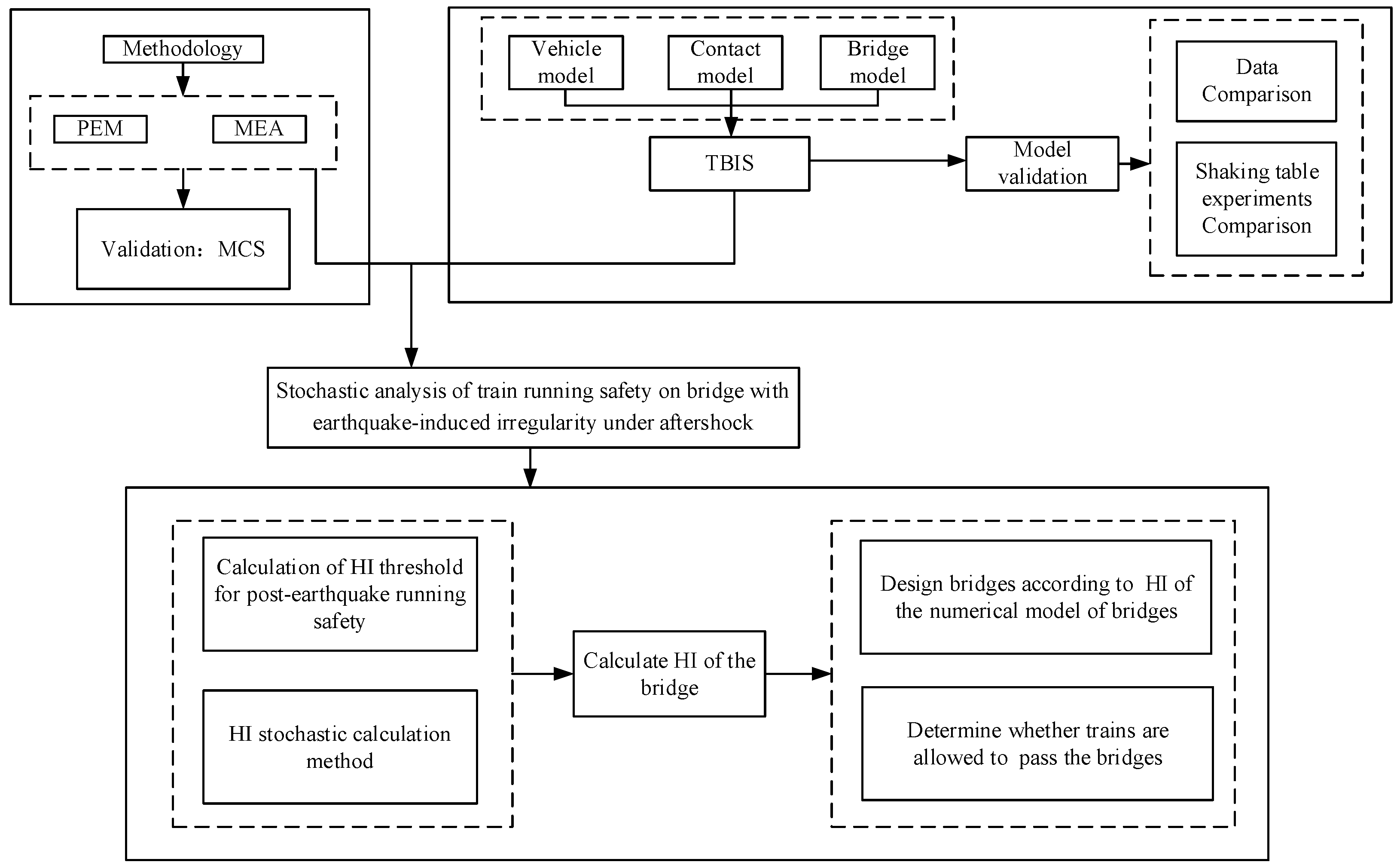
Figure 2.
Earthquake-induced irregularity samples. (a): Rail irregularity samples. (b): TSM. (c): KS test result. (d): KLE.
Figure 2.
Earthquake-induced irregularity samples. (a): Rail irregularity samples. (b): TSM. (c): KS test result. (d): KLE.
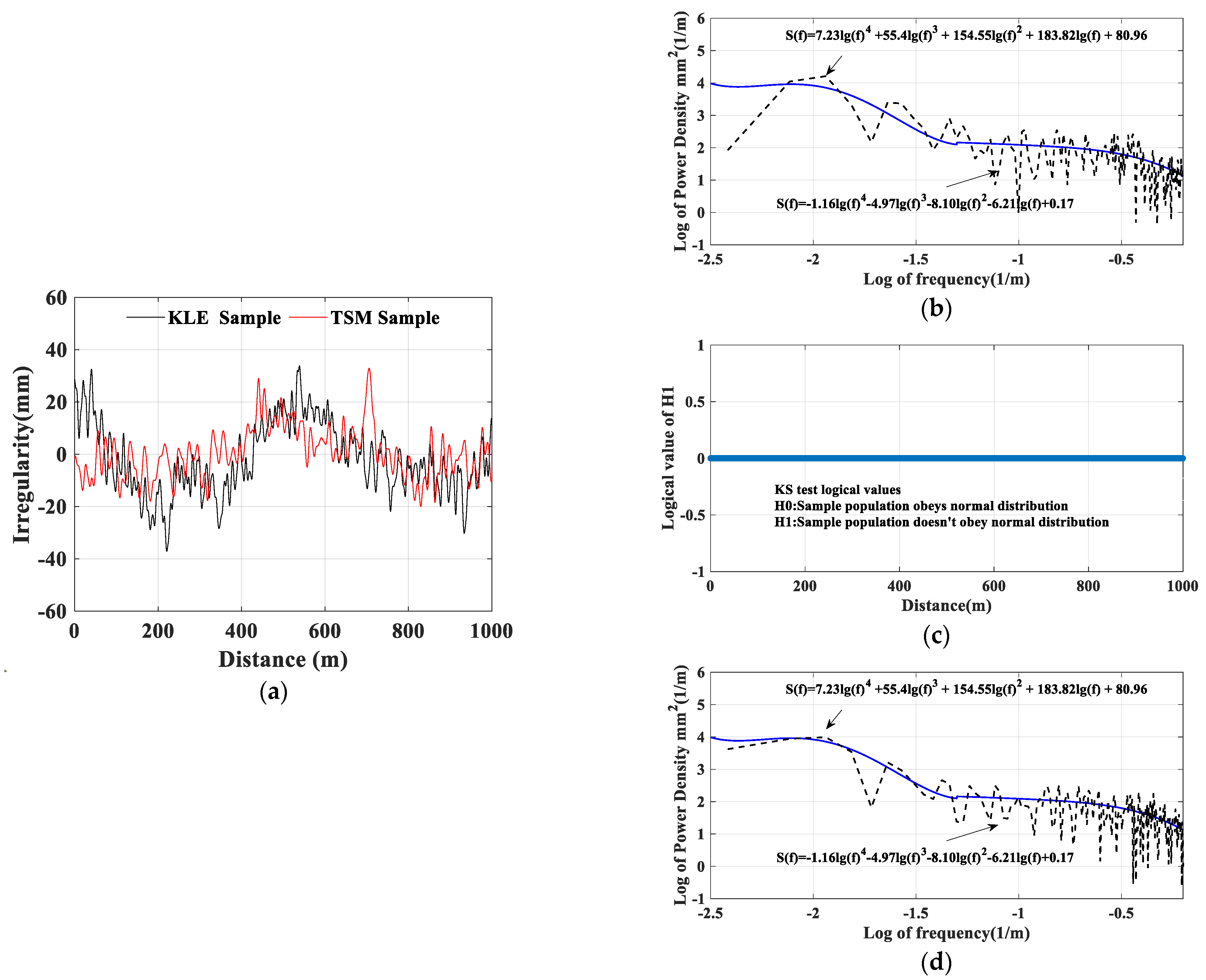
Figure 3.
The main steps of dynamic response analysis of the TBIS. (a): The main steps of dynamic response analysis of the TBIS with single random variables. (b): The main steps of dynamic response analysis of the TBIS with multiple random variables.
Figure 3.
The main steps of dynamic response analysis of the TBIS. (a): The main steps of dynamic response analysis of the TBIS with single random variables. (b): The main steps of dynamic response analysis of the TBIS with multiple random variables.

Figure 4.
Diagram of bridge.
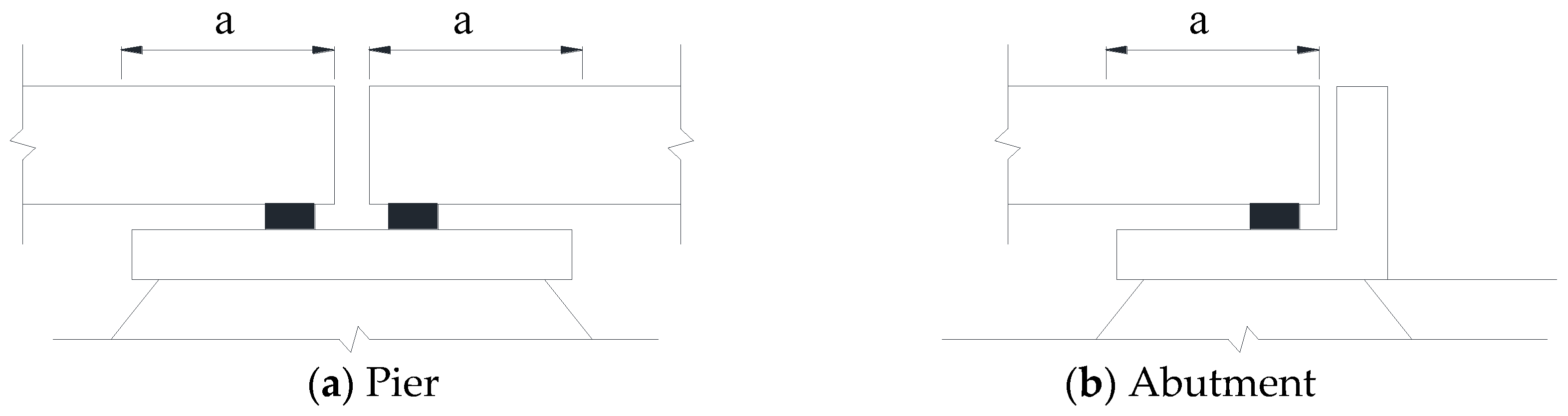
Figure 5.
Knife edge contact model.

Figure 6.
TBIS model validation. (a): Derailment coefficient comparison results. (b): 0.8 Hz, 105 mm amplitude sine wave excitation.
Figure 6.
TBIS model validation. (a): Derailment coefficient comparison results. (b): 0.8 Hz, 105 mm amplitude sine wave excitation.
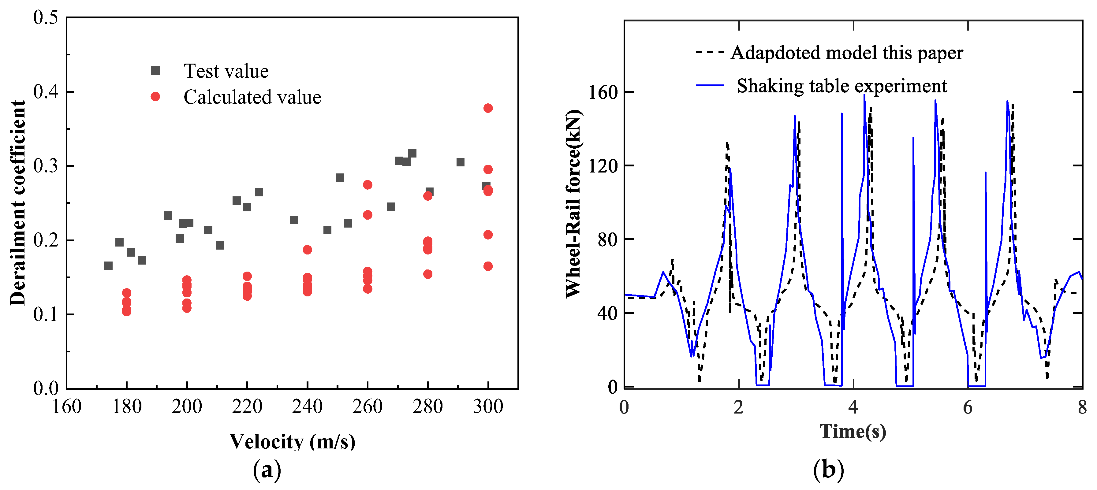
Figure 7.
(a): Horizontal acceleration of bridge midspan; (b): Horizontal acceleration of carbody; (c): PSD of horizontal acceleration of carbody.
Figure 7.
(a): Horizontal acceleration of bridge midspan; (b): Horizontal acceleration of carbody; (c): PSD of horizontal acceleration of carbody.
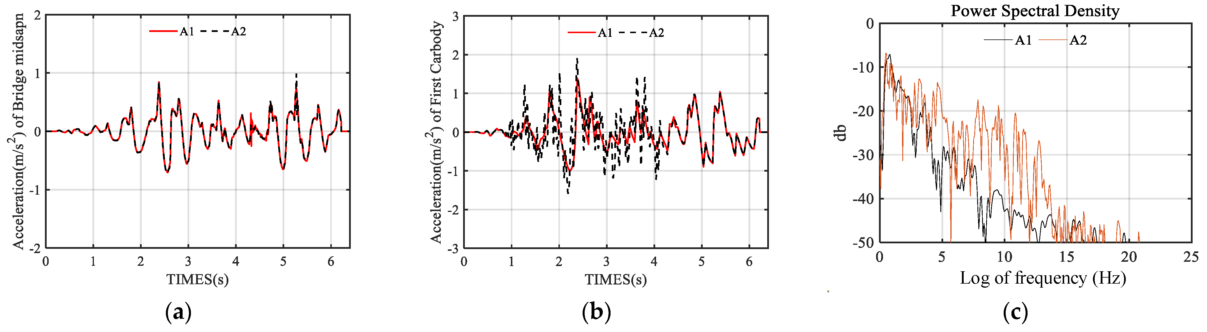
Figure 8.
Comparison between MCS and PEM. (a): Comparison of bridge responses, (b): Comparison of train responses.
Figure 8.
Comparison between MCS and PEM. (a): Comparison of bridge responses, (b): Comparison of train responses.

Figure 9.
MEA validation. (a): Confidence interval of MEA and MCS-1000 and heat map. (b): MEA with 7 degrees. (c): MEA with 8 degrees. (d): MEA with 15 degrees.
Figure 9.
MEA validation. (a): Confidence interval of MEA and MCS-1000 and heat map. (b): MEA with 7 degrees. (c): MEA with 8 degrees. (d): MEA with 15 degrees.
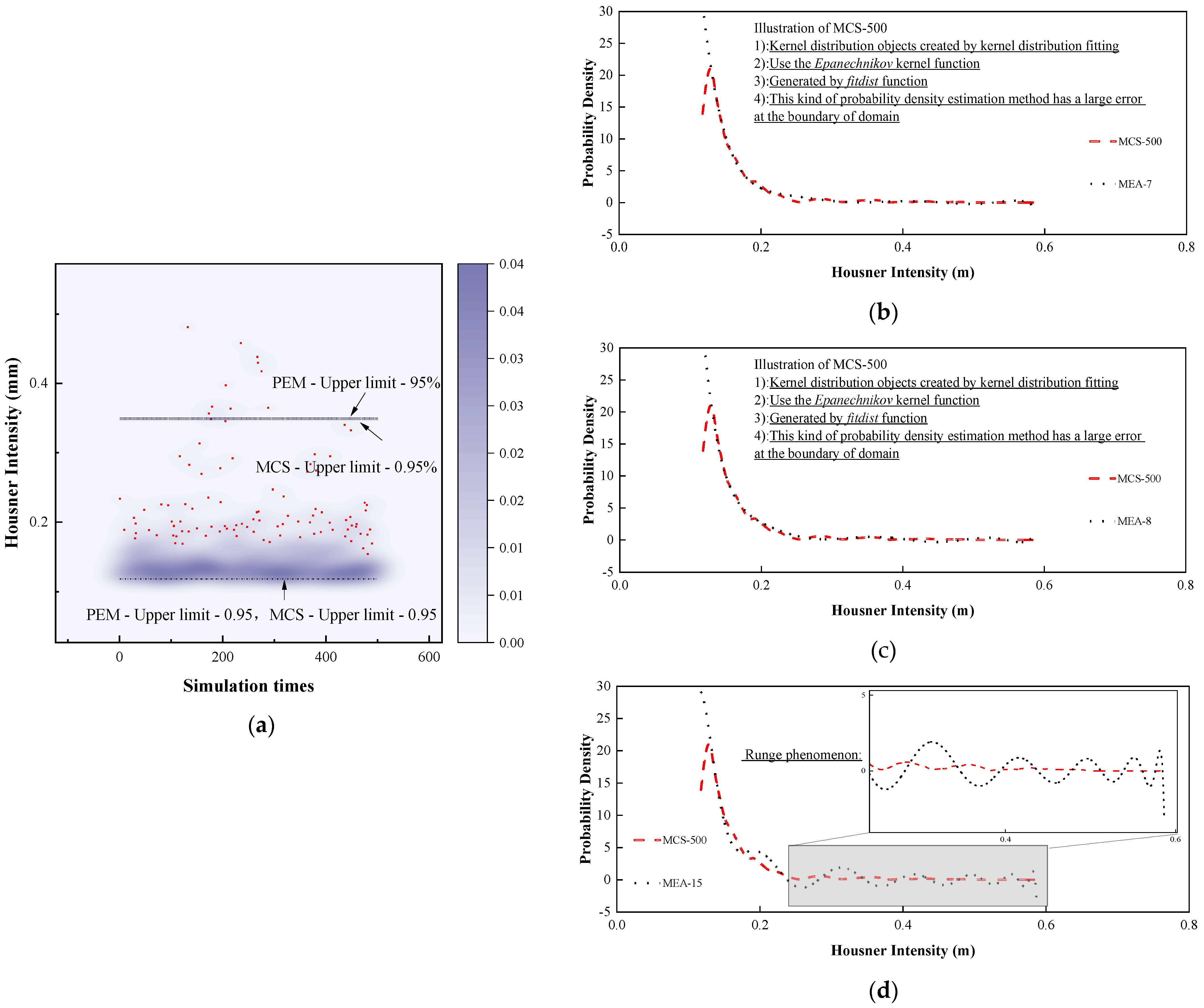
Figure 10.
Flow chart of calculation.
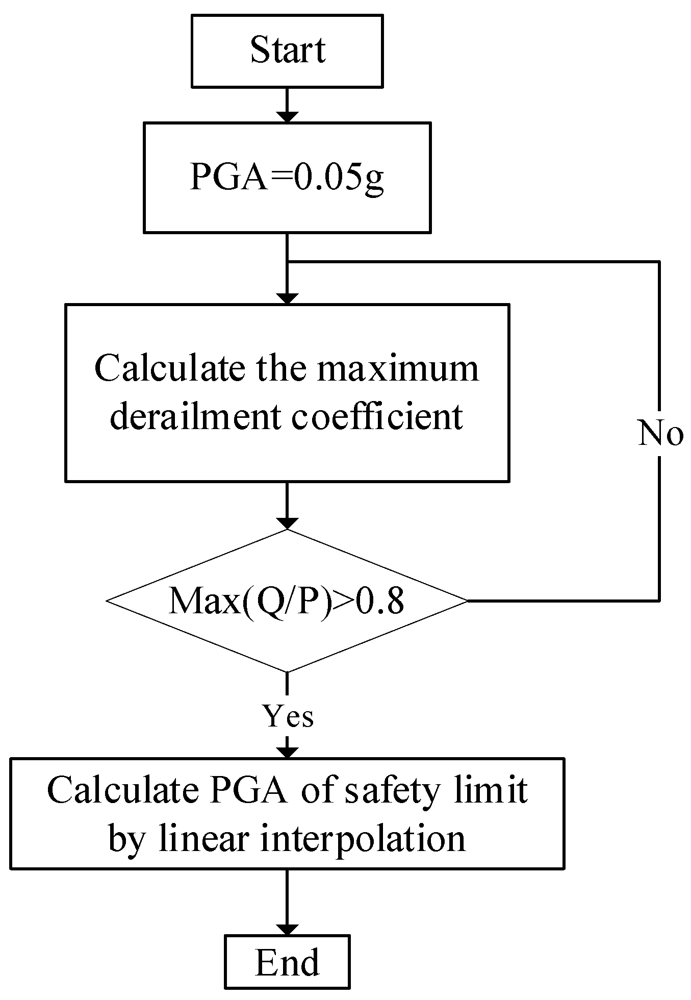
Figure 11.
Calculation of HI.
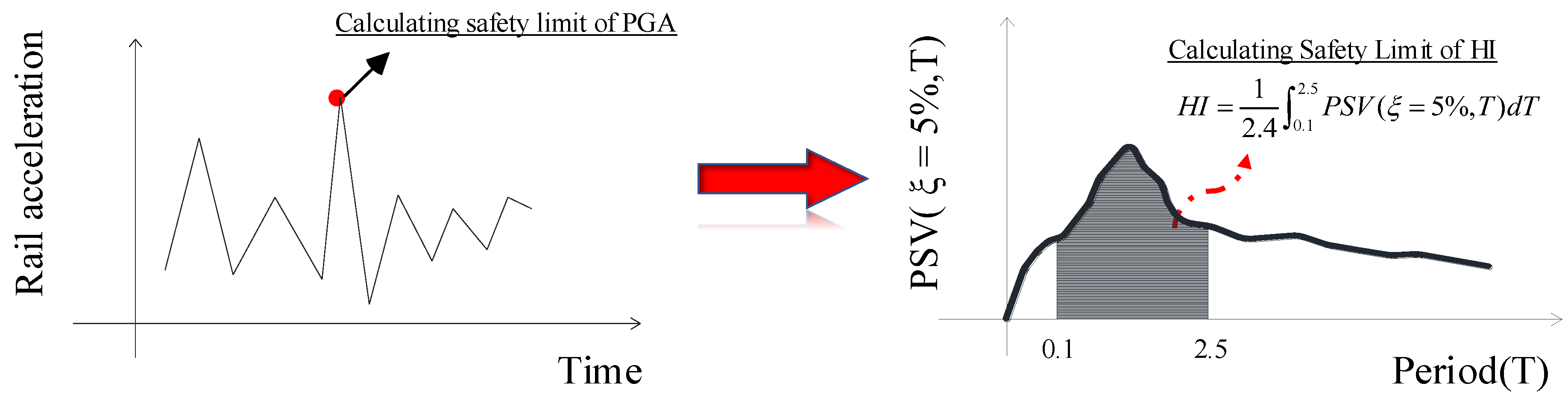
Figure 12.
Safety limit and the maximin derailment coefficient.


Table 1.
CRH2 suspension lateral block.
| Compression (m) | 0 | 0.02 | 0.03 | 0.035 |
|---|---|---|---|---|
| Force (N) | 0 | 0 | 2107 | 5596 |
Table 2.
Confidence intervals.
| 0.9 | 0.8 | 0.7 | 0.6 | |||||
|---|---|---|---|---|---|---|---|---|
| Upper | Lower | Upper | Lower | Upper | Lower | Upper | Lower | |
| MEA | 0.3542 | 0.1184 | 0.2062 | 0.1210 | 0.1906 | 0.1228 | 0.1773 | 0.1246 |
| MCS | 0.3402 | 0.1182 | 0.2010 | 0.1203 | 0.1864 | 0.1218 | 0.1769 | 0.1233 |
Note: represents the confidence level of the confidence intervals.
Table 3.
Distribution.
| Variable | Symbol | Distribution | Mean Value | Std.D | Reference |
|---|---|---|---|---|---|
| Young’s modulus | Y.M | Gaussian | 34.51 GPa | 2.0706 GPa | [20] |
| Density | Den | Gaussian | [20] | ||
| Mass trains | Gaussian | 44 t | 2.2 t | [20] |
Table 4.
COVs of different indexes.
| Number | Name | COV |
|---|---|---|
| 1 | Sa-0.2 | 7.59539 |
| 2 | Sa-1.0 | 4.50385 |
| 3 | Sa-T1 | 3.87779 |
| 4 | Sv-T1 | 3.8068 |
| 5 | Sd-T1 | 3.78743 |
| 6 | PSA | 3.78743 |
| 7 | PSV | 3.5809 |
| 8 | PSD | 3.39373 |
| 9 | AI | 8.63451 |
| 10 | CAV | 3.41955 |
| 11 | VSI | 3.64544 |
| 12 | HI | 2.81931 |
Publisher’s Note: MDPI stays neutral with regard to jurisdictional claims in published maps and institutional affiliations. |
© 2022 by the authors. Licensee MDPI, Basel, Switzerland. This article is an open access article distributed under the terms and conditions of the Creative Commons Attribution (CC BY) license (https://creativecommons.org/licenses/by/4.0/).
Share and Cite
MDPI and ACS Style
Tan, J.; Xiang, P.; Zhao, H.; Yu, J.; Ye, B.; Yang, D. Stochastic Analysis of Train Running Safety on Bridge with Earthquake-Induced Irregularity under Aftershock. Symmetry 2022, 14, 1998. https://doi.org/10.3390/sym14101998
AMA Style
Tan J, Xiang P, Zhao H, Yu J, Ye B, Yang D. Stochastic Analysis of Train Running Safety on Bridge with Earthquake-Induced Irregularity under Aftershock. Symmetry. 2022; 14(10):1998. https://doi.org/10.3390/sym14101998
Chicago/Turabian StyleTan, Jincheng, Ping Xiang, Han Zhao, Jian Yu, Bailong Ye, and Delei Yang. 2022. "Stochastic Analysis of Train Running Safety on Bridge with Earthquake-Induced Irregularity under Aftershock" Symmetry 14, no. 10: 1998. https://doi.org/10.3390/sym14101998
Note that from the first issue of 2016, this journal uses article numbers instead of page numbers. See further details here.