

The Golden Ratio in Nature: A Tour across Length Scales

Molecular Therapeutics and Formulation, School of Pharmacy, University of Nottingham, Nottingham NG7 2RD, UK
*
Author to whom correspondence should be addressed.
Symmetry 2022, 14(10), 2059; https://doi.org/10.3390/sym14102059
Submission received: 15 August 2022
/
Revised: 4 September 2022
/
Accepted: 23 September 2022
/
Published: 3 October 2022
(This article belongs to the Section Physics)
Abstract
:The Golden ratio is an irrational number that has a tendency to appear in many different scientific and artistic fields. It may be found in natural phenomena across a vast range of length scales; from galactic to atomic. In this review, the mathematical properties of the Golden ratio are discussed before exploring where in nature it is claimed to appear; beginning at astronomical scales and progressing to smaller lengths, until reaching those of atomic and quantum physics. For each phenomenon discussed, the evidence for the presence of the Golden ratio is assessed. In making such a tour across length scales, it is illustrated just how prevalent this single number is within the natural universe.
1. Introduction
The Golden ratio, has fascinated people of multiple disciplines, sciences and arts alike, for centuries [1,2,3,4,5,6,7,8]. The earliest known definition for appeared in Euclid’s Elements in approximately 300 BC. The definition involves dividing a line segment into two parts, of lengths A and B as shown in Figure 1, such that the ratio of the larger part, A, to the smaller part, B, equals the ratio of the whole segment to the larger part,
This definition is an example of self-similarity. This means that the line segment is similar to parts of itself, with A being to what B is to A. If a similar division was to be made to length A, then the larger part of that cut would have length B. The common ratio is the Golden ratio, the exact value of which can be found by setting equal to in Equation (1) to give a quadratic equation,
The positive solution of this quadratic is the Golden ratio,
The other solution gives,
The second solution has the same decimal expansion as the first. An interesting property of the Golden ratio is that its reciprocal can be obtained by subtracting one, i.e.,
The Golden ratio seems to possess an almost mythical reputation compared to other numbers, as can be intuited from its name. Another name given to this number is the Divine Proportion, going back to the work of Italian mathematician Luca Pacioli, Divina proportione, in 1509. This reputation is fuelled by claims (often with dubious evidence) that explicitly occurs in certain famous architectural and artistic works, ranging from the Great Pyramid in Egypt and the Parthenon in Greece, to the paintings of Renaissance polymath Leonardo da Vinci (who illustrated Pacioli’s work) [9].
Despite these misconceptions, has been found to legitimately occur in a diverse range of natural phenomena, at length scales varying from the atomic to those of galaxies. The purpose of this paper is to discuss a selection of these phenomena and to assess the evidence suggesting a link to the Golden ratio. For the purposes of this study, a natural phenomenon is considered to be linked to the Golden ratio if two conditions are satisfied: the existence of observational or experimental evidence of , and a rigorous theoretical justification explaining its presence. Where one exists without the other, any evidence shall be considered to be inconclusive.
In Section 2, the mathematical properties of are explored further in the context of its irrationality. This is followed in Section 3 by a discussion of the various occurrences of in science, starting at the galactic length scale and proceeding to smaller lengths until reaching the atomic scale. Where appropriate, some of these occurrences of are explained in terms of the properties discussed in Section 2. Each subsection ends by summarising the evidence for a link to the Golden ratio, concluding for each case whether such a link exists according to the criteria given above.
2. The ‘Most Irrational’ Number
The decimal expansion of never ends, and it never repeats. This is a consequence of the fact that is an irrational number, which means it cannot be expressed as a ratio of two integers. is sometimes referred to as the ‘most irrational’ number, a statement that strictly speaking makes no sense, as a number can either be rational (i.e., can be expressed as a ratio of two integers) or irrational (i.e., not rational). The reason for saying that is ‘more irrational’ than any other irrational number lies in the attempt to approximate it using rational numbers.
The approximation of irrational numbers using rational numbers is the subject of a branch of mathematics known as Diophantine approximation. Any irrational number can be approximated using a ratio of integers, for example, , the ratio of a circle’s diameter to its radius, can be approximated to two decimal places by the simple fraction . Any real number (rational or irrational) may be expressed using a continued fraction,
For a rational number, there are a finite number of integers, , and so the continued fraction eventually ends. On the other hand, an irrational number has a never ending continued fraction expansion. An approximation to an irrational number can be found by finding a finite number of its values. In the case of the Golden ratio, each of the values are equal to one. The resulting approximations from this are ratios of numbers from the Fibonacci sequence. This famous sequence is defined by setting the first two terms both equal to one, and then each subsequent term is equal to the sum of the previous two. The first few Fibonacci numbers are,
If a particular number from this sequence is divided by the previous term, the result is an approximation to . As the chosen Fibonacci number grows larger, the approximation to improves, as shown in Figure 2. For any irrational number, x, the continued fraction expansion may be used to obtain a sequence of rational approximations (where p and q are, respectively, the numerator and denominator of the approximation). As q increases, the approximation becomes closer to the irrational number. To account for this when measuring how well the irrational number is approximated, one can multiply the difference between x and by . A result known as Dirichlet’s approximation theorem shows that there exist infinitely many rational approximations that satisfy the inequality,
This provides an upper bound on how good the approximation can be. For any choice of x, the smallest possible value for this upper bound is given by Hurwitz’s theorem [10],
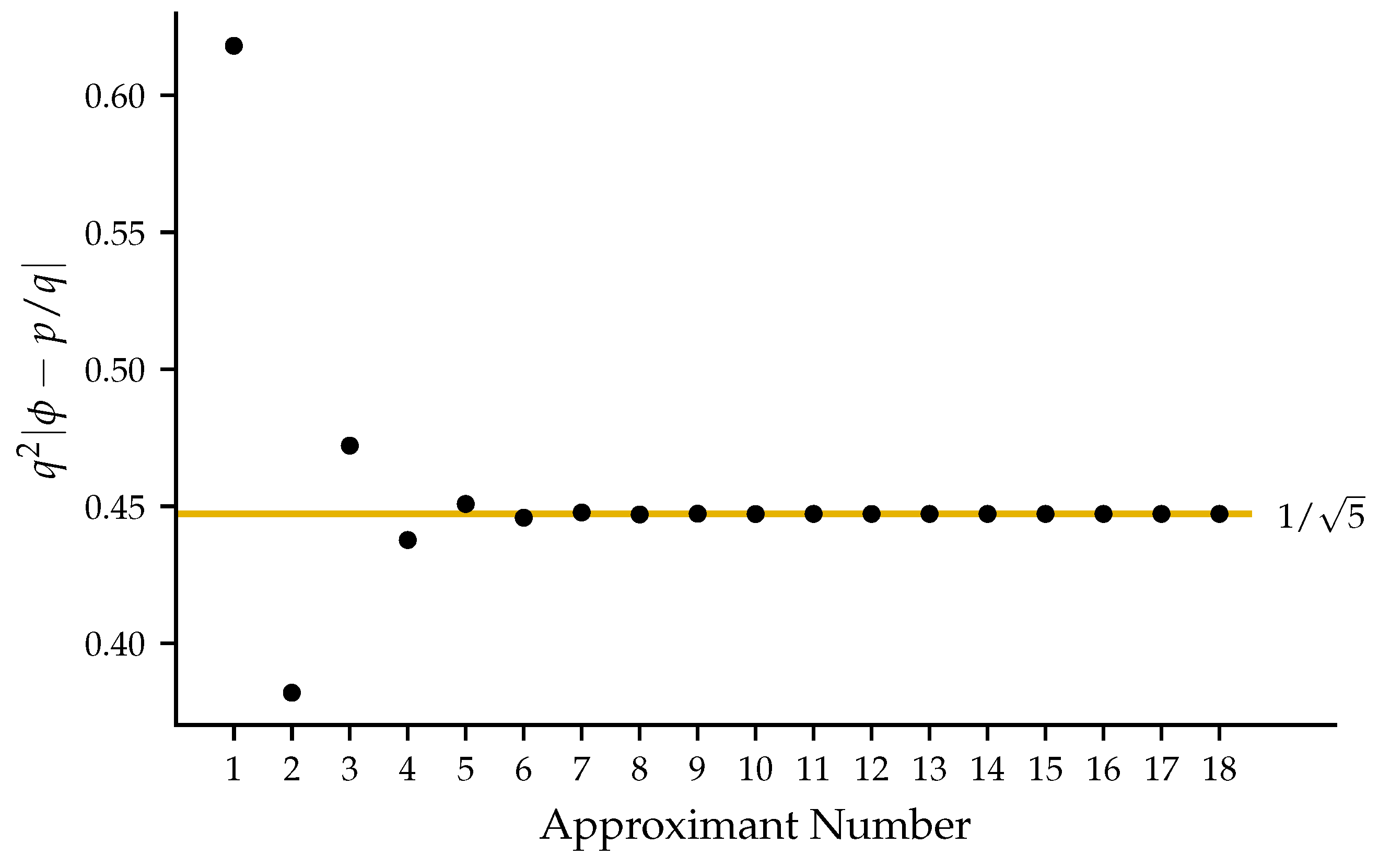
In addition, equality holds only if (or any other number whose continued fraction expansion contains infinitely many 1’s). Figure 3 shows how (this may be interpreted as a relative error) varies as more terms in the continued fraction expansion are included. There is a rapid convergence towards . In other words, for most rational approximants of , the relative error term is close to the upper bound. Since for any other (non-equivalent) number, the upper bound is smaller, the rational approximants of the Golden ratio and its equivalents are worse than for any other number. It is for this reason that is often referred to as the ‘most irrational’ number.
3. The Golden Ratio in Nature
A wide variety of natural phenomena can be linked to the Golden ratio, and these occur on length scales ranging from the atomic to the astronomical. Here, some such phenomena shall be explored, starting at the astronomical scale and progressing to smaller scales.
3.1. Spiral Galaxies
The largest length scale on which has been observed is that of galaxies, which comprise of billions of stars bound by gravity. Many galaxies are characterised by their visually striking spiral arms [11]. A commonly used mathematical model for these arms is the logarithmic spiral, shown in Figure 4, for which the shape remains the same as size increases due to a constant pitch angle. The equation for the logarithmic spiral is,
where r and are plane polar coordinates, a is a constant parametrising size, and k is given by,
where pitch angles and are defined by Figure 4.
In studying a sample of 350 galaxies, it was found by Block and Fairall [12] that the pitch angle (in their paper, defined as the angle) for galactic spiral arms averages at approximately . The following year, Oldershaw [13] pointed out that this pitch angle yields a special logarithmic spiral known as the Golden spiral, whose radius grows by a factor of every time the turn angle, , increases by . To show this, one can take Equation (10) for two points on the spiral, at radii and , separated by a turn angle of , to give,
and
Taking the natural logarithm of both sides and rearranging gives,
Using galactic pitch angle data of 50 spiral galaxies, as measured by Savchenko and Reshetnikov [14], the pitch angle distribution shown in Figure 5 was generated. As can be seen, the peak appears close to . The mean for this sample is with a standard deviation of , which is just under a quarter of .
It should be noted that real spiral galaxies are not perfect logarithmic spirals. For real galaxies, the pitch angle can vary as radius increases. The work of Savchenko and Reshetnikov shows that galactic pitch angles () decrease as r increases (the values used to plot the distribution are averages) [14]. Nevertheless, it is interesting that by approximating spiral galaxies using a simple geometric shape in the logarithmic spiral, the single parameter used to describe the shape appears to peak close to a value associated with the Golden spiral.
Due to the small sample size considered here, the bin widths in Figure 5 are wide (comparable with the standard deviation of the sample). As a result, it is unclear whether the distribution really peaks at the Golden pitch angle. Combined with the lack of a theoretical justification, one may conclude that there is insufficient evidence for the Golden ratio in spiral galaxies.
The Logarithmic Spiral
Other than galaxies, there exist a number of natural phenomena that can be described by logarithmic spirals. Examples include the flight paths of insects [16] and birds [17], nautilus shells and tropical cyclones [18]. Such examples are often mentioned in connection with the Golden ratio (see for example, Reference [5]). Quite often however, the spirals in question are not necessarily Golden [19]. The logarithmic spiral is so often connected with the Golden ratio because the Golden rectangle (i.e., a rectangle with Golden aspect ratio) can be used to construct an approximate logarithmic spiral, as shown in Figure 6. One can split a Golden rectangle by making a Golden cut along the long edge to form a square and a smaller Golden rectangle. This can then be performed on the smaller rectangle, and iterated to generate yet smaller rectangles. An approximate logarithmic spiral can then be produced by drawing quarter circular arcs to connect opposite corners of the squares.
While the above example of spiral galaxies does appear to distribute about a pitch angle close to that of the Golden spiral, a case that does not is that of the nautilus shell [20,21,22]. Despite this, the image of the nautilus shell has become synonymous with the Golden ratio, as evidenced by such an image being featured on the front cover of many books on the Golden ratio (for example, References [3,4,5,6,7]).
The case of the nautilus shell is a cautionary example that shows the need to be careful when encountering claims that the Golden ratio appears in some phenomenon. On the one hand, there may be an element of misunderstanding, such as confusion over the Golden spiral and the more general logarithmic spiral. On the other hand, too much scepticism could lead to legitimate occurrences of in nature being overlooked.
3.2. Variable Stars
One apparently legitimate appearance of in nature may be found in a particular class of variable star. Many stars, such as the Sun, have a luminosity that remains roughly the same over time. Some stars however, have a variable luminosity, caused by periodic changes in pressure. One such class of star are the RR Lyrae variables (named after the variable star RR Lyrae), which are useful to astronomers as standard candles. Some of these variable stars pulsate with multiple frequencies.
Using data from the Kepler space telescope, Lindner et al. studied four RR Lyrae variable stars with pulsation frequencies found to be in the Golden ratio [23]. It has been noted that many variable stars of multiple frequencies have frequency ratios between 0.6 and 0.64 [24]. Lindner et al. found that these stars exhibit ‘strange non-chaotic dynamics’, meaning that they have fractal behaviour without showing chaotic behaviour. This is a highly non-trivial observation since fractal dynamics is often associated with chaos. These stars are the first discovered natural phenomena to show this form of dynamics, which was first discussed by Grebogi et al. in 1984 [25]. Other variable stars, with commensurate pulsation frequencies were also studied, and these did not exhibit strange non-chaotic behaviour.
Theoretical studies of simple non-linear systems by Lindner et al. (crudely modelling a variable star) also revealed Golden behaviour [26]. This suggests that the observed variable star behaviour may be a universal feature of such non-linear systems. The difficulty of approximating by rational numbers is of importance in the models considered in Reference [26], and so they are related to the infinite continued fraction formula for (i.e., Equation (6) with all ). An equivalent expression for the Golden ratio exists, in terms of infinitely nested square roots [27,28]
An investigation by Kutsenko regarding the details of how this expression converges has revealed fractal behaviour [29], providing another link between the Golden ratio and non-linear dynamics.
While observations are limited to a small number of stars, the appearance of the Golden ratio is supported by theoretical predictions (albeit of simplified models). As Golden behaviour emerges in both the theoretical and observational treatment of RR Lyrae stars, it seems as though they are related to the Golden ratio.
3.3. Planetary Orbits
Focusing now on the orbits of planets around a star, an interesting manifestation of Fibonacci numbers and the Golden ratio may be found in the Solar System. It has been noted that the mean distances of the planets from the Sun approximately relate to each other according to the Golden ratio [30,31]. The ratios of successive orbital periods have been found to be preferentially closer to Fibonacci ratios than to other fractions; not only for planets in the Solar System, but also for satellites of the gas giants and even in exoplanetary systems [32].
Dynamics simulations can be used to verify that the orbital periods of the planets (the time taken for each planet to complete one orbit of the Sun) relate to each other according to Fibonacci numbers. In such a simulation (A Python implementation of this simulation is available at http://doi.org/10.17639/nott.7230, Accessed on 27 September 2022), the Sun and eight planets interacted via gravity, and the simulated time was days, which is approximately 1630 Earth years. Inspired by Reference [31], this time was chosen as it is about the time taken for Mercury to complete 6765 orbits, with 6765 being the twentieth Fibonacci number. The number of orbits made by each planet in this time was recorded from the simulation, the results of which are shown in Table 1. Each planet completes a number of orbits approximately equal to a Fibonacci number, with the exception of Mars and Neptune, which nonetheless do complete a multiple of a Fibonacci number of orbits.
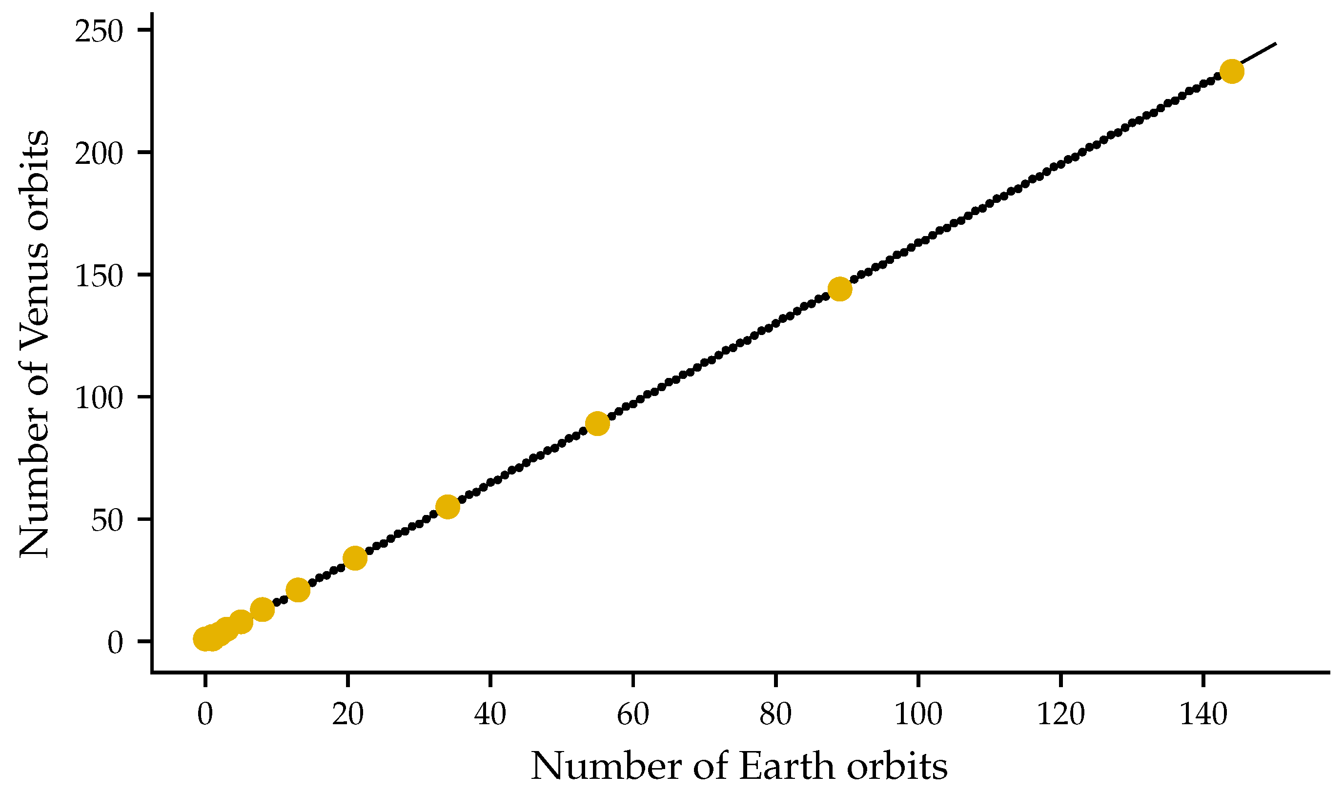
This shows a clear link between planetary orbits and the Fibonacci sequence, therefore suggesting that the ratios between the orbital periods are close to multiples of the Golden ratio. In particular, can be most clearly found when considering the orbits of Earth and Venus. Starting from a configuration where the Sun, the Earth and Venus are co-linear, after eight Earth years this co-linear state (known as a synodic conjunction) occurs five times (with being a Fibonacci ratio), as shown by the intersections in Figure 7, which plots the angular position in the orbit of the two planets against time. Furthermore, if the number of orbits made by Venus is plotted against the number of Earth orbits as in Figure 8, the relationship is linear for long times (i.e., over multiple years) with Fibonacci numbers plotted against the previous terms in agreement with this line. Performing linear regression on this data yields a slope of .
The KAM Theorem
An explanation of why the ratio of planetary orbital periods coincides with is presented by the KAM (Kolmogorov–Arnold–Moser) theorem [33,34]. This theorem applies to integrable (i.e., the equations of motion can be analytically solved) dynamical systems that are subject to a small non-linear perturbation. For example, the motion of a single planet around a star due to gravitation is an integrable system, while the effect of an additional planet is a perturbation. The evolution of a dynamical system can be represented as a trajectory in phase space, the space of all possible states of the system. For any integrable system, this trajectory is confined to the surface of an n-dimensional torus embedded in the -dimensional phase space (where n is the number of independent degrees of freedom of the system) [35]. These surfaces are known as invariant tori because a trajectory that begins on such a surface remains on the surface for all values of time. The exact torus on which the trajectory resides is determined by the initial conditions of the system. Given that the phase space trajectory of an integrable system lies on an n-dimensional invariant torus, the dynamics of the system can be described by the combined effect of the n periodic motions along each independent direction of the torus. Thus, for , there are n natural frequencies, , on the torus. The ratios, , are called the winding numbers of the torus. In the case where each winding number is rational, the trajectory is periodic, whereas if any winding numbers are irrational, then the trajectory eventually covers every point of the torus—in which case the trajectory is quasiperiodic.
According to the KAM theorem, under a small perturbation to an integrable system, some of these tori are deformed but still remain as invariant surfaces, while others are destroyed and so the trajectory is no longer restricted. A stronger perturbation to the system results in the destruction of more invariant tori. The surviving tori have frequencies whose ratios are ‘sufficiently irrational’. A consequence of this is that dynamical systems with frequencies of an irrational ratio are more resilient to perturbations [36]. Since the Golden ratio is the ‘most irrational’ number, a Golden frequency ratio provides the most resistance to perturbations. Thus, in the case of the Solar System, having orbital periods related by maximises stability.
This theoretical explanation provides a clear reason for the Golden ratio to be present in planetary orbits. Moreover, this explanation makes use of the properties of as an irrational number. Supported by observational evidence that Fibonacci numbers approximately occur in the Solar System, it is clear that the Golden ratio plays a profound role in planetary orbits.
3.4. Phyllotaxis
Observations of are not restricted to only celestial objects. A commonly noted Earthly case is that of phyllotaxis [37,38,39], the arrangement of leaves on a stem, which form spiral patterns. In such spirals, the rotational angle around the stem from leaf to leaf is approximately , the angle that divides the circumference of a circle into the Golden ratio. This observation was first reported in the early nineteenth century by Schimper and by Braun, in the form of the ratios of small Fibonacci numbers (see Reference [40] for additional historical references). The reason for this is that the ‘maximally irrational’ property of provides the least chances for leaves to be positioned directly above each other, and thus each leaf receives the maximum possible amount of sunlight.
A mathematically rigorous explanation for why the Golden angle is optimal is offered by Bergeron and Reutenauer [41]. In their paper, a simple model of ‘buds’ growing along a helix on a cylindrical ‘plant’ is studied. Around each bud, a disk is placed with diameter such that no overlap occurs. Then it is shown that a quantity representing the ‘capacity’ of the plant (i.e., the ability for the plant to grow the most number of buds using minimal disk area) is optimised when the rotational angle is Golden. As with the KAM theorem, the proof of this makes use of the irrationality of in the sense discussed above (see Section 2).
In light of a mathematical proof for the optimality of the Golden angle, along with observational evidence of the Golden angle that spans nearly two centuries; one may conclude that the Golden ratio is strongly linked to Phyllotaxis.
3.5. The Ultimatum Game
In game theory, the branch of mathematics devoted to understanding strategic decision making when two ‘players’ interact, the Golden ratio appears in the ultimatum game, first described by Güth et al. [42]. In this game, one player has a set amount of some resource (money, for example), and must offer a share of this to a second player. If the second player accepts, then the resource is divided according to the offer. If they reject the offer, then both players leave empty handed. One might think that the best possible strategy for the first player is to make the smallest possible (non-zero) offer, while the second player’s best strategy is to accept this. However, in practice, this is not found to be the actual outcome. The most likely accepted offers tend to be around (or close to the inverse of the Golden ratio) [43,44]. It was suggested by Schuster [45] (with an argument based on continued fractions) that the solution to the ultimatum game is to make an offer such that the proportion of the second player’s share to the first player’s equals that of the first player to the whole, i.e., the Golden section. This solution could be interpreted as the fairest possible trade-off given an asymmetric situation. The Economic Harmony theory of Suleiman [46] predicts that the split between players should be the Golden ratio, when considering the ratio between actual and desired pay-off. In addition, Suleiman showed that the agreement between experimental data and the proposed Golden solution is statistically significant [46].
The ultimatum game has been applied to a wide range of situations, including that of human walking [8]. In this case, there are two phases: the stance (when both feet are on the ground) and swing (when a foot leaves the ground). The most common ratio between the times spent in each of these phases was found by Iosa et al. to be Golden. From the game theory perspective, the Golden ratio provides the optimal compromise between continued motion and stability of the walker.
The approximate split of 60% to 40% observed in many experimental studies, along with two independent theoretical treatments predicting and explaining a Golden solution, suggest a strong link between the ultimatum game and the Golden ratio.
3.6. The Human Body
Knowing that the Golden ratio plays a role in human walking, one might ask whether it also appears in the human body? The answer to this question is that it might, and in a variety of situations including the heart and the brain, which are both considered here.
3.6.1. The Heart
The work of Henein et al. [47] shows three cases of present in the human heart. Their work used images obtained by ultrasound and computerised axial tomography (CAT) scans, as well as the resting phase of the heart cycle. Firstly, it was found that vertical and transverse measurements of the left ventricle (one of the chambers of the heart) are in the Golden ratio. Secondly, the annulus dimensions in the mitral valve (located between the left ventricle and left atrium) were also found to be in the Golden ratio. Thirdly, the angle between the right ventricular inlet axis and the outflow tract axis was found to be close to the Golden angle, . For all three of these measurements, there was an observed deviation from when the heart was not healthy. This means that such measurements could be used as a way to identify when the heart deviates from normality.
3.6.2. The Brain
A recent discovery is that occurs in the dimensions of the human skull. The work of Tamargo and Pindrik [48] took CAT scanned images of human skulls and considered three points; the nasion (where the frontal bone meets the nasal bones), the inion (a protuberance at the back of the skull) and the bregma (a point at the top of the skull where the frontal and parietal lobes meet). Taking the arc joining the nasion and inion, and dividing it into two sections separated by the bregma, Tamargo and Pindrik found that the resulting sections are Golden, i.e., the bregma makes a Golden cut to this arc. They also found that the equivalent skull dimensions of some other mammals, such as monkeys, rabbits, dogs, lions and tigers, have differing ratios. Furthermore, these ratios appear to approach as the species becomes more sophisticated.
For both the human heart and brain, there exists observational evidence that the Golden ratio is present in their proportions. However, in both cases there is no theoretical explanation of why this might be so. In the absence of this, the existing evidence is circumstantial; enough to suggest that the Golden ratio might be present, but not sufficient to prove it.
3.7. Proteins and Amino Acids
With the ubiquity of in various organs of the human body, it seems natural to ask whether appears at smaller biological scales. Recently, the Golden ratio has also been observed at the nanometre scale [49], in the shape of proteins, macromolecules which play a vital role in our existence. The distribution of protein aspect ratios, obtained using calliper measurements from the Protein Data Bank (PDB), are shown in Figure 9. There are two peaks in this distribution, one for prolate (cigar shaped) proteins, and one for oblate (frisbee shaped) proteins. The mode aspect ratio in the prolate case is close to the Golden ratio, while the peak oblate shape is close to its reciprocal.
To help assess whether these aspect ratios distribute about , hypothesis tests were performed on the protein and amino acid data. Following the recommendation of Santos et al. [50], the (two-tailed) t-Student test was used with the test statistic defined as (where a and b are the long and short calliper lengths, with ). In these tests, the null hypothesis is that the distributions are centred around . For a subset of the protein data, taken from the PDBselect database [51], three sets of proteins were tested: oblate, prolate and the whole set. Taking a significance level of one percent, the obtained p-values were: , and . The vanishingly small p-values in the latter two cases imply that the prolate proteins, as well as the entire set, do not distribute around (i.e., the null hypothesis is rejected). In the oblate case, there is not enough evidence to reject the null hypothesis and so there remains the possibility that their peak is Golden.
It was also observed that the amino acids that comprise proteins have aspect ratios that distribute around a value near the Golden ratio. For each residue in the protein dataset (approximately 13 million amino acids), the spheroid of equivalent steric volume to the side chain was calculated. This gives a distribution of aspect ratios for each of the 20 types of amino acid found in proteins. The average aspect ratio (the ratio between the spheroid major axis, a, and minor axis b) for each amino acid type (not including glycine, whose side chain consists of a single hydrogen atom) is shown in Figure 10. It can be seen that the ratios and distribute around a value close to . It can be noted that the average values of and (1.6120 and 1.6808) are quite close to each other, suggesting that the average shape of amino acids is close to Golden. Interestingly, when taking into account the number of residues of each type in the protein data, the average aspect ratio, , drops to about 1.6401 (dash-dotted black line in Figure 10). This can be explained by noting that the three most commonly occurring amino acid types in the protein dataset, alanine (ALA), leucine (LEU) and valine (VAL), have relatively low aspect ratios (all below 1.6). While the weighted average aspect ratio is near to , it should be noted that none of the twenty amino acids themselves have a Golden aspect ratio.
It is an interesting observation that amino acids in proteins have a shape similar to that of the proteins they make up, and that this common aspect ratio coincides with , which is itself defined using the idea of self-similarity. Beyond this coincidence, there is little further evidence suggesting that the Golden ratio is present in proteins. Prolate proteins (and the set as a whole) can be judged as non-Golden based on the result of the hypothesis test above, although it cannot be ruled out that the same holds for oblate proteins. Moreover, there exists no known theoretical reason for proteins or amino acids to have a Golden shape. Therefore, there is not enough evidence to confirm that the Golden ratio is linked to proteins.
3.8. Penrose Tilings and Quasicrystals
In addition to proteins, another example of how atoms can assemble in a self-similar fashion is that of quasicrystals, structures that are ordered in space but are not periodic. A crystal is an ordered arrangement of points, usually with a regularly repeated (i.e., periodic) pattern. A mathematical result known as the crystallographic restriction theorem states that the only allowed rotational symmetries for a crystal are 2, 3, 4 and 6-fold. In other words, a periodic tiling using one of these symmetries can be used to completely fill space. This does not apply to 5-fold, or x-fold (where ) symmetry, meaning for example, that it is not possible to tile two-dimensional space using regular pentagons. In the geometry of the regular pentagon, the Golden ratio appears. As pictured in Figure 11, the diagonal length divided by the side length equals . Thus, the Golden ratio may be associated with five-fold symmetry in a similar way to how the number is associated with circular symmetry.
It was discovered by Penrose that two-dimensional space can in fact be tiled by using a pair of shapes derived from the pentagon [52]. An example of such a tiling, where each tile is one of two types of rhombus, is shown in Figure 12. The Penrose tiling has the property of not being periodic, but yet is self-similar in that finite patches of the tiling are repeated infinitely many times. Furthermore, it is possible to transform a Penrose tiling into another equivalent tiling by applying a particular set of substitution rules to the tiles. The Penrose tiling also exhibits multiple instances of the Golden ratio, as might be expected due to its five-fold symmetry. The Golden ratio is prominent in the geometry of the tiles themselves, and in the limit of infinitely many tiles, the ratio of wide to thin rhombi is .
To see how the Golden ratio appears in the Penrose tiling, it is useful to consider a one-dimensional example of a ‘tiling’, based on the Fibonacci sequence. This example may be constructed by first taking a square lattice in two dimensions, and defining a strip as shown in Figure 13, such that its slope is . If the strip is defined by taking a unit square and moving it along this direction, then the projections of the points within the strip onto the axis parallel to the slope define a series of line segments. It can be seen in Figure 13 that the line segments have one of two lengths, one short and one long. The ratio between these lengths is itself Golden, and the sequence of long and short line segments is equivalent to the Fibonacci sequence. The Penrose tiling can be interpreted as a superposition of five sets of Fibonacci lattices. It was found by Ammann [53,54] that the rhombus matching rules can be formulated by drawing straight lines on the tiles, such that the lines continue when two tiles are placed edge to edge. Figure 14 shows these Ammann lines overlaid on a Penrose tiling. There are five sets of parallel lines, and for each such set of lines, there are two separation lengths. These sets of lines are themselves Fibonacci lattices. The Penrose tiling could thus be viewed as a two-dimensional generalisation of the Fibonacci lattice.
In three dimensions, a forbidden symmetry is that of the icosahedron, a twenty faced regular polyhedron whose geometry features five-fold symmetry and the Golden ratio. The Nobel prize winning discovery by Shechtman of icosahedral symmetry in an aluminium-manganese alloy [55], shows that the crystallographic restriction theorem can be violated by real materials. This shows that a ‘crystal’ structure can be ordered, in that the positions of the tiles are governed by some mathematical prescription, and yet not be periodic. Such structures are known as quasicrystals [56]. There are two types of known thermodynamically stable quasicrystal in three dimensions: polygonal and icosahedral. Polygonal quasicrystals have an axis of either 8, 10 or 12-fold symmetry, with the structure being aperiodic in planes normal to this axis and periodic along it. Icosahedral quasicrystals on the other hand, are aperiodic along all three dimensions. The work of Steinhardt et al. [57,58] considers the icosahedral quasicrystal as the three-dimensional analogue of the Penrose tiling. Icosahedral quasicrystals have been discovered as naturally occurring in samples from the Koryak Mountains in Siberia [59,60,61].
Given the presence of the Golden ratio in the geometry of the icosahedron, it is an interesting observation that this symmetry is the only way to produce a quasicrystal that satisfies quasi-periodicity along all three dimensions, and that it is found in the only known natural quasicrystals. In light of this evidence, there is no doubt that quasicrystals are profoundly linked with the Golden ratio.
3.9. Atomic Bond Lengths
While proteins, amino acids and quasicrystals show possible examples of how many atoms can arrange themselves with geometry described by , the Golden ratio also appears when considering the bonds between pairs of atoms, and can be used as a simple model to predict bond lengths. Using density functional methods, Suresh and Koga obtained a value of nm for the hydrogen-carbon bond lengths in methane [62]. The work of Heyrovska [63,64] was motivated by the fact that this value is close to the Bohr radius, the most probable ground state distance between the proton and electron in the hydrogen atom ( nm), divided by the Golden ratio. That work showed that the Bohr radius can be divided into Golden sections, and , corresponding to the electron and proton, respectively. The ionisation energy for hydrogen in the ground state (i.e., the energy required to separate the electron and proton) can then be written as a difference of two terms based on these distances. This idea has been extended to the case of a covalent bond between two identical atoms. For atoms of type A, the length of such a bond, , can be considered the sum of two radii, and , defined by a Golden cut. Given the covalent bond length for a pair of identical atoms, the values of and may be calculated for the atom of type A. These values can then be used, as in Reference [63], to predict the bond length between two dissimilar atoms.
It was found in Reference [63] that this simple model of bond length shows good agreement with observed bond lengths in examples such as hydrogen halides, alkali halides and metal hydrides. Since the model is based on the Golden ratio, this suggests that Golden behaviour may be present in bond lengths between atoms.
3.10. Black Holes, Quantum Gravity and E8
The two most successful physics theories of the twentieth century are general relativity and quantum mechanics. The former describes gravity and the universe at large scales, while the latter describes the universe at small scales using electromagnetism, the strong nuclear and weak nuclear forces. However, the two theories are notorious for their mutual incompatibility with each other. An example that invokes both theories is that of black holes, which have sufficiently strong gravity that even light cannot escape, and are so compact that quantum effects are important. The study of black holes has revealed multiple instances of the Golden ratio, two of which are discussed here.
A well known example is that of the specific heat capacity of a black hole. Specific heat capacity is defined as the amount of energy that must be added to a unit mass of some object in order to raise its temperature by one unit. Due to a result known as the virial theorem, self-gravitating objects, such as stars, have a negative specific heat, i.e., they become hotter when energy is removed [65]. This happens because as energy is removed, the star contracts and so its constituent particles speed up, increasing the temperature. The same is true of a Schwarzschild black hole, which is a spherically symmetric, non-rotating black hole with zero net charge. When considering a black hole that is rotating, the specific heat capacity can be positive or negative, depending on the angular momentum. It was found by Davies [66] that the transition between negative and positive occurs when the black hole satisfies (using units in which the speed of light and the gravitational constant equal unity),
where M is the mass of the black hole, and J is its angular momentum. Interestingly, a later paper by Davies [67] showed that the same ratio, , equals the inverse Golden ratio, . This latter result has been found to be true, if the ratio of angular momentum and mass is held constant [68].
While the heat capacity example seems physically unlikely (as there is no reason to expect that the angular momentum to mass ratio of a black hole remains constant), Cruz et al. [69] showed that also appears in black hole physics when considering the metric (a mathematical object describing spacetime curvature) of Schwarzschild-Kottler black holes. In particular, appears when considering the null geodesics (i.e., the paths taken by photons) of this metric.
The above paragraphs show that the Golden ratio occurs in certain theoretical treatments of black holes. However, due to the inherent difficulty in observing black holes, there is as yet no evidence that Golden behaviour occurs in real black holes. As a result, it may be concluded that the evidence for black holes being related to is insufficient.
Given the appearance of in black holes, one might question whether it also appears in theories attempting to unify general relativity and quantum theory. Some such attempts involve a mathematical structure known as ‘E8’ [70,71,72], in which may also be found [73]. One way to think of the E8 structure is as a lattice of points, corresponding to the densest way to pack ‘spheres’ in eight-dimensional space [74]. Evidence of an E8 governed phenomenon in nature was found by Coldea et al., with the Golden ratio appearing in a low temperature one-dimensional magnet known as an Ising chain, formed by cobalt niobate [75]. When a critical magnetic field is applied perpendicular to the compound, the spin of each cobalt atom enters a quantum superposition of the up and down states. According to theoretical predictions, in the vicinity of the critical field, the two lightest particles of the chain should have masses in the Golden ratio [76]. In the cobalt niobate experiment, neutron scattering revealed two peaks in energy, interpreted as the two lightest particles of the Ising chain. As the applied field was increased, their ratio approached . As pointed out by Affleck [77], the observation of suggests that E8 underlies this system.
Since the Ising chain is described using E8, its theoretical description contains the Golden ratio. The experimental agreement with this theory thus confirms that the Ising chain is indeed related to the Golden ratio.
While the cobalt niobate experiment is currently the only case of an observed E8 governed system, it shows that the Golden ratio can be found at the quantum scale. The examples discussed above show that there is a tendency for to appear at all length scales, sometimes in surprising places. This tendency for the Golden ratio to appear in such a wide variety of phenomena has even led to suggestions that the Golden ratio is a fundamental constant of nature [78,79].
4. Conclusions
A remarkable number of apparently disparate natural phenomena can be linked to the Golden ratio, and occurrences of this number may be found at multiple length scales, ranging from the galactic to the atomic. Some of these instances; such as planetary orbits, RR Lyrae stars, phyllotaxis, the ultimatum game, Ising chains and quasicrystals stem from the fact that the Golden ratio is, in the sense of Hurwitz’s theorem, the most difficult number to approximate using rational quotients. In such cases, the Golden ratio manifests itself through its rational approximants, given by the ratios of successive Fibonacci numbers. In other cases; including spiral galaxy pitch angles, protein and amino acid shape, atomic bond lengths and black holes, the observations or calculations resulting in the Golden ratio appear coincidental, but may also indicate that some deeper, as yet unknown, explanation exists.
The propensity of this number to appear in unexpected places does however, sometimes lead to misconceptions, such as the idea that the nautilus shell and hurricanes are governed by the Golden spiral. Nevertheless, in exploring just one single number, one may encounter a plethora of fascinating topics from a variety of disciplines. Whenever the Golden ratio (or a nearby value) is encountered in science, there is an exciting opportunity for scientific, philosophical and artistic investigations.
Author Contributions
Conceptualization, C.R.M.; methodology, C.R.M.; software, C.R.M.; investigation, C.R.M.; writing—original draft preparation, C.R.M.; writing—review and editing, C.R.M. and P.M.W.; supervision, P.M.W.; All authors have read and agreed to the published version of the manuscript.
Funding
This work was supported by the Engineering and Physical Sciences Research Council DTP funding (EP/M50810X/1) to the University of Nottingham, and the University of Nottingham, via a PhD studentship to CRM.
Data Availability Statement
Python code implementing the simulation discussed in Section 3.3 is openly available in the Nottingham Research Data Management Repository at http://doi.org/10.17639/nott.7230, Accessed on 27 September 2022.
Conflicts of Interest
The authors declare no conflict of interest.
Abbreviations
The following abbreviations are used in this manuscript:
| KAM | Kolmogorov–Arnold–Moser |
| CAT | Computerized axial tomography |
| PDB | Protein data bank |
References
- Thompson, D.W. On Growth and Form; Bonner, J.T., Ed.; Cambridge University Press: Cambridge, UK, 2014. [Google Scholar]
- Huntley, H.E. The Divine Proportion: A Study in Mathematical Beauty; Dover Publications, Inc.: New York, NY, USA, 1970. [Google Scholar]
- Ghyka, M. The Geometry of Art and Life; Dover Publications, Inc.: New York, NY, USA, 1977. [Google Scholar]
- Dunlap, R.A. The Golden Ratio and Fibonacci Numbers; World Scientific: Singapore, 1997. [Google Scholar]
- Livio, M. The Golden Ratio: The Story of Phi, the World’s Most Astonishing Number; Broadway Books: New York, NY, USA, 2003. [Google Scholar]
- Olsen, S. The Golden Section: Nature’s Greatest Secret; Wooden Books: Glastonbury, UK, 2006. [Google Scholar]
- Corbalán, F. The Golden Ratio: The Mathematical Language of Beauty; National Geographic: Villatuerta, Spain, 2016. [Google Scholar]
- Iosa, M.; Morone, G.; Paolucci, S. Golden Gait: An Optimization Theory Perspective on Human and Humanoid Walking. Front. Neurorobot. 2017, 11, 69. [Google Scholar] [CrossRef] [Green Version]
- Markowsky, G. Misconceptions about the Golden Ratio. Coll. Math. J. 1992, 23, 2–19. [Google Scholar] [CrossRef]
- Benito, M.; Escribano, J.J. An Easy Proof of Hurwitz’s Theorem. Am. Math. Mon. 2002, 109, 916. [Google Scholar] [CrossRef]
- Sparke, L.S.; Gallagher, J.S. Galaxies in the Universe: An Introduction, 2nd ed.; Cambridge University Press: Cambridge, UK, 2007. [Google Scholar]
- Block, D.L.; Fairall, A.P. Some Comments on the Pitch Angle in Spiral Structure. Mon. Notes Astron. Soc. S. Afr. 1981, 40, 43. [Google Scholar]
- Oldershaw, R.L. The Preferred Pitch Angle of Spiral Galaxies; Mathematical and Physical Implications. Mon. Notes Astron. Soc. S. Afr. 1982, 41, 42, Provided by the SAO/NASA Astrophysics Data System. [Google Scholar]
- Savchenko, S.S.; Reshetnikov, V.P. Pitch angle variations in spiral galaxies. Mon. Not. R. Astron. Soc. 2013, 436, 1074–1083. [Google Scholar] [CrossRef]
- Scott, D.W. On optimal and data-based histograms. Biometrika 1979, 66, 605–610. [Google Scholar] [CrossRef]
- Boyadzhiev, K.N. Spirals and Conchospirals in the Flight of Insects. Coll. Math. J 1999, 30, 23–31. [Google Scholar] [CrossRef]
- Tucker, V.A. The deep fovea, sideways vision and spiral flight paths in raptors. J. Exp. Biol. 2000, 203, 3745–3754. [Google Scholar] [CrossRef]
- Moon, Y.; Nolan, D.S. Spiral Rainbands in a Numerical Simulation of Hurricane Bill (2009). Part I: Structures and Comparisons to Observations. J. Atmos. Sci 2015, 72, 164–190. [Google Scholar] [CrossRef] [Green Version]
- Sharp, J. Spirals and the Golden Section. Nexus Netw. J. 2002, 4, 59–82. [Google Scholar] [CrossRef] [Green Version]
- Falbo, C. The Golden Ratio—A Contrary Viewpoint. Coll. Math. J 2005, 36, 123–134. [Google Scholar] [CrossRef]
- Gailiunas, P. The Golden Spiral: The Genesis of a Misunderstanding. In Proceedings of Bridges 2015: Mathematics, Music, Art, Architecture, Culture; Baltimore, MD, USA, 29 July–1 August 2015; Delp, K., Kaplan, C.S., McKenna, D., Sarhangi, R., Eds.; Tessellations Publishing: Phoenix, AZ, USA, 2015; pp. 159–166. [Google Scholar]
- Bartlett, C. Nautilus Spirals and the Meta-Golden Ratio Chi. Nexus Netw. J. 2019, 21, 641–656. [Google Scholar] [CrossRef]
- Lindner, J.F.; Kohar, V.; Kia, B.; Hippke, M.; Learned, J.G.; Ditto, W.L. Strange Nonchaotic Stars. Phys. Rev. Lett. 2015, 114. [Google Scholar] [CrossRef] [PubMed] [Green Version]
- Moskalik, P. Multi-mode oscillations in classical Cepheids and RR Lyrae-type stars. Proc. Int. Astron. Union 2013, 9, 249–256. [Google Scholar] [CrossRef] [Green Version]
- Grebogi, C.; Ott, E.; Pelikan, S.; Yorke, J.A. Strange attractors that are not chaotic. Phys. D 1984, 13, 261–268. [Google Scholar] [CrossRef]
- Lindner, J.F.; Kohar, V.; Kia, B.; Hippke, M.; Learned, J.G.; Ditto, W.L. Simple nonlinear models suggest variable star universality. Phys. D 2016, 316, 16–22. [Google Scholar] [CrossRef] [Green Version]
- Paris, R.B. An Asymptotic Approximation Connected With the Golden Number. Am. Math. Mon. 1987, 94, 272–278. [Google Scholar] [CrossRef]
- García–Caballero, E.M.; Moreno, S.G.; Prophet, M.P. The Golden Ratio and Viète’s Formula. Teach. Math. Comput. Sci. 2014, 12, 43–54. [Google Scholar] [CrossRef]
- Kutsenko, A.A. An Entire Function Connected with the Approximation of the Golden Ratio. Am. Math. Mon. 2020, 127, 820–826. [Google Scholar] [CrossRef]
- Lombardi, O.W.; Lombardi, M.A. The Golden mean in the solar-system. Fibonacci Q. 1984, 22, 70–75. [Google Scholar]
- Tattersall, R. A remarkable Discovery: All Solar System Periods Fit the Fibonacci Series and the Golden Ratio. Why Phi? 2013. Available online: https://tallbloke.wordpress.com/2013/02/20/a-remarkable-discovery-all-solar-system-periods-fit-the-fibonacci-series-and-the-golden-ratio-why-phi/#:~:text=Since%20it%20was%20noticed%20that,structure%20of%20the%20solar%20system (accessed on 22 June 2022).
- Pletser, V. Prevalence of Fibonacci numbers in orbital period ratios in solar planetary and satellite systems and in exoplanetary systems. Astrophys. Space Sci. 2019, 364. [Google Scholar] [CrossRef]
- Broer, H.W. KAM theory: The legacy of Kolmogorov’s 1954 paper. Bull. Am. Math. Soc. 2004, 41, 507–522. [Google Scholar] [CrossRef]
- Arnold, V.I. Proof of a theorem of A. N. Kolmogorov on the invariance of quasi-periodic motions under small perturbations of the Hamiltonian. Russ. Math. Surv. 1963, 18, 9–36. [Google Scholar] [CrossRef]
- Kibble, T.W.B.; Berkshire, F.H. Classical Mechanics, 5th ed.; Imperial College Press: London, UK, 2004. [Google Scholar]
- Dumas, H.S. The KAM Story—A Friendly Introduction to the Content, History, and Significance of Classical Kolmogorov–Arnold–Moser Theory; World Scientific: Singapore, 2014. [Google Scholar] [CrossRef]
- Mitchison, G.J. Phyllotaxis and the Fibonacci Series. Science 1977, 196, 270–275. [Google Scholar] [CrossRef] [Green Version]
- Douady, S.; Couder, Y. Phyllotaxis as a Dynamical Self Organizing Process Part I: The Spiral Modes Resulting from Time-Periodic Iterations. J. Theor. Biol. 1996, 178, 255–273. [Google Scholar] [CrossRef]
- Naylor, M. Golden, , and π Flowers: A Spiral Story. Math. Mag. 2002, 75, 163–172. [Google Scholar] [CrossRef]
- Okabe, T. Biophysical optimality of the golden angle in phyllotaxis. Sci. Rep. 2015, 5, 15358. [Google Scholar] [CrossRef]
- Bergeron, F.; Reutenauer, C. Golden ratio and phyllotaxis, a clear mathematical link. J. Math. Biol. 2019, 78, 1–19. [Google Scholar] [CrossRef]
- Güth, W.; Schmittberger, R.; Schwarze, B. An experimental analysis of ultimatum bargaining. J. Econ. Behav. Organ. 1982, 3, 367–388. [Google Scholar] [CrossRef] [Green Version]
- Oosterbeek, H.; Sloof, R.; van de Kuilen, G. Cultural Differences in Ultimatum Game Experiments: Evidence from a Meta-Analysis. Exp. Econ. 2004, 7, 171–188. [Google Scholar] [CrossRef]
- Henrich, J.; Boyd, R.; Bowles, S.; Camerer, C.; Fehr, E.; Gintis, H.; McElreath, R.; Alvard, M.; Barr, A.; Ensminger, J.; et al. “Economic man” in cross-cultural perspective: Behavioral experiments in 15 small-scale societies. Behav. Brain Sci. 2005, 28, 795–815. [Google Scholar] [CrossRef]
- Schuster, S. A New Solution Concept for the Ultimatum Game leading to the Golden Ratio. Sci. Rep. 2017, 7, 5642. [Google Scholar] [CrossRef] [Green Version]
- Suleiman, R. Economic Harmony: An Epistemic Theory of Economic Interactions. Games 2017, 8, 2. [Google Scholar] [CrossRef] [Green Version]
- Henein, M.Y.; Zhao, Y.; Nicoll, R.; Sun, L.; Khir, A.W.; Franklin, K.; Lindqvist, P. The human heart: Application of the golden ratio and angle. Int. J. Cardiol. 2011, 150, 239–242. [Google Scholar] [CrossRef]
- Tamargo, R.J.; Pindrik, J.A. Mammalian Skull Dimensions and the Golden Ratio (Φ). J. Craniofac. Surg. 2019, 30, 1750–1755. [Google Scholar] [CrossRef] [PubMed]
- Shannon, G.; Marples, C.R.; Toofanny, R.D.; Williams, P.M. Evolutionary drivers of protein shape. Sci. Rep. 2019, 9, 11873. [Google Scholar] [CrossRef] [Green Version]
- Santos, M.M.G.; Beijo, L.A.; Avelar, F.G.; Petrini, J. Statistical methods for identification of golden ratio. Biosystems 2020, 189, 104080. [Google Scholar] [CrossRef]
- Griep, S.; Hobohm, U. PDBselect 1992–2009 and PDBfilter-select. Nucleic Acids Res. 2009, 38, D318–D319. [Google Scholar] [CrossRef] [Green Version]
- Penrose, R. Pentaplexity: A Class of Non-Periodic Tilings of the Plane. Math. Intell. 1979, 2, 32–37. [Google Scholar] [CrossRef]
- Grünbaum, B.; Shephard, G.C. Tilings and Patterns, 2nd ed.; Dover Publications, Inc.: New York, NY, USA, 1986. [Google Scholar]
- Ammann, R.; Grünbaum, B.; Shephard, G.C. Aperiodic tiles. Discrete Comput. Geom. 1992, 8, 1–25. [Google Scholar] [CrossRef]
- Shechtman, D.; Blech, I.; Gratias, D.; Cahn, J.W. Metallic Phase with Long-Range Orientational Order and No Translational Symmetry. Phys. Rev. Lett. 1984, 53, 1951–1953. [Google Scholar] [CrossRef]
- Levine, D.; Steinhardt, P.J. Quasicrystals: A New Class of Ordered Structures. Phys. Rev. Lett. 1984, 53, 2477–2480. [Google Scholar] [CrossRef] [Green Version]
- Levine, D.; Steinhardt, P.J. Quasicrystals. I. Definition and structure. Phys. Rev. B 1986, 34, 596–616. [Google Scholar] [CrossRef] [PubMed]
- Socolar, J.E.S.; Steinhardt, P.J. Quasicrystals. II. Unit-cell configurations. Phys. Rev. B 1986, 34, 617–647. [Google Scholar] [CrossRef]
- Bindi, L.; Steinhardt, P.J.; Yao, N.; Lu, P.J. Natural Quasicrystals. Science 2009, 324, 1306–1309. [Google Scholar] [CrossRef] [Green Version]
- Steinhardt, P.J.; Bindi, L. In search of natural quasicrystals. Rep. Prog. Phys. 2012, 75, 092601. [Google Scholar] [CrossRef] [Green Version]
- Steinhardt, P.J. The Second Kind of Impossible: The Extraordinary Quest for a New Form of Matter; Simon & Schuster: New York, NY, USA, 2019. [Google Scholar]
- Suresh, C.H.; Koga, N. A Consistent Approach toward Atomic Radii. J. Phys. Chem. A 2001, 105, 5940–5944. [Google Scholar] [CrossRef]
- Heyrovska, R. The Golden ratio, ionic and atomic radii and bond lengths. Mol. Phys. 2005, 103, 877–882. [Google Scholar] [CrossRef]
- Heyrovska, R. Golden ratio based fine structure constant and Rydberg constant for hydrogen spectra. Int. J. Sci. 2013. Available online: https://ssrn.com/abstract=257231 (accessed on 14 January 2020).
- Prialnik, D. An Introduction to the Theory of Stellar Structure and Evolution, 2nd ed.; Cambridge University Press: Cambridge, UK, 2009. [Google Scholar]
- Davies, P.C.W. The thermodynamic theory of black holes. Proc. R. Soc. A 1977, 353, 499–521. [Google Scholar] [CrossRef]
- Davies, P.C.W. Thermodynamic phase transitions of Kerr–Newman black holes in de Sitter space. Class. Quantum Gravity 1989, 6, 1909–1914. [Google Scholar] [CrossRef]
- Baez, J.C. Black Holes and the Golden Ratio. 2013. Available online: https://johncarlosbaez.wordpress.com/2013/02/28/black-holes-and-the-golden-ratio/ (accessed on 26 February 2020).
- Cruz, N.; Olivares, M.; Villanueva, J.R. The golden ratio in Schwarzschild–Kottler black holes. Eur. Phys. J. C 2017, 77, 123. [Google Scholar] [CrossRef]
- Gross, D.J.; Harvey, J.A.; Martinec, E.; Rohm, R. Heterotic String. Phys. Rev. Lett. 1985, 54, 502–505. [Google Scholar] [CrossRef]
- Lisi, A.G. An Exceptionally Simple Theory of Everything. arXiv 2007, arXiv:0711.0770. [Google Scholar]
- Lisi, A.G.; Weatherall, J.O. A Geometric Theory of Everything. Sci. Am. 2010, 303, 54–61. [Google Scholar] [CrossRef]
- Garibaldi, S. E8, the most exceptional group. Bull. Am. Math. Soc. 2016, 53, 643–671. [Google Scholar] [CrossRef] [PubMed] [Green Version]
- Viazovska, M. The sphere packing problem in dimension 8. Ann. Math. 2017, 185. [Google Scholar] [CrossRef] [Green Version]
- Coldea, R.; Tennant, D.A.; Wheeler, E.M.; Wawrzynska, E.; Prabhakaran, D.; Telling, M.; Habicht, K.; Smeibidl, P.; Kiefer, K. Quantum Criticality in an Ising Chain: Experimental Evidence for Emergent E8 Symmetry. Science 2010, 327, 177–180. [Google Scholar] [CrossRef] [Green Version]
- Zamolodchikov, A.B. Integrals of motion and S-matrix of the (scaled) T = Tc Ising model with magnetic field. Int. J. Mod. Phys. A 1989, 4, 4235–4248. [Google Scholar] [CrossRef]
- Affleck, I. Golden ratio seen in a magnet. Nature 2010, 464, 362–363. [Google Scholar] [CrossRef]
- Boeyens, J.C.A.; Thackeray, J.F. Number theory and the unity of science. S. Afr. J. Sci. 2014, 110, 1–2. [Google Scholar] [CrossRef]
- Irwin, K.; Amaral, M.M.; Aschleim, R.; Fang, F. Quantum walk on spin network and the golden ratio as the fundamental constant of nature. In Proceedings of the Fourth International Conference on the Nature and Ontology of Spacetime, Varna, Bulgaria, 30 May–2 June 2016; C16-05-30.9. pp. 117–160. [Google Scholar]
Figure 1.
The Golden ratio may be defined as a cut to a line (dashed) into lengths A and B such that the ratio is equal to the ratio .
Figure 1.
The Golden ratio may be defined as a cut to a line (dashed) into lengths A and B such that the ratio is equal to the ratio .

Figure 2.
Approximation of the Golden ratio (gold) by ratios of successive Fibonacci numbers (black), for denominators (top), (middle) and (bottom). As the denominator, q, increases, the more accurate the approximation. The vertical lines in each case shows the upper bound for the deviation (from ), as given by the right-hand side of Equation (9).

Figure 3.
Relative error, , between the Golden ratio and its rational approximants, for the first 18 successive ratios of the Fibonacci sequence. There is rapid convergence to .
Figure 3.
Relative error, , between the Golden ratio and its rational approximants, for the first 18 successive ratios of the Fibonacci sequence. There is rapid convergence to .

Figure 4.
A point, , on any spiral can be described by its distance r from the centre point, , and a turn angle, . The tightness of a spiral at is given by the pitch angle, , the angle between the centre-to-point vector (dashed line) and the normal to the spiral at (dash-dotted line). Equivalently, the angle, , to the tangent (dotted line) can be used instead, with . For a logarithmic spiral, the pitch angle is constant over the whole spiral.

Figure 5.
Distribution of pitch angles, (left) and corresponding turn factors over (right), for a sample of 50 spiral galaxies. The gold solid line corresponds to the Golden spiral (), while the dotted black line shows the mean of (with turn factor ). The dotted black lines indicate the range within one standard deviation from the mean. The galactic pitch angle data was taken from Table 1 in Reference [14]. The bin widths (3.5 and 0.16, respectively) were chosen based on Scott’s rule [15].

Figure 6.
Approximation of the Golden spiral, using the Golden rectangle. The rectangle can be split into a square, and a smaller Golden rectangle. Then circular arc lengths can be drawn across the squares, with radius equal to the square length. This means each arc has a different radius, thus the resulting spiral is not logarithmic.

Figure 7.
Synodic conjunctions of Venus (solid lines) and Earth (dashed lines). Within eight Earth years, the two planets are co-linear five times (gold circles).
Figure 7.
Synodic conjunctions of Venus (solid lines) and Earth (dashed lines). Within eight Earth years, the two planets are co-linear five times (gold circles).

Figure 8.
Number of orbits completed by Venus against the number of Earth orbits as calculated from the dynamics simulation (black points). The gold circles show the Fibonacci numbers against the previous term. A linear fit to the orbit data has slope .
Figure 8.
Number of orbits completed by Venus against the number of Earth orbits as calculated from the dynamics simulation (black points). The gold circles show the Fibonacci numbers against the previous term. A linear fit to the orbit data has slope .

Figure 9.
Distribution of aspect ratios of proteins, as obtained by calliper measurements. The distributions for oblate (aspect ratio < 1) and prolate (aspect ratio > 1) proteins peak near aspect ratios of and , respectively, (gold lines).
Figure 9.
Distribution of aspect ratios of proteins, as obtained by calliper measurements. The distributions for oblate (aspect ratio < 1) and prolate (aspect ratio > 1) proteins peak near aspect ratios of and , respectively, (gold lines).

Figure 10.
Average aspect ratios of 19 amino acid types (excluding glycine), as calculated from spheroids of equivalent steric volume to amino acid side chains in each protein. The triangles show the ratio , while the circles show the ratio . The dashed and dotted lines show the average values of the triangles (1.6808) and circles (1.6120), respectively, while the gold solid line shows the Golden ratio. Shown also, by the dash-dotted line, is the average aspect ratio, , weighted by the frequency of each residue in the protein data (1.6401).

Figure 11.
The ratio between the diagonal (dashed gold line) and the side length of a regular pentagon is the Golden ratio.
Figure 11.
The ratio between the diagonal (dashed gold line) and the side length of a regular pentagon is the Golden ratio.

Figure 12.
Finite patch of a Penrose tiling of the plane, using two types of rhombus derived from the pentagon. The thin tiles (gold) have internal angles of and , while the wide tiles (silver) have angles and . In the infinite tiling, the ratio of wide to thin tiles is Golden.
Figure 12.
Finite patch of a Penrose tiling of the plane, using two types of rhombus derived from the pentagon. The thin tiles (gold) have internal angles of and , while the wide tiles (silver) have angles and . In the infinite tiling, the ratio of wide to thin tiles is Golden.

Figure 13.
Generation of a Fibonacci chain by projection from a two dimensional lattice. A strip (between the two gold dashed lines) of slope is defined by translating a unit square along this direction, and all lattice points within this strip are found. These points are then projected onto an axis of the same slope (solid black line) and this forms a chain of long and short length segments, which behaves according to the Fibonacci sequence.

Figure 14.
Penrose tiling (black dotted rhombi) with overlaid Ammann lines (gold solid lines). These lines provide a means of specifying matching rules between tiles, with the rule being that the lines must remain continuous. The set of Ammann lines in a full Penrose tiling is equivalent to a set of five overlapping Fibonacci chains.


Table 1.
Number of orbits completed by each planet in a dynamics simulation with a simulated time of 1630 Earth years (i.e., days). These values are compared to Fibonacci numbers, with percentage errors given to two decimal places.
Table 1.
Number of orbits completed by each planet in a dynamics simulation with a simulated time of 1630 Earth years (i.e., days). These values are compared to Fibonacci numbers, with percentage errors given to two decimal places.
| Planet | Number of Orbits | Fibonacci Number | Error (%) |
|---|---|---|---|
| Mercury | 6960.37 | 6765 | 2.89 |
| Venus | 2655.04 | 2584 | 2.75 |
| Earth | 1627.75 | 1597 | 1.93 |
| Mars | 870.59 | 144 × 6 | 0.76 |
| Jupiter | 136.11 | 144 | 5.48 |
| Saturn | 54.03 | 55 | 1.77 |
| Uranus | 19.56 | 21 | 6.84 |
| Neptune | 10.20 | 5 × 2 | 1.98 |
Publisher’s Note: MDPI stays neutral with regard to jurisdictional claims in published maps and institutional affiliations. |
© 2022 by the authors. Licensee MDPI, Basel, Switzerland. This article is an open access article distributed under the terms and conditions of the Creative Commons Attribution (CC BY) license (https://creativecommons.org/licenses/by/4.0/).
Share and Cite
MDPI and ACS Style
Marples, C.R.; Williams, P.M. The Golden Ratio in Nature: A Tour across Length Scales. Symmetry 2022, 14, 2059. https://doi.org/10.3390/sym14102059
AMA Style
Marples CR, Williams PM. The Golden Ratio in Nature: A Tour across Length Scales. Symmetry. 2022; 14(10):2059. https://doi.org/10.3390/sym14102059
Chicago/Turabian StyleMarples, Callum Robert, and Philip Michael Williams. 2022. "The Golden Ratio in Nature: A Tour across Length Scales" Symmetry 14, no. 10: 2059. https://doi.org/10.3390/sym14102059
Note that from the first issue of 2016, this journal uses article numbers instead of page numbers. See further details here.