Dipole-like Field Configurations in Nonperturbative Vacuum

Abstract

A model of nonperturbative vacuum in SU(2) Yang–Mills theory coupled to a nonlinear spinor field is suggested. By analogy with Abelian magnetic monopole dominance in quantum chromodynamics, it is assumed that the dominant contribution to such a vacuum comes from dipole-like field configurations existing in this theory. Using an assumption of the behavior of the number density of dipole-like field configurations whose energy approaches infinity, we derive an approximate expression for the energy density of such nonperturbative vacuum symmetrical under translation that turns out to be finite, unlike the infinite energy density of perturbative vacuum. Using characteristic values of the parameters appearing in the expression for the nonperturbative energy density, it is shown that this density may be of the order of the energy density associated with Einstein’s cosmological constant. The physical interpretation of the spinor field self-coupling constant as a characteristic distance between dipole-like field configurations is suggested. The questions of experimental verification of the nonperturbative vacuum model under consideration and of determining its pressure are briefly discussed.

1. Introduction

Vacuum is a well-defined concept in quantum theories, with free or weakly interacting fields. It consists of virtual particles that are created and annihilated in accordance with the Heisenberg uncertainty relation. One of the basic problems in considering such perturbative vacuum is the presence of infinite vacuum or zero-point energy, which, in the case of theories that do not involve gravity, is artificially removed by subtraction.

In performing lattice calculations within quantum chromodynamics (QCD), one uses the idea of the Abelian magnetic monopole dominance, according to which a significant contribution to the path integral in QCD comes from particle-like objects such as monopoles (see, e.g., [1,2]). Consistent with this, one may assume that in nonperturbative vacuum, similar objects (in our case, these will be dipole-like field configurations (DLFCs); for brevity, we also refer to them as “dipoles”) might also play a quite essential role. In this connection, the questions can be asked: How may such objects appear in nonperturbative vacuum? How can one describe them?

An attempt to answer these questions is made in the present paper. We consider here a hypothesis according to which, among all possible fluctuations of a quantum field in vacuum, there are such profiles that satisfy field equations, and they yield a considerable contribution to the corresponding path integral in quantizing such a field. Physically, this means that the properties of such nonperturbative vacuum would be basically described by the aforementioned virtual DLFCs. Such DLFCs appear in accordance with the Heisenberg uncertainty principle and exist over the time $\Delta t\approx \hslash /\Delta E$ determined by this principle. This idea is analogous to the long-familiar concept that in QCD there exists the so-called Abelian magnetic monopole dominance. The latter implies that magnetic monopoles, as topologically nontrivial configurations, yield a considerable contribution to the functional integral. Abelian and monopole dominance [3,4] have been confirmed by lattice calculations in QCD (see, e.g., [5,6]).

In the present paper, we suggest a model of nonperturbative vacuum where the spherically symmetric monopole-like objects found in [7,8] are regarded as virtual DLFCs in nonperturbative vacuum of SU(2) Yang–Mills theory possessing translation symmetry that includes a nonlinear spinor field. As pointed out above, such virtual DLFCs are created according to the Heisenberg uncertainty principle, and their lifetimes are determined by this principle. Then, if one regards such DLFCs as making the main contribution to the nonperturbative vacuum, it is possible to determine such properties of the nonperturbative vacuum such as, for example, its energy density.

In order to obtain regular solutions in SU(2) Yang–Mills gauge theory, which we use in modeling DLFCs in the nonperturbative vacuum, we employ the monopole Ansatz taken in the form suggested in the pioneering works of ’t Hooft [9] and Polyakov [10]. As a source of a SU(2) gauge field for these field solutions, we take a doublet of a nonlinear spinor field for which an Ansatz is taken from [11,12]. The solutions obtained in the present paper are based on the regular solutions found for the nonlinear spinor field in [13,14].

Notice also that in constructing vacuum models in QCD, such particle-like objects such as instantons [15], calorons [16,17], dyons [18], and many others were used.

2. Dipole-like Solutions in SU(2) Yang–Mills Theory

In this section, we briefly describe dipole-like solutions in SU(2) Yang–Mills theory with a source of gauge field in the form of a nonlinear spinor field described by the nonlinear Dirac equation. The Lagrangian of such a theory is (here, we follow [8])

$$\begin{array}{cc}\hfill \mathcal{L}=& -\frac{1}{4}{F}_{\mu \nu }^a{F}^{a\mu \nu }+i\hslash c\overline{\psi }{\gamma }^{\mu }{D}_{\mu }\psi -m_f{c}^2\overline{\psi }\psi +\frac{l_0^2}{2}\hslash c{\left(\overline{\psi }\psi \right)}^2.\hfill \end{array}$$

(1)

Here, $m_f$ is the mass of the spinor field; $D_{\mu }={\partial }_{\mu }-i\frac{g}{2}{\sigma }^a{A}_{\mu }^a$ is the gauge-covariant derivative, where g is the coupling constant and ${\sigma }^a$ are the SU(2) generators (the Pauli matrices); $F_{\mu \nu }^a={\partial }_{\mu }{A}_{\nu }^a-{\partial }_{\nu }{A}_{\mu }^a+g{ϵ}_{abc}{A}_{\mu }^b{A}_{\nu }^c$ is the field strength tensor for the SU(2) field, where ${ϵ}_{abc}$ (the completely antisymmetric Levi–Civita symbol) are the SU(2) structure constants; $l_0$ is a constant; ${\gamma }^{\mu }$ are the Dirac matrices in the standard representation; $a,b,c=1,2,3$ are color indices; and $\mu ,\nu =0,1,2,3$ are spacetime indices. The fermionic part of the above Lagrangian coincides with the Nambu–Jona–Lasinio Lagrangian, with the one important difference being that Lagrangian (1) contains the mass term $m_f$. In the absence of this term, it is impossible to get regular solutions with finite energy, as can be easily seen from the asymptotic behavior of the spinor fields given by Equation (12).

Unlike [7,8,19], we use the term “dipole” below for the configurations under consideration. This is because the radial component of the color magnetic field behaves asymptotically as $H_r^a\sim D/r^3$, as it takes place in Maxwell’s magnetostatic, and the constant D may be called the color magnetic moment of the dipole. However, unlike usual dipole solutions, the solution obtained in [7,8,19] also has a nonvanishing component of the color magnetic field $H_{\phi }^a$; for this reason, we have enclosed the word “dipole” in quotation marks. Below, we discuss a vector field created by the color current $j^{a\mu }$.

Using the Lagrangian (1), one can find the corresponding field equations,

$$\begin{array}{ccc}\hfill \hspace{1em}\hspace{1em}\hspace{1em}\hspace{1em}\hspace{1em}\hspace{1em}\hspace{1em}\hspace{1em}\hspace{1em}\hspace{1em}\hspace{1em}\hspace{1em}\hspace{1em}\hspace{1em}\hspace{1em}{D}_{\nu }{F}^{a\mu \nu }& =& j^{a\mu }=\frac{g\hslash c}{2}\overline{\psi }{\gamma }^{\mu }{\sigma }^a\psi ,\hfill \end{array}$$

(2)

$$\begin{array}{ccc}\hfill i\hslash {\gamma }^{\mu }{D}_{\mu }\psi -m_{f}c\psi +l_0^2\hslash \psi \left(\overline{\psi }\psi \right)& =& 0.\hfill \end{array}$$

(3)

Here, $j^{a\mu }$ is a color current created by the spinor field $\psi$. “Dipole” solutions are sought in the form of the standard Ansatz used in describing the ’t Hooft–Polyakov monopole, written in spherical coordinates,

$$\begin{array}{ccc}& & A_t^a=0,A_i^a=\frac{1}{g}\left[1-f\left(r\right)\right]\left(\begin{array}{ccc}0& \phantom{-}sin\phi & sin\theta cos\theta cos\phi \\ 0& -cos\phi & sin\theta cos\theta sin\phi \\ 0& 0& -{sin}^2\theta \end{array}\right),\hfill \\ & & i=r,\theta ,\phi (\mathrm{in}\mathrm{spherical}\mathrm{coordinates}),\hfill \end{array}$$

(4)

where the spatial index a labels the rows and the color index i, the columns; the Ansatz for the spinor field doublet is taken to be [11,12]

$${\psi }^T=\frac{e^{-i\frac{Et}{\hslash }}}{gr\sqrt{2}}\left\{\left(\begin{array}{c}0\\ -u\end{array}\right),\left(\begin{array}{c}u\\ 0\end{array}\right),\left(\begin{array}{c}ivsin\theta e^{-i\phi }\\ -ivcos\theta \end{array}\right),\left(\begin{array}{c}-ivcos\theta \\ -ivsin\theta e^{i\phi }\end{array}\right)\right\},$$

(5)

where $E/\hslash$ is the spinor frequency and the functions u and v depend on the radial coordinate r only. We use the spinor field doublet since it interacts with the SU(2) gauge field. Note that in the Nambu–Jona–Lasinio model, a nonzero chiral condensate in the vacuum occurs. In our case, the mass $m_f$ breaks chiral symmetry explicitly, and it is seen at once from Expression (5) that the condensate $\overline{\psi }\psi =(u^2-v^2)/\left(g^2{r}^2\right)$ is nonzero. Substituting the Expressions (4) and (5) in field Equations (2) and (3), one can obtain equations for the unknown functions $f,u$, and v:

$$\begin{array}{ccc}\hfill -f^{″}+\frac{f\left(f^2-1\right)}{x^2}+{\tilde{g}}_{\mathsf{\Lambda }}^2\frac{\tilde{u}\tilde{v}}{x}& =& 0,\hfill \end{array}$$

(6)

$$\begin{array}{ccc}\hfill \hspace{1em}\hspace{1em}\hspace{1em}\hspace{1em}\hspace{1em}\hspace{1em}\hspace{1em}\hspace{1em}\hspace{1em}\hspace{1em}\hspace{1em}\hspace{1em}\hspace{1em}\hspace{1em} {\tilde{v}}^{\prime }+\frac{f\tilde{v}}{x}& =& \tilde{u}\left(-1+\tilde{E}+\frac{{\tilde{u}}^2-{\tilde{v}}^2}{x^2}\right),\hfill \end{array}$$

(7)

$$\begin{array}{ccc}\hfill \hspace{1em}\hspace{1em}\hspace{1em}\hspace{1em}\hspace{1em}\hspace{1em}\hspace{1em}\hspace{1em}\hspace{1em}\hspace{1em}\hspace{1em}\hspace{1em}\hspace{1em}\hspace{1em} {\tilde{u}}^{\prime }-\frac{f\tilde{u}}{x}& =& \tilde{v}\left(-1-\tilde{E}+\frac{{\tilde{u}}^2-{\tilde{v}}^2}{x^2}\right),\hfill \end{array}$$

(8)

written in terms of the following dimensionless variables: $x=r/{\lambda }_c$, $\tilde{u}=u\sqrt{l_0^2/{\lambda }_c{g}^2},\tilde{v}=v\sqrt{l_0^2/{\lambda }_c{g}^2},\tilde{E}={\lambda }_{c}E/(\hslash c),{\tilde{g}}_{\mathsf{\Lambda }}^2={\left(g^{\prime }{\lambda }_c/l_0\right)}^2$, where ${\lambda }_c=\hslash /\left(m_{f}c\right)$ is the Compton wavelength and ${g^{\prime }}^2=g^2\hslash c$ is a dimensionless coupling constant. The prime denotes differentiation with respect to x.

The color current $j^{a\mu }$ for the spinor (5) has the following components:

$$\begin{array}{ccc}& & \overrightarrow{j^1}=\frac{\hslash c}{g}\frac{uv}{r^3}\left\{0,-sin\phi ,-cot\theta cos\phi \right\},\overrightarrow{j^2}=\frac{\hslash c}{g}\frac{uv}{r^3}\left\{0,cos\phi ,-cot\theta sin\phi \right\},\hfill \\ & & \overrightarrow{j^3}=\frac{\hslash c}{g}\frac{uv}{r^3}\left\{0,0,1\right\},\hfill \end{array}$$

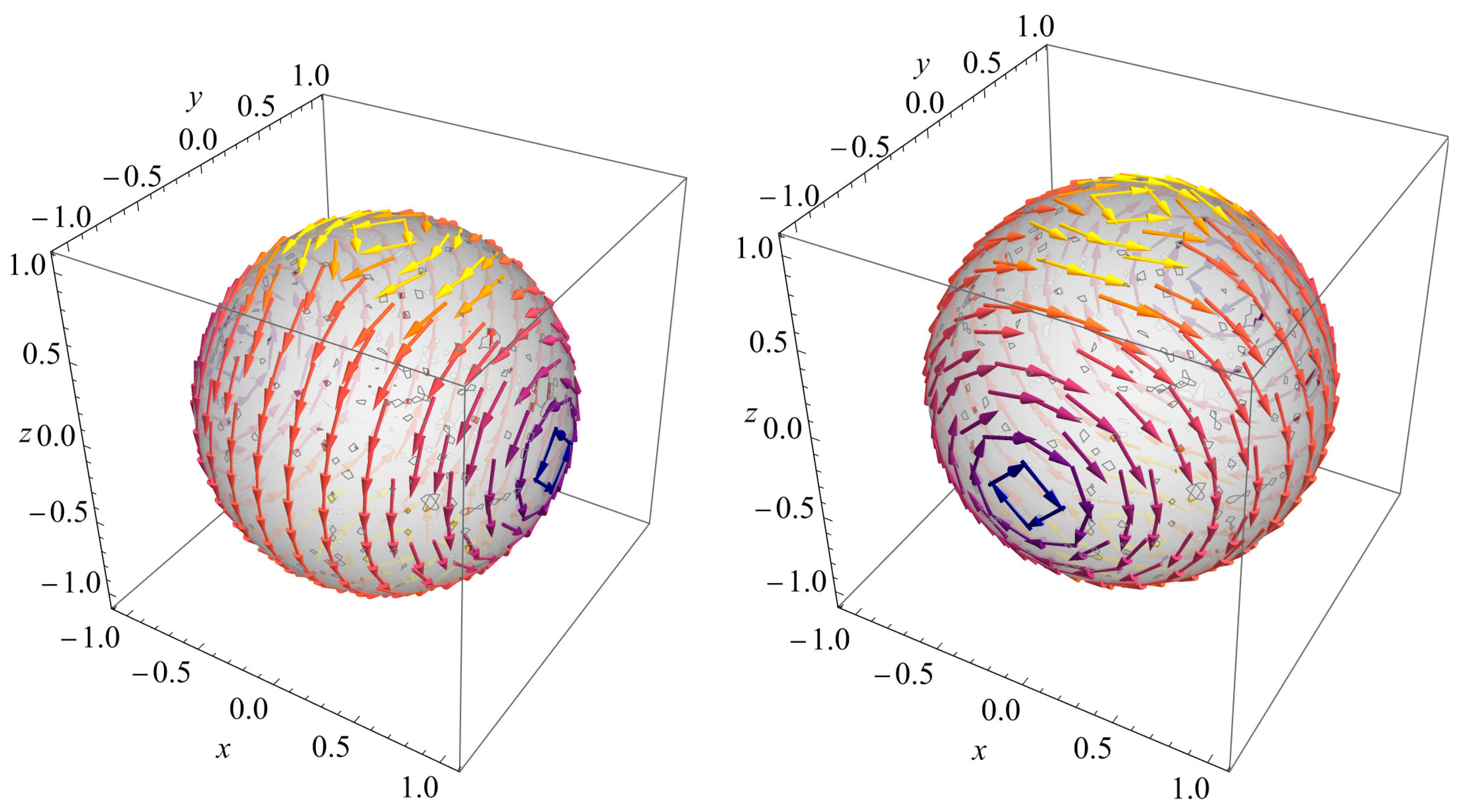
where the superscripts $1,2,3$ denote color indices. The current $\overrightarrow{j^3}$ has only the $\phi$ component; this means that this is a circular current creating a dipole with the color index 3. The currents $\overrightarrow{j^{1,2}}$ are shown in Figure 1. It is seen that these currents also form dipoles; this suggests that the solution under consideration can be called a “dipole” solution, enclosed in quotation marks because it also contains a nonvanishing component of the color magnetic field $H_{\phi }^a$. Further note that for the gauge (4) and spinor (5) fields, the zeroth component of the current $j^{a0}$ is equal to zero; this implies that, in our case, there is no source of a color electric field.

The total energy density of the “dipole” under consideration is

$$\widetilde{ϵ}={\widetilde{ϵ}}_m+{\widetilde{ϵ}}_s=\frac{1}{{\tilde{g}}_{\mathsf{\Lambda }}^2}\left[\frac{{f^{\prime }}^2}{x^2}+\frac{{\left(f^2-1\right)}^2}{2x^4}\right]+\left[\tilde{E}\frac{{\tilde{u}}^2+{\tilde{v}}^2}{x^2}+\frac{{\left({\tilde{u}}^2-{\tilde{v}}^2\right)}^2}{2x^4}\right].$$

(9)

Here the expressions in the square brackets correspond to the dimensionless energy densities of the non-Abelian gauge fields, ${\widetilde{ϵ}}_m\equiv \frac{{\left(l_0{\lambda }_c\right)}^2}{\hslash c}{ϵ}_m$, and of the spinor field, ${\widetilde{ϵ}}_s\equiv \frac{{\left(l_0{\lambda }_c\right)}^2}{\hslash c}{ϵ}_s$.

Correspondingly, the total energy of the “dipole” is calculated as

$${\tilde{W}}_t\equiv \frac{m_f{l}_0^2}{{\hslash }^2}{W}_t=4\pi \underset{0}{\overset{\infty }{\int }}{x}^2\widetilde{ϵ}dx={\left({\tilde{W}}_t\right)}_m+{\left({\tilde{W}}_t\right)}_s,$$

(10)

where the energy density $\widetilde{ϵ}$ is taken from Equation (9). In the right-hand side of Equation (10), the first term is the energy of the magnetic field and the second term corresponds to the energy of the nonlinear spinor field.

The typical behavior of ${\tilde{W}}_t$ as a function of the spinor frequency $\tilde{E}$ is sketched in Figure 2. It is seen that there exists an absolute minimum of the dimensionless energy (mass gap); call it $\tilde{\Delta }\left(g_{\mathsf{\Lambda }}^2\right)$. Moreover, as demonstrated in [7,8], for $\tilde{E}\to 0,1$, the energy of the “dipole” goes to infinity.

The asymptotic behavior of the functions $f,\tilde{v}$, and $\tilde{u}$ is as follows:

$$\begin{array}{cc}\hfill f\left(x\right)\approx & 1-\frac{f_{\infty }}{x},\hfill \end{array}$$

(11)

$$\begin{array}{cc}\hfill \tilde{u}\left(x\right)\approx & {\tilde{u}}_{\infty }{e}^{-x\sqrt{1-{\tilde{E}}^2}},\tilde{v}\left(x\right)\approx {\tilde{v}}_{\infty }{e}^{-x\sqrt{1-{\tilde{E}}^2}},\hfill \end{array}$$

(12)

where $f_{\infty },{\tilde{u}}_{\infty }$, and ${\tilde{v}}_{\infty }$ are integration constants.

Consider the question of a linear size of the “dipole” under investigation. It consists of two fields—the non-Abelian field $A_{\mu }^a$ and the spinor field $\psi$—whose asymptotic behavior is fundamentally different. As follows from Equation (11), the color field decreases according to the power law, $H_{r,\theta ,\phi }^a\sim r^{-3}$ [7], whereas the spinor field decreases exponentially with distance according to Equation (12). In this connection, it is difficult to introduce the notion of the size of the “dipole”. However, one may introduce the notion of the core of the “dipole”, which represents the region where the spinor field (which is a source of the color Yang–Mills field) is concentrated. Then, in accordance with Equation (12), one may define a characteristic size of the core of the “dipole” as

$$l_{cr}\approx \frac{{\lambda }_c}{\sqrt{1-{\tilde{E}}^2}}.$$

(13)

This implies that for $\tilde{E}\to 1$, the size of the core $l_{cr}\to \infty$. In turn, for $\tilde{E}\to 0$, it is estimated as $l_{cr}\approx {\lambda }_c$, i.e., it remains unchanged. Unfortunately, the power-law asymptotic behavior of the magnetic field (11) does not permit one to define a quantity that adequately represents the size of the “dipole” itself and not just the size of the core.

Taking into account that the linear size of the core is estimated according to Expression (13), a maximal number of DLFCs (“dipoles”) per unit volume can be estimated as

$${\left[n_{\mathrm{DLFC}}\left(\tilde{E}\right)\right]}_{\max }\approx {\left[l_{cr}\left(\tilde{E}\right)\right]}^{-3}.$$

Perhaps such concentration of the DLFCs is not attainable in vacuum, but it may be reached in a quark–gluon plasma at high temperatures.

3. “Dipoles” in Nonperturbative Vacuum

In this section, we describe a scenario within which “dipoles” found in [7,8] may be regarded as DLFCs in the nonperturbative vacuum of SU(2) Yang–Mills theory coupled to a nonlinear spinor field.

The main idea is the same as that used in Abelian magnetic monopole dominance: among all possible fluctuations of a gauge field, there are some that satisfy Equations (6)–(8). Thus, we suppose that, within the nonperturbative vacuum model under consideration, such configurations give the dominant contribution to the path integral in the theory with the Lagrangian (1). Since we consider vacuum, the mean vacuum values of all color potentials and of the spinor field are zero,

$$〈{\widehat{A}}_{\mu }^a〉=0,〈\widehat{\psi }〉=0,$$

whereas the dispersions of these fields are nonvanishing,

$$〈{\left({\widehat{A}}_{\mu }^a\right)}^2〉\ne 0,〈{\left(\widehat{\psi }\right)}^2〉\ne 0.$$

In the nonperturbative vacuum model under consideration, the dominant contribution to the nonvanishing magnitudes of the dispersions, as well as to higher-order Green’s functions, is given by DLFCs, whose averaged spatial distribution is sketched in Figure 3.

The system under consideration contains two parameters, ${\lambda }_c$ and $l_0$, having dimensions of length. The first determines the size of the core of the “dipole” created by the spinor field, and the second is the spinor field self-coupling constant, which characterizes the distance between DLFCs (see Figure 3). Thus, the theory contains two constants with the dimensions of length that determine the properties of the nonperturbative vacuum: the size of the core of DLFCs and the distance between them.

Let $n_{\mathrm{DLFC}}\left(\tilde{E}\right)$ be the average density of DLFCs per unit volume, which depends on the spinor frequency $\tilde{E}$; then, the average energy density of the nonperturbative vacuum can be defined as

$${\epsilon }_0\approx \frac{{\hslash }^2}{m_f{l}_0^2}〈n_{\mathrm{DLFC}}\left(\tilde{E}\right){\tilde{W}}_t\left(\tilde{E}\right)〉,$$

(14)

where the dimensionless energy ${\tilde{W}}_t$ is given by theExpression (10) and $〈\cdots 〉$ denotes the quantum averaging over all possible values of $\tilde{E}$.

The lifetime of a virtual DLFC with energy $W_t\left(\tilde{E}\right)$ is determined according to the Heisenberg uncertainty principle,

$$\Delta t\approx \frac{\hslash }{W_t\left(\tilde{E}\right)}=\frac{m_f{l}_0^2}{\hslash }\frac{1}{{\tilde{W}}_t\left(\tilde{E}\right)}.$$

(15)

This expression implies that the maximum lifetime is for a DLFC with energy equal to the energy of the mass gap ${\tilde{W}}_t\left(\tilde{E}\right)=\tilde{\Delta }\left(g_{\mathsf{\Lambda }}^2\right)$.

Consider next the behavior of the concentration of DLFCs $n_{\mathrm{DLFC}}\left(\tilde{E}\right)$ for $\tilde{E}\to 0,1$. For $\tilde{E}\to 1$, according to Equation (13), the linear size of the region occupied by the core of the “dipole” created by the spinor field approaches infinity, $l_{cr}\to \infty$. This actually means that the size of a DLFC approaches infinity as well; that is, one DLFC occupies all the space. This, in turn, means that

$$n_{\mathrm{DLFC}}\left(\tilde{E}\to 1\right)\to 0.$$

(16)

As we pointed out above, for $\tilde{E}\to 0$, the size of the core is estimated as $l_{cr}\approx {\lambda }_c$, whereas the value of the non-Abelian magnetic field goes to infinity and the field fills all the space. As in the case with $\tilde{E}\to 1$, this means that

$$n_{\mathrm{DLFC}}\left(\tilde{E}\to 0\right)\to 0.$$

(17)

Both Conditions (16) and (17) can be written as

$$n_{\mathrm{DLFC}}\left(\tilde{E}\right)\to 0\mathrm{when}\tilde{E}\to 0,1\mathrm{or},\mathrm{equivalently},\mathrm{when}{\tilde{W}}_t\left(\tilde{E}\right)\to \infty .$$

(18)

Thus, the function $n_{\mathrm{DLFC}}\left(\tilde{E}\right)$ is equal to zero at the boundaries of the interval $0⩽\tilde{E}⩽1$; this suggests that for some ${\tilde{E}}_0$ lying in this interval, the concentration $n_{\mathrm{DLFC}}\left({\tilde{E}}_0\right)$ has a maximum.

The expression for the energy density (14) is the product of two functions: the density of DLFCs and the dimensionless energy of a DLFC. For $\tilde{E}\to 0,1$, the first function, according to Equation (18), goes to zero, whereas the second one—to infinity. Consequently, their product in Equation (14) goes either to zero, or to a constant, or to infinity. In order for the energy density to be finite, it is necessary to choose the first option. This permits one to estimate the quantity (14) as the product of the characteristic value of the density of DLFCs $n_{\mathrm{DLFC}}\left({\tilde{E}}_0\right)$ and the characteristic value of the energy—the mass gap $\tilde{\Delta }\left(g_{\mathsf{\Lambda }}^2\right)$:

$${\epsilon }_0\approx \frac{{\hslash }^2}{m_f{l}_0^2}{n}_{\mathrm{DLFC}}\left({\tilde{E}}_0\right)\tilde{\Delta }\left(g_{\mathsf{\Lambda }}^2\right).$$

(19)

This expression indicates that, in the model under consideration, the energy density of nonperturbative vacuum ${\epsilon }_0$ is a finite quantity, in contrast to the energy of perturbative vacuum, which is infinite. Notice that in these calculations, the presence of a mass gap plays a crucial role. In the absence of the mass gap, the computation procedure is changed considerably and Expression (19) would already be incorrect.

One of the undetermined quantities in Expression (19) is the concentration of DLFCs $n_{\mathrm{DLFC}}\left({\tilde{E}}_0\right)$ with dimensions ${\left(\mathrm{length}\right)}^{-3}$. In the initial Equations (2) and (3), there are two quantities with dimensions of length: the Compton wavelength ${\lambda }_c$ and the spinor field coupling constant $l_0$. Therefore, one can assume that, in order of magnitude, the concentration might be estimated as

$$n_{\mathrm{DLFC}}\left({\tilde{E}}_0\right)\approx \frac{1}{l_0^{3-\alpha }{\lambda }_c^{\alpha }}.$$

(20)

The quantity ${\left(l_0^{3-\alpha }{\lambda }_c^{\alpha }\right)}^{1/3}$ characterizes the distance between DLFCs. The simplest case of $\alpha =0$ is sketched in Figure 3.

It is of interest to estimate characteristic quantities of the nonperturbative vacuum under consideration. To do so, we start from the assumption that its energy density (19) is of the order of the energy density associated with Einstein’s cosmological constant ${\mathsf{\Lambda }}_E$, i.e., ${\epsilon }_0={\epsilon }_{{\mathsf{\Lambda }}_E}\approx 5.4\times {10}^{-9}\mathrm{erg}{\mathrm{cm}}^{-3}$. As an example, take the following set of parameters: (i) let $\alpha =0$ in Equation (20); (ii) choose $m_f$ equal to, say, the mass of the strange quark $m_s\approx 95\mathrm{MeV}$; (iii) take the magnitude of the dimensionless mass gap to be $\tilde{\Delta }\left(g_{\mathsf{\Lambda }}^2\right)\approx 50$ [8]; and (iv) let ${g^{\prime }}^2\approx 10$ (typical value in QCD). Then, we have the following estimates:

$$\begin{array}{cc}\hfill & {\tilde{g}}_{\mathsf{\Lambda }}^2\approx 2.09\times {10}^{-17},\Delta \left(g_{\mathsf{\Lambda }}^2\right)\approx 1.59\times {10}^{-20}\mathrm{erg},m_{\Delta }\equiv \Delta \left(g_{\mathsf{\Lambda }}^2\right)/c^2\approx 1.77\times {10}^{-41}\mathrm{g},\hfill \\ \hfill & {\lambda }_c\approx 2.08\times {10}^{-13}\mathrm{cm},l_0\approx 1.44\times {10}^{-4}\mathrm{cm},n_{\mathrm{DLFC}}\approx 3.38\times {10}^{11}{\mathrm{cm}}^{-3}.\hfill \end{array}$$

(21)

For some reason, this does not allow us to regard the energy density of the nonperturbative vacuum as that associated with Einstein’s cosmological constant. One of these reasons is that the equation of state corresponding to the cosmological constant is $p_{{\mathsf{\Lambda }}_E}=-{\epsilon }_{{\mathsf{\Lambda }}_E}.$ The determination of the pressure of the nonperturbative vacuum (or its equation of state) is a challenging problem, and we will not address it here. The point is that the virtual DLFCs under consideration are extended objects, and for this reason, the following problems occur: (a) it is, in particular, unclear how they interact with a reflecting wall; (b) since the DLFCs under consideration are field objects, in order to consider their interactions, it is necessary to take into account corrections to the corresponding solutions; and (c) if the DLFCs are packed so closely that they begin to “touch” each other, then instead of a gas of DLFCs, there occurs some extended and continuous substance; this should be taken into account when performing calculations.

4. Discussion and Conclusions

In the present paper, we suggested a speculative model of nonperturbative vacuum in SU(2) Yang–Mills theory coupled to a nonlinear spinor field. Within this model, by analogy with Abelian magnetic monopole dominance, it is assumed that the main contribution to the energy of the nonperturbative vacuum comes from DLFCs, which are represented here by “dipoles” constructed in [7,8]. The remarkable feature of such nonperturbative vacuum is that its energy density is finite.

We summarize the results:

• The model of nonperturbative vacuum in SU(2) Yang–Mills theory coupled to a nonlinear spinor field is suggested, assuming that the main contribution to its characteristics comes from DLFCs that are described by the corresponding “dipole” solutions.
• We present arguments to claim that the number density of DLFCs whose energy approaches infinity goes to zero.
• We derive the expression for the energy density of the nonperturbative vacuum, which, being a sum of energies of DLFCs, is finite.
• Starting from the assumption that the magnitude of the nonperturbative vacuum energy density is of the order of the energy density associated with Einstein’s cosmological constant, we estimate the characteristic quantities of the nonperturbative vacuum under consideration.
• We suggest the physical interpretation of the spinor field self-coupling constant, having dimensions of length, as a quantity characterizing the distance between DLFCs in the nonperturbative vacuum.

We have pointed out that, although the energy density of the nonperturbative vacuum may be of the order of that associated with Einstein’s cosmological constant, for some reason it is difficult to identify these two quantities. For example, for the cosmological constant, it is necessary to have a strictly defined relationship between its energy density and pressure. In further studies on this subject, it will be necessary to determine an expression for the pressure of the nonperturbative vacuum, which amounts to obtaining an equation of state for such a vacuum. The principle problem one faces here is that the DLFCs are (i) quantum and virtual and (ii) extended objects.

Notice that the SU(2) Yang–Mills theory coupled to a nonlinear spinor field under consideration is a non-QCD theory. The principle difference is that in QCD, a spinor field is described by the linear Dirac equation, while here we deal with the nonlinear Dirac equation. At first glance, the linear and nonlinear Dirac equations are in no way related to each other. However, it is worth mentioning here that there is a possibility of obtaining the nonlinear Dirac equation as a consequence of nonpertubative quantization in QCD, as discussed in [7,8,19].

In conclusion, we wish to note that the model of nonperturbative vacuum under consideration is an experimentally testable model, at least in principle. The lifetime of a virtual DLFC is determined by Equation (15); then, e.g., for the parameters used in obtaining the estimates (21), one has $\Delta t\approx 6.6\times {10}^{-8}$ s. In turn, one cubic centimeter contains only ∼${10}^{11}$ virtual DLFCs. Since this concentration and the lifetimes are quite large quantities, one may expect that experimental verification of the existence of such virtual DLFCs might be possible.

Two other characteristics of nonperturbative vacuum in the model considered here are the parameters ${\lambda }_c$ and $l_0$ with dimensions of length. The first one determines the size of a charge created by the spinor field, and the second one is the self-coupling constant of the nonlinear spinor field, which, as we assumed above, characterizes the distance between DLFCs. Thus, in the present model of the nonpertubative vacuum, there are two constants with dimensions of length that determine the properties of the nonpertubative vacuum: the size of the central part of a DLFC and the distance between them. To test the model, these parameters may, in principle, be experimentally measured as well.

In conclusion, we would like to note that the nonperturbative vacuum is a very complex object, and its properties can differ in principle from the properties of perturbative vacuums, which are described in detail in standard textbooks on quantum field theory. Here, we suggested an approximate model of nonperturbative vacuum based on the existence of DLFCs populating such a vacuum. However, there may exist field theories in which such particle-like solutions are absent. In that case, an investigation of the properties of nonperturbative vacuum becomes even more complicated. One might expect that this can be done using an infinite set of differential Schwinger–Dyson equations written in a nonperturbative form (as done, for example, in [19]). Such a set of equations should describe both excited states and a vacuum.

References

- Kondo, K.I. Abelian magnetic monopole dominance in quark confinement. Phys. Rev. D 1998, 58, 105016. [Google Scholar] [CrossRef] [Green Version]
- Suzuki, T.; Yotsuyanagi, I. A possible evidence for Abelian dominance in quark confinement. Phys. Rev. D 1990, 42, 4257. [Google Scholar] [CrossRef] [PubMed]
- Ezawa, Z.F.; Iwazaki, A. Abelian Dominance and Quark Confinement in Yang-Mills Theories. Phys. Rev. D 1982, 25, 2681. [Google Scholar] [CrossRef]
- Ezawa, Z.F.; Iwazaki, A. Abelian Dominance and Quark Confinement in Yang-Mills Theories. 2. Oblique Confinement and η′ Mass. Phys. Rev. D 1982, 26, 631. [Google Scholar] [CrossRef]
- Arasaki, N.; Ejiri, S.; Kitahara, S.i.; Matsubara, Y.; Suzuki, T. Monopole action and monopole condensation in SU(3) lattice QCD. Phys. Lett. B 1997, 395, 275. [Google Scholar] [CrossRef] [Green Version]
- Chernodub, M.N.; Polikarpov, M.I. Abelian projections and monopoles, Contribution to: NATO Advanced Study Institute on Confinement, Duality and Nonperturbative Aspects of QCD. arXiv 1997, arXiv:hep-th/9710205. [Google Scholar]
- Dzhunushaliev, V.; Folomeev, V.; Serikbolova, A. Monopole solutions in SU(2) Yang-Mills-plus-massive-nonlinear-spinor-field theory. Phys. Lett. B 2020, 806, 135480. [Google Scholar] [CrossRef]
- Dzhunushaliev, V.; Burtebayev, N.; Folomeev, V.N.; Kunz, J.; Serikbolova, A.; Tlemisov, A. Mass gap for a monopole interacting with a nonlinear spinor field. Phys. Rev. D 2021, 104, 056010. [Google Scholar] [CrossRef]
- ’t Hooft, G. Magnetic Monopoles in Unified Gauge Theories. Nucl. Phys. B 1974, 79, 276. [Google Scholar] [CrossRef] [Green Version]
- Polyakov, A.M. Particle Spectrum in Quantum Field Theory. JETP Lett. 1974, 20, 194. [Google Scholar]
- Li, X.Z.; Wang, K.l.; Zhang, J.Z. Light Spinor Monopole. Nuovo Cim. A 1983, 75, 87. [Google Scholar]
- Wang, K.L.; Zhang, J.Z. The Problem of Existence for the Fermion-Dyon Selfconsistent Coupling System in a SU(2) Gauge Model. Nuovo Cim. A 1985, 86, 32. [Google Scholar]
- Finkelstein, R.; LeLevier, R.; Ruderman, M. Nonlinear Spinor Fields. Phys. Rev. 1951, 83, 326. [Google Scholar] [CrossRef]
- Finkelstein, R.; Fronsdal, C.; Kaus, P. Nonlinear Spinor Field. Phys. Rev. 1956, 103, 1571. [Google Scholar] [CrossRef]
- Belavin, A.A.; Polyakov, A.M.; Schwartz, A.S.; Tyupkin, Y.S. Pseudoparticle Solutions of the Yang-Mills Equations. Phys. Lett. B 1975, 59, 85. [Google Scholar] [CrossRef]
- Harrington, B.J.; Shepard, H.K. Periodic Euclidean Solutions and the Finite Temperature Yang-Mills Gas. Phys. Rev. D 1978, 17, 2122. [Google Scholar] [CrossRef]
- Lee, K.M.; Lu, C.H. SU(2) calorons and magnetic monopoles. Phys. Rev. D 1998, 58, 025011. [Google Scholar] [CrossRef] [Green Version]
- Prasad, M.K.; Sommerfield, C.M. An Exact Classical Solution for the ’t Hooft Monopole and the Julia-Zee Dyon. Phys. Rev. Lett. 1975, 35, 760. [Google Scholar] [CrossRef]
- Dzhunushaliev, V.; Folomeev, V. QCD Effects in Non-QCD Theories. Found. Phys. 2022, 52, 118. [Google Scholar] [CrossRef]
Figure 1.
Sketches of the force lines of the components of the color current (left panel) and (right panel) on the surface . The plots are given in Cartesian coordinates .
Figure 2.
A sketch of the energy spectrum of the total energy from Equation (10) as a function of the spinor frequency (for details, see [7]).
Figure 3.
A sketch of the averaged spatial distribution of DLFCs in the nonperturbative vacuum; their location in space is randomly changed, and this leads to nonzero values of the dispersions and of higher-order Green’s functions. The size of the core is characterized by the Compton wavelength of a fermion with mass (cf. Equation (13)). The average distance between DLFCs is determined by the spinor field self-coupling constant .
Publisher’s Note: MDPI stays neutral with regard to jurisdictional claims in published maps and institutional affiliations. |
© 2022 by the authors. Licensee MDPI, Basel, Switzerland. This article is an open access article distributed under the terms and conditions of the Creative Commons Attribution (CC BY) license (https://creativecommons.org/licenses/by/4.0/).
Share and Cite
MDPI and ACS Style
Dzhunushaliev, V.; Folomeev, V. Dipole-like Field Configurations in Nonperturbative Vacuum. Symmetry 2022, 14, 2659. https://doi.org/10.3390/sym14122659
AMA Style
Dzhunushaliev V, Folomeev V. Dipole-like Field Configurations in Nonperturbative Vacuum. Symmetry. 2022; 14(12):2659. https://doi.org/10.3390/sym14122659
Chicago/Turabian StyleDzhunushaliev, Vladimir, and Vladimir Folomeev. 2022. "Dipole-like Field Configurations in Nonperturbative Vacuum" Symmetry 14, no. 12: 2659. https://doi.org/10.3390/sym14122659
Note that from the first issue of 2016, this journal uses article numbers instead of page numbers. See further details here.