
On a Novel Dynamics of SEIR Epidemic Models with a Potential Application to COVID-19


1
Department of Mathematics, Sri Eshwar College of Engineering, Coimbatore 641 202, Tamilnadu, India
2
Department of Mathematics, Université de Caen Basse-Normandie, F-14032 Caen, France
3
Faculty of Natural Sciences and Mathematics, Escuela Superior Politécnica del Litoral ESPOL, Guayaquil 090902, Ecuador
4
Faculty of Engineering, Universidad Espíritu Santo, Samborondón 0901952, Ecuador
5
School of Industrial Engineering, Pontificia Universidad Católica de Valparaíso, Valparaíso 2362807, Chile
*
Author to whom correspondence should be addressed.
Symmetry 2022, 14(7), 1436; https://doi.org/10.3390/sym14071436
Submission received: 16 May 2022
/
Revised: 22 June 2022
/
Accepted: 5 July 2022
/
Published: 13 July 2022
Abstract
:In this paper, we study a type of disease that unknowingly spreads for a long time, but by default, spreads only to a minimal population. This disease is not usually fatal and often goes unnoticed. We propose and derive a novel epidemic mathematical model to describe such a disease, utilizing a fractional differential system under the Atangana–Baleanu–Caputo derivative. This model deals with the transmission between susceptible, exposed, infected, and recovered classes. After formulating the model, equilibrium points as well as stability and feasibility analyses are stated. Then, we present results concerning the existence of positivity in the solutions and a sensitivity analysis. Consequently, computational experiments are conducted and discussed via proper criteria. From our experimental results, we find that the loss and regain of immunity result in the gain and loss of infections. Epidemic models can be linked to symmetry and asymmetry from distinct points of view. By using our novel approach, much research may be expected in epidemiology and other areas, particularly concerning COVID-19, to state how immunity develops after being infected by this virus.
Keywords:
ABC derivatives; basic reproduction number; equilibrium points; fractional derivatives; Laplace transform; numerical methods; SARS-CoV-2; sensitivity and stability analysesMSC:
34A08; 65H10; 70-10; 92-101. Introduction
Epidemic models are widely applied and helpful to different purposes. Diverse types of epidemic models are available in the literature [1,2,3,4], such as susceptible, infected, recovered (SIR) and its variants: exposed (SEIR), SEIR-asymptomatic (SEIAR), vaccinated (SVIR), SEIAR-vaccinated (SEVIAR), SVIR-asymptomatic (SAVIR), with deceased (SIRD), cross-immunity component (SIRC), and with quarantine (SIRQ).
In [5,6,7], applications of these models to Latin America data concerning the severe acute respiratory syndrome coronavirus 2 (SARS-CoV-2), known as COVID-19 [8,9], were derived. The virus started in December 2019 in Wuhan, China, and was declared a pandemic in March 2020 by the World Health Organization (www.who.int: accessed 7 July 2022). COVID-19 has affected the world’s population and economy [10,11,12], forcing us to adopt a new life way forever. The COVID-19 epidemic can be formulated as non-linear mathematical models. To deal with these models for SARS-CoV-2, various tools have been introduced in the literature. In [13,14], modeling of the COVID-19 dynamics with fractional derivatives was carried out.
In [15], India’s lockdown for COVID-19 was investigated employing a SEIR model. In [16], solutions for COVID-19 in terms of stiff differential equations and fuzzy theory were provided. In [17], a SEIR model for forecasting and controlling COVID-19 outbreaks was presented. In [18], the influence of channel reporting on the COVID-19 outbreak was thoughtfully explained by using dynamical models to examine the interaction of the disease progression. In [19], a latent treatment of COVID-19 was predicted utilizing epidemic models.
In general, many other real phenomena, in addition to COVID-19, may be described by non-linear models, such as mentioned next. Although no mathematical models were presented in [20], influenza types A, B, and C were analyzed and found to be helpful in gaining some knowledge on disease spread. In [21], a Newton algorithm for the Adomian decomposition method (ADM) was proposed. In [22], fractional differential equations (FDEs) and Schrodinger equations were evaluated. In [23], the ADM approach to an SIR model was considered and analyzed. In [24], the Nagumo uniqueness results for some real models were reviewed. In [25], Riemann–Liouville integrals of non-discrete bounded variations were studied. In [26], a vaccination model of diseases affecting infants was applied. In [27], a fractional SIRC model for type A influenza was formulated. In [28], a kernel application for heat transfer was developed for a Lyapunov type inequality. In [29], solutions to the measles problem utilizing the Laplace ADM (LADM) were proposed. In [30], efficient prevention of cancer was studied. In [31], a SIR model was presented employing fractional operators with a non-singular Mittag–Leffler kernel [32]. In [33], non-linear equations were performed with global operators and applied to epidemiology. In [34], fractional differential products were defined. In [35], the LADM for the human immunodeficiency of differentiation 4 with T helper cells, CD4T in short, was applied. In [36,37], a SIRD model with and without delay was presented. In [38], the stability of the Riemann–Liouville differential system was presented. In [39], dengue transmission with a preventive formula was presented [40]. In [41], SEIQ model dynamics were introduced. In [42], a way to solve boundary-value problems for Riemann–Liouville fractional derivatives was obtained. In [43], initial value problems for Riemann–Liouville sequential derivatives were solved. In [44], dengue transmission derivatives were estimated. In [45], the stability of a SIR model with vaccination was stated.
As mentioned, epidemic models can be linked to symmetry and asymmetry from different points of view such as: patchy epidemic environments, itinerant population exchange matrices, epidemic models describing networks, and time-invariant epidemic model parameterizations, among others; see details in [46] and references therein.
Note that the transmission dynamics of a viral infection are as follows. First, when there is a contact between a susceptible and an infected person, there is a probability that transmission occurs, and then the susceptible person enters the exposed class in the latent period, who are infected but not yet infectious. Second, after the latent period ends, the exposed individual enters the infected class, who are infectious in the sense that they can transmit the infection. Third, when the infectious period ends, the infected individual enters the recovered class consisting of those with permanent or transient infection-acquired immunity.
One can consider both exposed (infected but not infectious) and infected people (who are also infectious) as recovered. A point here is whether people who are infected but not yet infectious (exposed) will be able to recover only after transmitting infections to others. In mathematical modeling, one avoids simultaneous changes in the system. However, in biology, simultaneous changes will occur as exposed and infected people recover. Therefore, one can create a new model that behaves according to simultaneous changes. Moreover, if all the exposed individuals must be recovered only after becoming infectious, then the meaning of the basic reproduction number will fail because there will be further waves, and it sounds like recovery should be there only after infecting others. A novel idea that can be proposed is that the exposed rate may be very low, but the infected and other rates may be significant.
Based on the bibliographical review presented above, to the best of our knowledge, epidemic models describing diseases that unknowingly spread for a long time, but by default spread only to a minimal population, including the novel ideas stated above, have not been proposed until now.
The main objective of our investigation is to introduce a new variation of the SEIR epidemic model, which deals with the transmission between susceptible, exposed, infected, and recovered classes in the manner established above. The novel variation of the SEIR epidemic model, proposed in the present work, uses a fractional differential system under the Atangana–Baleanu–Caputo (ABC) derivative.
After formulating the model as ordinary differential equations (ODEs), we transform it into an ordered model by employing FDEs. We also analyze the basic reproduction number, stability, and numerical simulations, as developed in [29,47]. Another new idea presented in this investigation is in the stability analysis, where we considered the initial populations as well as disease-free and disease-dependent equilibrium points. The stability of the system depends on whether the initial points of the system converge when the system is subject to no change. In addition, we examine whether the equilibrium points, instead of initial values, converge to equilibrium points or not. From our experimental results, we find that the loss and regain of immunity result in the gain and loss of infections. Evidently, applications to COVID-19 can be potentially attractive. Indeed, it would be interesting to state how immunity develops after being infected by SARS-CoV-2, which presents a potential application of our results.
The structure of this new work is arranged as follows. The formulation of the model is stated in Section 2. In this section, necessary preliminary knowledge is also introduced. In Section 3, we provide equilibrium values and stability, as well as a feasibility analysis. Section 4 includes a sensitivity analysis and the retention of positive bounds of solutions. Our numerical experimental results are reported in Section 5. Finally, the conclusions of the present study are sketched in Section 6.
2. Background
In this section, we first present the SEIR model. Then, some important known results on FDEs under the ABC derivative principles are provided.
2.1. SEIR Epidemic Model
To formulate our epidemic mathematical model, consider the equations stated as
where the functions , , , and in the SEIR model defined in (1) allow us to calculate the number of susceptible, exposed, infected, and recovered people at time t, respectively. In addition, the constants a, b, c, and r represent the rates at which susceptible become exposed, the exposed become infected, the exposed become recovered, and the infected become recovered, respectively. Note that
where stated in (2) is the total population at time t. Note that is not constant because of births and deaths, or at least few who are not even susceptible at the considered time.
To determinate the SEIR model formulated in (1), we must consider , , , , and , which represent the initial values of the corresponding populations. Figure 1 illustrates all the model variables and their interactions. Some notations used in our work are summarized in Table 1, where we can also see the initial data and values of the rates to be used in the simulations carried out in this investigation. We take such values to make the system stable and positively bounded. Note all the values satisfy the model. Some works [16,36,37] have considered nearby values. With these values, we can introduce a new variation of the SEIR epidemic model, which deals with the transmission between susceptible, exposed, infected, and recovered classes.
2.2. Contextualization of the New Epidemic Model
We have provided the mathematical background of the model. However, some aspects that arise when formulating the model need to be discussed. For example, the model sometimes seems not to describe a real viral infection. This is because both the model equation and the corresponding fractional equation show that the exposed population is infected but not infectious, making it necessary to move the symptomatic or asymptomatic cases to the compartment of the infected population. Furthermore, because the immune response to viral infections is not included in Figure 1, as well as the incubation period to attain the infection from being exposed with symptoms, the question of how an exposed case directly moves on to the recovered compartment may arise.
The answer to this question is that, to formulate the standard SEIR model in four compartments and not omit any features of asymptomatic and symptomatic behavior, we must consider both in the exposed population. However, we develop the model to analyze the rate of infectious people recovering and the rate of exposed people recovering. Initially, we planned to develop this model with an incubation period. Nevertheless, as our idea is to build an ODE model, based on existing models with an incubation period and an immune response, we did not openly disclose the immune response and incubation period (as we must include the delay term) when developing this model.
The immune response parameter may be added when the vaccination is adopted (that is, an SVIR model). Nonetheless, for our model, depending on individual immunity, some exposed individuals recovered even without treatment or vaccination. This is what we try to explain via our model. However, in the future, our model can be developed into SAVIR or SEIAR models using delay differential equations. For these equations, we must include the delay term as the incubation period and the immune response since the vaccination strategy plays a significant role. Moreover, our motivation is to build a four-compartment SEIR model that exhibits the properties of a five-compartment SEIAR model, as mentioned.
In the image of Figure 1, some exposed cases are moving to the recovered population because not all the people who are being exposed are also infected, but they might not be aware of their infection. They might also be asymptomatic, with the asymptomatic being hidden since we want to create and analyze such four-to-five compartments. This is because we assume that exposed individuals who are infected but not infectious (latent individuals) may move to the compartment of infected individuals (symptomatic or asymptomatic). Then, we bring them directly to the recovered compartment. We try to say that not all those exposed are infected but infectious, although they are exposed, even if they are unaware of their infection and have not been clinically diagnosed to be infected.
As mentioned, to the best of our knowledge, the description of the disease above presented is a new formulation. We have also discussed this with some experts, who say asymptomatic or symptomatic conditions are common in infected populations. Nevertheless, exposure is different depending upon the test, the clinics that perform tests, the equipment used to perform tests, and the time of performing tests. The results may vary because some exposed individuals are found to be infected, but not all exposed people are found to be infected, or even asymptomatic despite being infected. In such circumstances, there is a high probability for any exposed person to recover naturally, which supports the formulation of our model.
2.3. Preliminaries on Fractional Differential Equations
Next, a few important known results for FDEs considering the ABC derivative principles are provided. The rate of changes in epidemic models is very small, occurring in less than a unit of time. This negligible quantity of small changes can be studied only using FDEs and not ODEs. Thus, it is recommended to study the epidemic models in fractional derivative systems of equations rather than under ordinary systems. In addition, the fractional order models have one more degree of freedom than the ordinary integer order model when fitting data.
Biomedically, an oscillatory time series of infected cases might be sought. One would expect that the fractional model yields fractal curves with different scaling properties of the classical SEIR model. However, note that our model is stable after the first wave, so that we cannot obtain oscillatory curves. Oscillations occur on multiple waves and on sudden disturbances and bifurcations, among other aspects. If we add an incubation period as a delay term, then there would be a high chance of obtaining both oscillatory and fractal curves. Next, we define the ABC derivative, its Laplace transform, and the Atangana–Balenanu integral.
Definition 1
Definition 2
([28]). The Laplace transform of the ABC derivative of Definition 1 is given by
where is the Laplace transform of .
Definition 3
3. Mathematical Analysis
In this section, we provide equilibrium values, and stability and feasibility analyses.
3.1. Basic Reproduction Number
A key concept of the epidemic models is the basic reproduction number (), which is information that is helpful for establishing vaccination policies [5]. Observe that is the expected number of secondary (new) infected cases, produced by a primary infected case, for the full period of infectiousness (epidemic), when this infected case is introduced into a large population of susceptible cases. Hence, determination of facilitates proper vaccination policies. An epidemic may be initiated if ; otherwise, this can quickly end if . In summary, the basic reproduction number is a predictive calculation for stating how many new cases will occur from an infected individual.
At time , the rate of infection causes new susceptibilities. However, in our case, the exposure itself may make other individuals susceptible. Thus, instead of the population of infected people, we assume the exposed population at as
In addition, we have that
Furthermore, the threshold point or epidemic critical community size is given by
Note that, if , the disease recurs, that is, there is an epidemic. Otherwise, if , the disease does not spread. Based on the values of Table 1, we find that and . Since is less than one (even being almost at a minimum), the disease will not survive. Moreover, as and then , the disease will not recur, that is, there will not be an epidemic.
3.2. Equilibrium Points
In the expression given in (3), initial values stated as can be stated. Then, once again based on the fixed values of Table 1, from our calculations, the disease-free equilibrium points, that is, zero order derivatives, are , or , or . Note that the equilibrium points of disease dependance are obtained to be
and then
3.3. Feasibility Region Analysis
The following lemma considers the solution of the model to be restricted to a feasible region and then to detect when the epidemic outbreak will occur.
Lemma 1.
Let be the total population at t, and be the total population at . In addition, restrict the solution of the model under consideration to the feasible region defined as . Then, the epidemic outbreak will occur when .
Proof.
Let
Then, we obtain
Now, summing all the terms stated in (3), we obtain
Thus, we have
which means that
In a similar fashion, when , we have In the same way, we claim that and . Note that, if , then . Otherwise, if , then we have that , and . Thus, we verify that the decrease in infected cases will not lead to an epidemic outbreak, whereas an epidemic will occur when there is a drastic increase in infected cases due to susceptible cases. □
Theorem 1.
The system defined in (3) is asymptotically stable in a global way if it is asymptotically stable for:
- (i)
- The initial populations.
- (ii)
- All possible disease-free equilibrium points.
- (iii)
- The disease-dependent equilibrium points.
Proof.
Let the Jacobian matrix of the system presented in (3) be stated as
Then, the characteristic polynomial of the matrix defined in (4) is given by
Now, by grouping the terms of the polynomial defined in (5), we have that
Hence, fixing the values of a, b, c, and r as in Table 1 and using the formula defined in (6), we obtain that
Therefore, the real parts of the eigenvalues, that is, the zeros of the polynomial stated in (7), are given by
Figure 2 shows a plot with the real and imaginary parts of the eigenvalues obtained in (8) of the matrix stated in (4). Consequently, the system presented in (3), formed with the initial populations, is asymptotically stable since we find that only negative real parts in all the eigenvalues exist, with no imaginary parts being found.
Now, assume the Jacobian, formed of two disease-free equilibrium points, defined as
Observe that, when , the characteristic polynomial of the matrix established in (9) is presented as
As a result of fixing the values of a, b, c, and r as in Table 1 and using the formula stated in (10), we obtain
Therefore, the vector whose entries are the real parts of the eigenvectors of the polynomial formulated in (11) is expressed as
Figure 3 shows the real and imaginary parts of the eigenvalues given in (12) of the matrix stated in (9). Thus, the system presented in (3), formed by disease-free equilibrium points, is asymptotically stable because all eigenvalues have negative real parts.
In the case of the Jacobian matrix formed of two disease-free equilibrium points, its characteristic polynomial, when , is defined as
After fixing the values of a, b, c, and r as in Table 1 and utilizing the formula given in (13), we get
Therefore, the vector whose entries are the real parts of the eigenvectors of the polynomial formulated in (14) is expressed as
Figure 4 shows the real and imaginary parts of the eigenvalues given in (15), with no imaginary parts being found. Thus, the system presented in (3), formed by disease-free equilibrium points, is asymptotically stable because all its eigenvalues have negative real parts.
Next, consider the Jacobian matrix, with disease-dependent equilibrium points, defined by
Observe that, when , the characteristic polynomial of the matrix stated in (16) is given by
By considering the values of a, b, c, and r presented in Table 1 and the formula defined in (17), we reach
Hence, the vector whose entries are real parts of the eigenvectors of the polynomial expressed in (18) is given by
Figure 5 depicts the real and imaginary parts of the eigenvalues stated in (19), with no imaginary parts. Then, the system presented in (3) is asymptotically stable because all its eigenvalues have negative real parts.
Therefore, since all the conditions are satisfied, we can assert that the system defined in (3) is asymptotically stable in a global way, so that the result is proved. □
4. Positivity in Solutions and Sensitivity Analysis
In this section, first, we provide results on the existence of positivity in the solutions of the system. Then, we describe a sensitivity analysis.
4.1. Existence of Positivity in Solutions
The following theorem provides three important results.
Theorem 2.
Let be the total population at t and the initial total population. Then, the following results hold for all :
- (i)
- The solution of the SEIR model is positive for any non-negative initial conditions and for all t.
- (ii)
- The total population remains unvaried even for a long time, which holds for any given arbitrary non-negative initial conditions.
- (iii)
- All the solutions are positively bounded.
Proof.
After solving the ABC derivative system of order stated in (3), we obtain the solutions of as
where is often equal to zero. We know that the total population is equal to the sum of all cases, that is, . Moreover, from , we obtain
The obtained solution is , implying . Hence, the total population is positive for all . Then, proofs of (i) and (iii) are complete. Now, assume that . As , we have that , which implies that the population does not vary for all Thus, the global stability of the system is well established, proving (ii). The above proof shows the positive boundedness of , , , and , as noted in Figure 6 as well. □
4.2. Sensitivity Analysis
A sensitivity analysis is a tool to compare how each state variable influences the basic reproduction of the infection. This analysis is used to examine the effect of different parameters employed in the model on its output. Often sampled ranges of all the parameters utilizing statistical techniques are employed [48]. The formula used to compute the sensitivity index of a parameter x is given by
Now, the expression stated in (20), when applied to our model, based on the fixed values of Table 1 and from our calculations, allows us to obtain the values given by
Based on the values of the indices , , and presented in (21)–(23), respectively, we can conclude that the basic reproduction of secondary infection is primarily influenced by a, rather than b and r. When the sensitivity index of a increases or decreases by , will increase or decrease by the same , whereas b and r are less dominant in causing secondary infections. Figure 7 shows a plot with the three mentioned indices.
5. Numerical Results
In this section, we report the numerical results of our investigation.
5.1. Graphical Representation of , , , and
Figure 8 shows a block diagram performed with SIMULINK of Matlab, and executed with SOLVER of SIMULINK, using the fourth-order Runge–Kutta method. Note that this block diagram is a graphical representation of a first-order vector initial value problem. We consider the system given in (1), which is the vector initial value problem proposed by us.
The values obtained for , , , and , as a result of the computational experiments carried out, are plotted in Figure 9 for the considered differential system using , for all and . When executing the fourth-order Runge–Kutta method for our system given in (1), with 52 equally spaced approximation points between 0 and 1000, we obtain a numerical solution as presented in Figure 9. For the analytical solution of the SEIR model, the LADM method is used, which we describe next. From our experimental results, we find that the loss and regain of immunity result in the gain and loss of infections, which is described in Figure 9.
5.2. Laplace Adomian Decomposition Method
To solve our fractional SEIR epidemic model analytically, we use the LADM [29]. The functions , , , and are computed as
where stated in (24) is called the Adomian polynomial and is defined as
with , , and so on, with representing the inverse Laplace transform of . Now, we set
For the model formulated in (3), after collecting all the parametric values, the solution obtained by the LADM up to fourth order, that is, , is found as
Note that the solutions given in (25) are polynomials of fourth degree for the independent variable t with . We have omitted here the polynomials for the fractional case due to restrictions of space because their expressions are big. Plots of the number , , , and over time of the SEIR model are shown in Figure 10, for eleven solutions, each of them based on the th fractional derivative with , for all . The fractional derivatives were calculated with the Mathematica software.
6. Conclusions and Discussion
In this paper, we derived a novel SEIR epidemic model for describing diseases that unknowingly spread for a long time, but by default spread only to a minimal population. This new model deals with the transmission between susceptible, exposed, infected, and recovered classes. We considered both exposed (infected but not infectious) and infected people (who are also infectious) as recovered. A point that we considered is whether people infected but not yet infectious (exposed) will be able to recover only after infecting others. In mathematical modeling, one avoids simultaneous changes in the system. However, in biology, simultaneous changes will occur as exposed and infected people recover. We created a model that behaves according to simultaneous changes. Moreover, if all the exposed individuals must be recovered only after becoming infectious, the meaning of the basic reproduction number will fail because there will be further waves, and it sounds like recovery occur only after infecting others.
A novel idea that we proposed is that the exposed rate may be very small, but the infected and other rates may be significant. The model was expressed in terms of both ordinary and fractional differential equations, transforming the former into an ordered system under the Atangana–Baleanu–Caputo derivative. The solutions obtained from the Laplace Adomian decomposition were used to illustrate various orders of the Atangana–Baleanu–Caputo fractional differential system.
After formulating the model, equilibrium points as well as stability and feasibility analysis were stated. We examined whether the equilibrium points converge or not. In addition, we presented another new idea by means of a stability analysis, considering the initial populations and also both disease-free and disease-dependent equilibrium points. We reported that the stability of the system depends on the initial points of the system when converging to the equilibrium point, if the system is subject to no change. To provide the readers a visualization of how the real and imaginary parts of eigenvalues are used to reach the stability of the system, we gave several illustrations.
In addition to the stability analysis, feasibility region and sensitivity analysis were performed to demonstrate that the coefficient of the number of susceptible cases is dominant over the basic reproduction number. Depending on the initial populations and very slow spread of disease, we understand that this slow spread may increase the recovery rate by increasing immunity after infection. Complementary to the above-mentioned results, we established the existence of positivity in the solutions and show it graphically in Figure 6. Moreover, a sensitivity analysis was provided as displayed in Figure 7. Computational experiments were conducted employing proper criteria. From our experimental results, we found that the loss and regain of immunity resulted in the gain and loss of infections.
We introduced a new model that might behave simultaneously as susceptible, infected, and exposed (SER) and SEIR. The population is not constant because, for our model, when considering the SEIR (either both SER and SEIR; or only SEIR), certainly (net population since everyone is in the closed system) or only. From our results, we showed the model is stable and there were no bifurcations. Note that our model is biologically sensible to pass from the exposed class to the recovered class. Biologically, such simultaneous changes exist. However, in mathematical modeling, one does not consider them for convenience. In this work, we did not include immune response since we study how exposed and infected people recover from their natural immunity. If we assume an SVIR model, we should include immune response, as we are artificially trying to boost the immunity by providing the vaccinations.
Note that, in our study, we analyze only fractional ordinary differential equations. We hope to incorporate, in a future study, fractional delay differential equations into a SEVIAR model. It can be more convenient to use the incubation period in delay differential equations and immune response with vaccination strategy and people exposed to both asymptomatic and infected people may be incorporated. Furthermore, the impact of humoral and cell immunity responses upon the dynamics of the transmission of SARS-CoV-2 will be explored in a forthcoming study.
The incubation period is the sum of latent and infectious periods; that is, it is the time period in which someone acquires the infection until the onset of the disease. During the latent period (exposed class), the virus infects some cells of the body, and when there is what clinicians call “shedding of the virus”, the individual enters the infectious class.
By using our novel approach, much research can be initiated in epidemiological studies and in other fields. In particular, to confront the COVID-19 pandemic, we study how immunity can be developed after being infected by this virus. We hope to report potential findings in the future concerning these and other issues related to the present investigation.
Author Contributions
Conceptualization, M.R., C.C., C.M.-B., V.L.; data curation, M.R.; formal analysis, M.R., C.C., C.M.-B., V.L.; investigation, M.R., V.L.; methodology, M.R., C.C., C.M.-B., V.L.; validation, C.M.-B. and V.L.; writing—original draft, M.R., C.C.; writing—review and editing, C.M.-B., V.L. All authors have read and agreed to the published version of the manuscript.
Funding
This research was supported partially funded by FONDECYT grant number 1200525 (V.L.) from the National Agency for Research and Development (ANID) of the Chilean government under the Ministry of Science, Technology, Knowledge, and Innovation.
Institutional Review Board Statement
Not applicable.
Informed Consent Statement
Not applicable.
Data Availability Statement
Not applicable.
Acknowledgments
The authors would also like to thank three reviewers for their constructive comments which led to improvement in the presentation of the manuscript.
Conflicts of Interest
The authors declare no conflict of interest.
References
- Kermack, W.O.; Mckendrick, A.G. A contribution to the mathematical theory of epidemics. Proc. R. Soc. A 1927, 115, 700–721. [Google Scholar]
- Allen, L.J.S. An Introduction to Mathematical Biology; Prentice-Hall: New Jersey, NJ, USA, 2007. [Google Scholar]
- Fierro, R.; Leiva, V.; Balakrishnan, N. Statistical inference on a stochastic epidemic model. Commun. Stat. Simul. Comput. 2015, 44, 2297–2314. [Google Scholar] [CrossRef]
- Esquivel, M.L.; Krasii, N.P.; Guerreiro, G.R.; Patricio, P. The multi-compartment SI (RD) model with regime switching: An application to COVID-19 pandemic. Symmetry 2021, 13, 2427. [Google Scholar] [CrossRef]
- Jerez-Lillo, N.; Lagos-Alvarez, B.; Munoz-Gutierrez, J.; Figueroa-Zuniga, J.; Leiva, V. A statistical analysis for the epidemiological surveillance of COVID-19 in Chile. Signa Vitae 2022, 18, 19–30. [Google Scholar]
- Molin, R.M.H.D.; Gomes, D.S.R.; Cocco, M.V.; Santos, C.L.D. Short-term forecasting COVID-19 cumulative confirmed cases: Perspectives for Brazil. Chaos Solitons Fractals 2020, 135, 109853. [Google Scholar]
- Ospina, R.; Leite, A.; Ferraz, C.; Magalhaes, A.; Leiva, V. Data-driven tools for assessing and combating COVID-19 out-breaks based on analytics and statistical methods in Brazil. Signa Vitae 2022, 18, 18–32. [Google Scholar]
- Alkadya, W.; ElBahnasy, K.; Leiva, V.; Gad, W. Classifying COVID-19 based on amino acids encoding with machine learning algorithms. Chemom. Intell. Lab. Syst. 2022, 224, 104535. [Google Scholar] [CrossRef]
- Martin-Barreiro, C.; Ramirez-Figueroa, J.A.; Cabezas, X.; Leiva, V.; Galindo-Villardon, M.P. Disjoint and functional principal component analysis for infected cases and deaths due to COVID-19 in South American countries with sensor-related data. Sensors 2021, 21, 4094. [Google Scholar] [CrossRef]
- Chahuan-Jimenez, K.; Rubilar, R.; de la Fuente-Mella, H.; Leiva, V. Breakpoint analysis for the COVID-19 pandemic and its effect on the stock markets. Entropy 2021, 23, 100. [Google Scholar] [CrossRef]
- De la Fuente-Mella, H.; Rubilar, R.; Chahuan-Jimenez, K.; Leiva, V. Modeling COVID-19 cases statistically and evaluating their effect on the economy of countries. Mathematics 2021, 9, 1558. [Google Scholar] [CrossRef]
- Mahdi, E.; Leiva, V.; Mara’Beh, S.; Martin-Barreiro, C. A new approach to predicting cryptocurrency returns based on the gold prices with support vector machines during the COVID-19 pandemic using sensor-related data. Sensors 2021, 21, 6319. [Google Scholar] [CrossRef] [PubMed]
- Khan, M.A.; Atangana, A. Modeling the dynamics of novel coronavirus (2019-nCov) with fractional derivative. Alex. Eng. J. 2020, 59, 2379–2389. [Google Scholar] [CrossRef]
- Basti, B.; Hammami, N.; Berrabah, I.; Nouioua, F.; Djemiat, R.; Benhamidouche, N. Stability analysis and existence of solutions for a modified SIRD model of COVID-19 with fractional derivatives. Symmetry 2021, 13, 1431. [Google Scholar] [CrossRef]
- Chintamani, P.; Ankush, B.; Vaibhav, R. Investigating the dynamics of COVID-19 pandemic in India under lockdown. Chaos Solitons Fractals 2020, 138, 109988. [Google Scholar]
- Dhandapani, P.B.; Baleanu, D.; Jayakumar, T.; Vinoth, S. On stiff fuzzy IRD-14 day average transmission model of COVID-19 pandemic disease. AIMS Bioeng. 2020, 7, 208–223. [Google Scholar] [CrossRef]
- Sha, H.; Sanyi, T.; Libinin, R. A discrete stochastic model for COVID-19 outbreak: Forecast and control. Math. Biosci. Eng. 2020, 14, 2792–2804. [Google Scholar]
- Zhou, Z.W.; Aili, W.; Fan, X.; Yanni, X.; Sanyi, T. Effects of media reporting on mitigating spread of COVID-19 in the early phase of the outbreak. Math. Biosci. Eng. 2020, 17, 2693–2707. [Google Scholar]
- Rong, R.X.; Yang, Y.L.; Huidi, C.; Meng, F. Effect of delay in diagnosis on transmission of COVID-19. Math. Biosci. Eng. 2020, 17, 2725–2740. [Google Scholar] [CrossRef]
- Palese, P.; Young, J.F. Variation of influenza A, B, and C. Science 1982, 215, 1468–1474. [Google Scholar] [CrossRef]
- Abbasbandy, S. Extended Newton’s method for a system of nonlinear equations by modified Adomian decomposition method. Appl. Math. Comput. 2005, 170, 648–656. [Google Scholar] [CrossRef]
- Adda, F.B.; Cresson, J. Fractional differential equations and the Schrodinger equation. Appl. Math. Comput. 2005, 161, 323–345. [Google Scholar]
- Makinde, O.D. Adomian decomposition approach to an SIR epidemic model with constant vaccination strategy. Appl. Math. Comput. 2007, 184, 842–848. [Google Scholar] [CrossRef]
- Lakshmikantham; Leela, S. Nagumo-type uniqueness result for fractional differential equations. Nonlinear Anal. Theory Methods Appl. 2009, 71, 2886–2889. [Google Scholar] [CrossRef]
- Liang, Y.S. Box dimensions of Riemann–Liouville fractional integrals of continuous functions of bounded variation. Nonlinear Anal. Theory Methods Appl. 2010, 72, 4304–4306. [Google Scholar] [CrossRef]
- Arafa, A.A.M.; Rida, S.Z.; Khalil, M. Solutions of the fractional-order model of Childhood disease with constant vaccination strategy. In Proceedings of the 2nd International Conference on Mathematics and Information Sciences, Sohag, Egypt, 10–13 September 2011; pp. 9–13. [Google Scholar]
- Moustafa, E.S.; Ahmed, A. The fractional SIRC model and influenza. Math. Probl. Eng. 2011, 2011, 480378. [Google Scholar]
- Atangana, A.; Baleanu, D. New fractional derivative with non-local and non-singular kernel theory and application to heat transfer model. Therm. Sci. 2016, 20, 763–769. [Google Scholar] [CrossRef] [Green Version]
- Muhammad, F.; Muhammed, U.S.; Aqueel, A.; Ahamed, M.O. Analysis and numerical solution of SEIR epidemic model of measles with non-integer time fractional derivatives by using Laplace Adomian decomposition method. Ain Shams Eng. J. 2018, 9, 3391–3397. [Google Scholar]
- Baleanu, D.; Jajarmi, A.; Sajjadi, S.S.; Mozyrska, D. A new fractional model and optimal control of tumour immune surveillance with non-singular derivative operator. Chaos 2019, 29, 083127. [Google Scholar] [CrossRef]
- Abishek, K.; Kanica, G.; Nilam. A deterministic time-delayed SIR epidemic model: Mathematical modelling and analysis. Theory Biosci. 2020, 139, 67–76. [Google Scholar]
- Abdeljawad, T. A Lyapunov type inequality for fractional operators with non-singular Mittag–Leffler kernel. J. Inequalities Appl. 2017, 2017, 130. [Google Scholar] [CrossRef]
- Atangana, A.; Araz, S.I. Nonlinear equations with global differential and integral operators: Existence, uniqueness with application to epidemiology. Results Phys. 2021, 20, 103593. [Google Scholar] [CrossRef]
- Caputo, M.; Fabrizio, M. A new definition of fractional derivative without singular kernel. Prog. Fract. Differ. Appl. 2015, 1, 73–85. [Google Scholar]
- Ongun, M.Y. The Laplace Adomian decomposition method for solving a model for HIV infection of CD4+T cells. Math. Comput. Model. 2011, 53, 597–603. [Google Scholar] [CrossRef]
- Dhandapani, P.B.; Baleanu, D.; Jayakumar, T.; Vinoth, S. New fuzzy fractional epidemic model involving death population. Comput. Syst. Sci. Eng. 2021, 37, 331–346. [Google Scholar] [CrossRef]
- Dhandapani, P.B.; Jayakumar, T.; Baleanu, D.; Vinoth, S. On a novel fuzzy fractional retarded delay epidemic model. AIMS Math. 2022, 7, 10122–10142. [Google Scholar] [CrossRef]
- Qian, D.; Li, C.; Agarwal, R.P.; Wong, P.J.Y. Stability analysis of fractional differential system with Riemann–Liouville derivative. Math. Comput. Model. 2010, 52, 862–874. [Google Scholar] [CrossRef]
- Jan, R.; Khan, M.A.; Gomez-Aguilar, J.F. Asymptotic carriers in transmission dynamics of dengue with control interventions. Optim. Control Appl. Methods 2020, 41, 430–447. [Google Scholar] [CrossRef]
- Velasco, H.; Laniado, H.; Toro, M.; Catano-Lopez, A.; Leiva, V.; Lio, Y. Modeling the risk of infectious diseases transmitted by Aedes aegypti using survival and aging statistical analysis with a case study in Colombia. Mathematics 2021, 9, 1488. [Google Scholar] [CrossRef]
- Wanjun, X.; Soumen, K.; Sarit, M. Dynamics of a delayed SEIQ epidemic model. Adv. Differ. Equations 2018, 2018, 336. [Google Scholar]
- Wei, Z.; Dong, W.; Che, J. Periodic boundary value problems for fractional differential equations involving a Riemann- Liouville fractional derivative. Nonlinear Anal. Theory Methods Appl. 2010, 73, 3232–3238. [Google Scholar] [CrossRef]
- Wei, Z.; Li, Q.; Che, J. Initial value problems for fractional differential equations involving Riemann–Liouville sequential fractional derivative. J. Math. Anal. Appl. 2010, 367, 260–272. [Google Scholar] [CrossRef] [Green Version]
- Windarto; Khan, M.A. Fatmawati Parameter estimation and fractional derivatives of dengue transmission model. AIMS Math. 2020, 5, 2758–2779. [Google Scholar] [CrossRef]
- Zaman, G.; Kang, Y.; Jung, I.H. Stability analysis and optimal vaccination of an SIR epidemic model. Biosystems 2008, 93, 240–249. [Google Scholar] [CrossRef] [PubMed]
- De la Sen, M.; Ibeas, A.; Agarwal, R.P. On confinement and quarantine concerns on an SEIAR epidemic model with simulated parameterizations for the COVID-19 pandemic. Symmetry 2020, 12, 1646. [Google Scholar] [CrossRef]
- Ralston, A.; Rabinowitz, P. First Course in Numerical Analysis; MCGraw-Hill: London, UK, 1978. [Google Scholar]
- Blower, S.M.; Dowlatabadi, H. Sensitivity and uncertainty analysis of complex models of disease transmission: An HIV model, as an example. Int. Stat. Rev. 1994, 62, 229–243. [Google Scholar] [CrossRef]
Figure 1.
Graphical representation of a SEIR model and their rates a, b, c, and r.
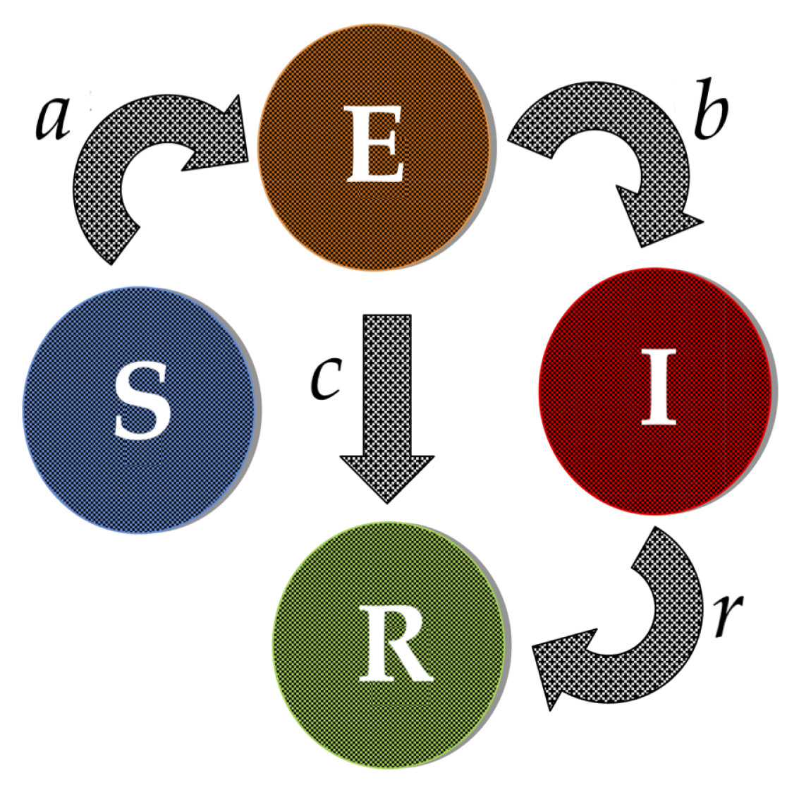
Figure 2.
Plot of real and imaginary values of the eigenvalues of .
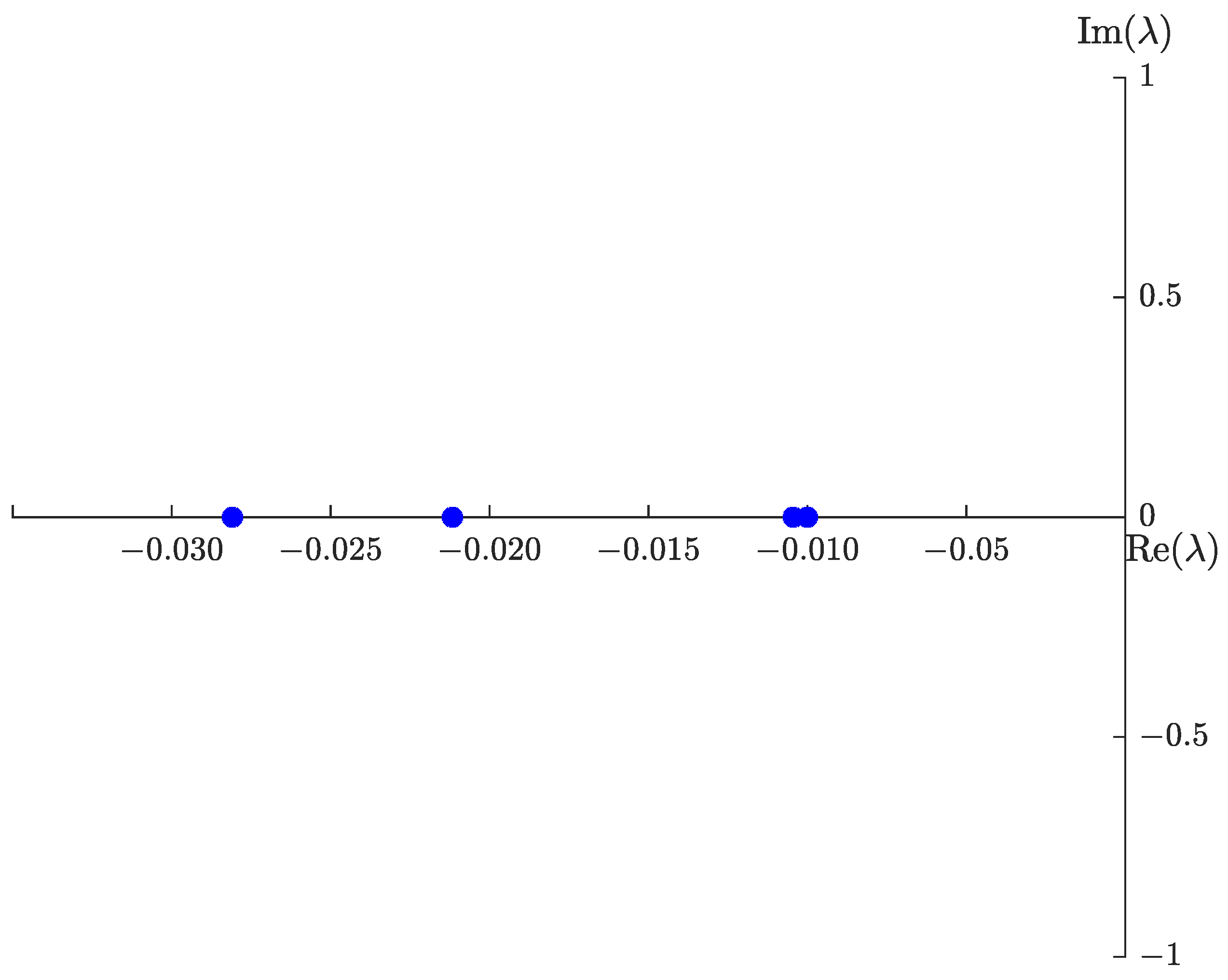
Figure 3.
Plot of real and imaginary values of the eigenvalues of , for .
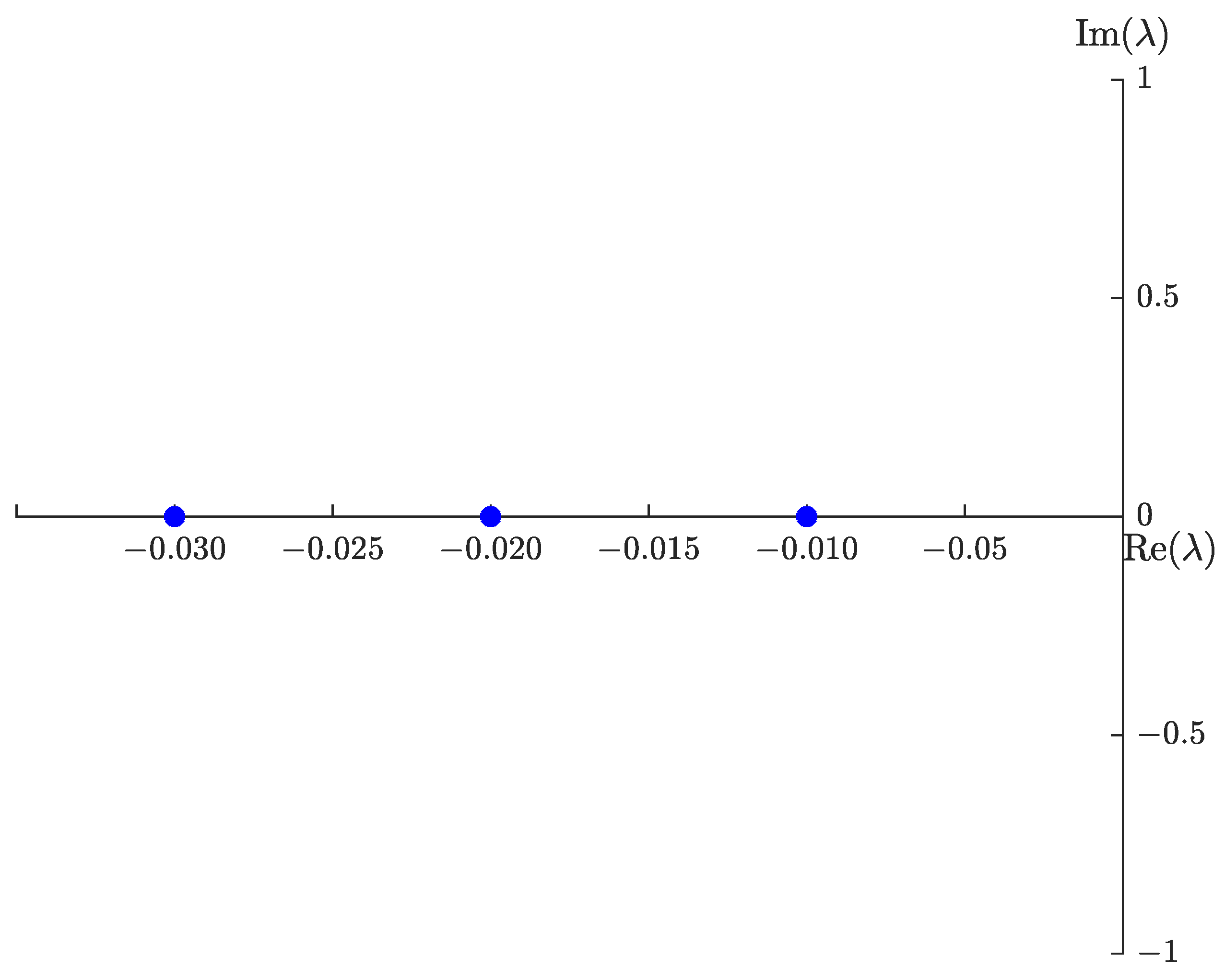
Figure 4.
Plot of real and imaginary values of the eigenvalues of , for .
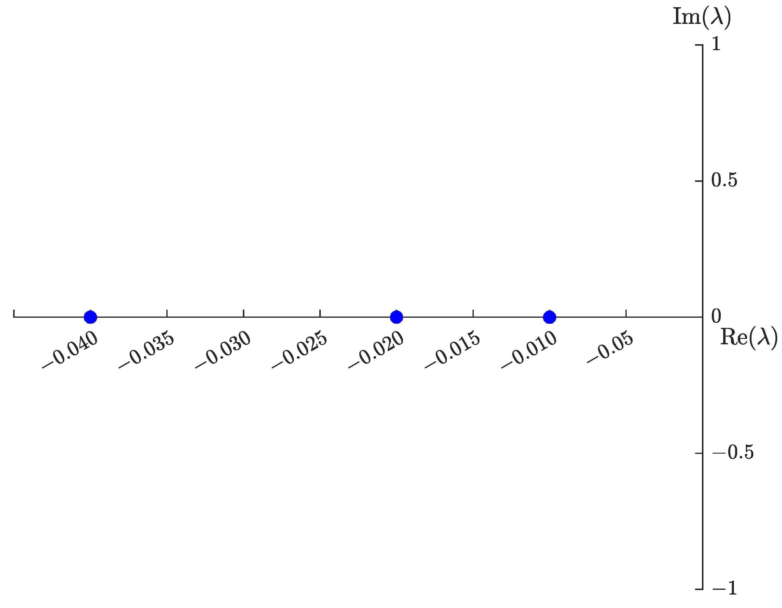
Figure 5.
Plot of real and imaginary values of the eigenvalues of , for .
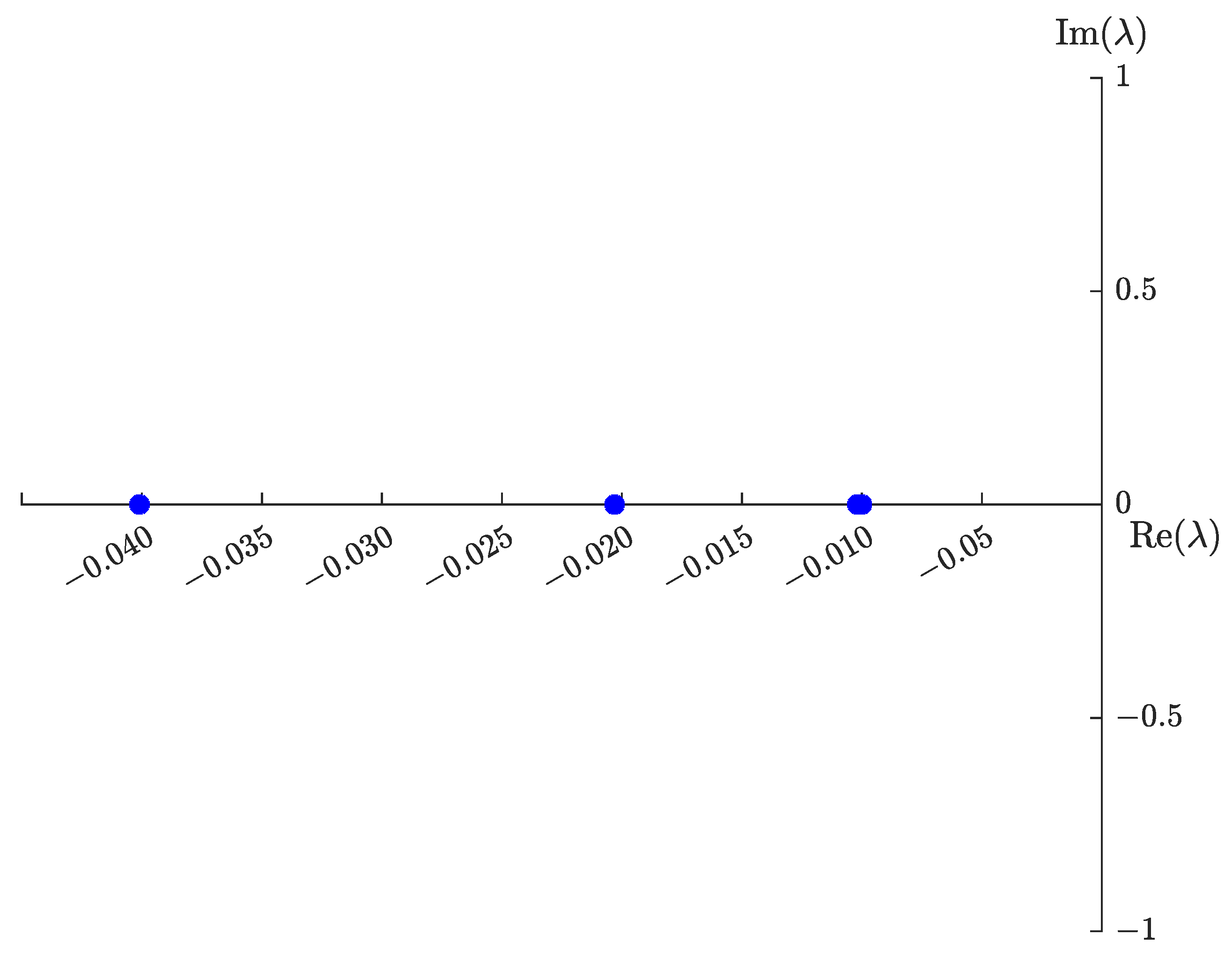
Figure 6.
Plot of the number of susceptible, exposed, infected, and recovered people over time t (in days) to show positivity of solutions on , , , and .
Figure 6.
Plot of the number of susceptible, exposed, infected, and recovered people over time t (in days) to show positivity of solutions on , , , and .

Figure 7.
Bar plot of values of the indicated sensitivity index and type of rate.
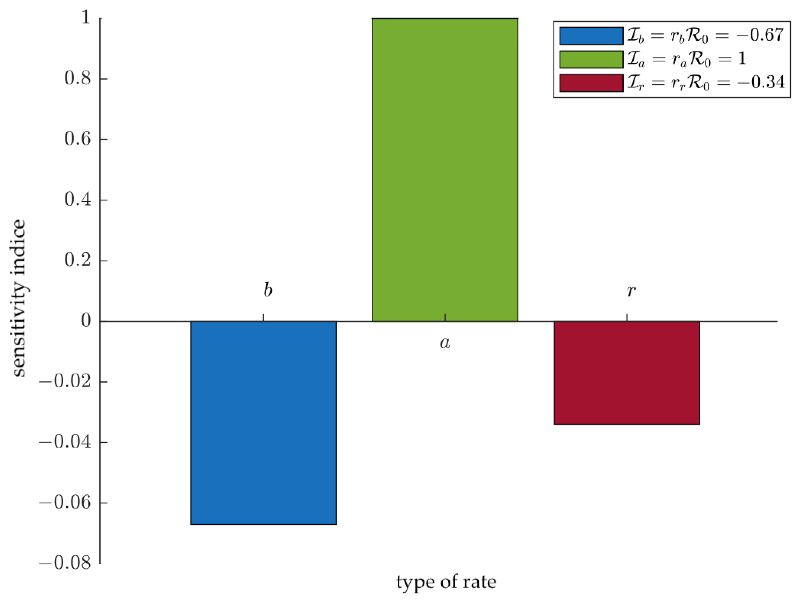
Figure 8.
Block diagram of the first-order vector initial value problem given in (1).
Figure 8.
Block diagram of the first-order vector initial value problem given in (1).
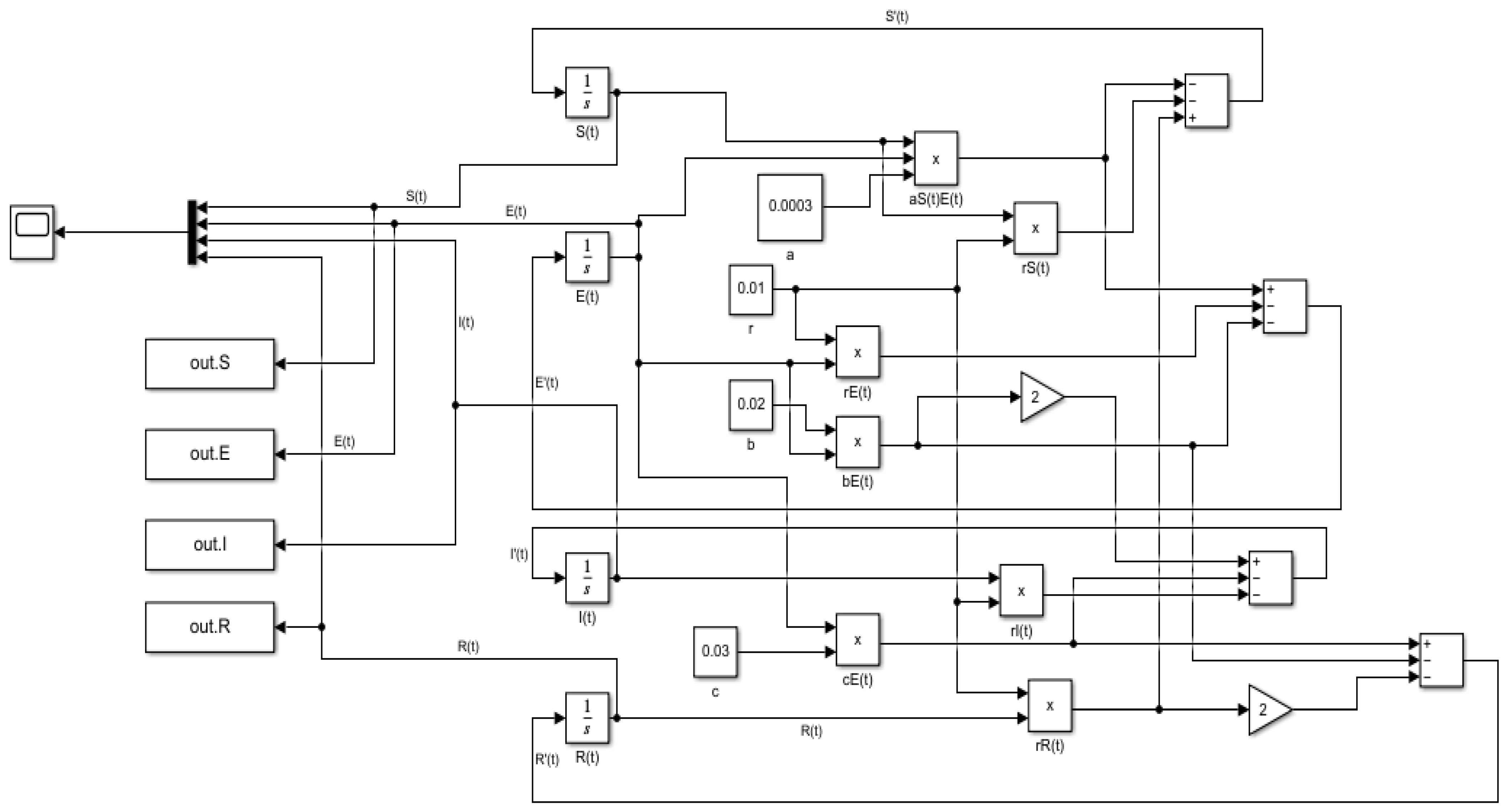
Figure 9.
Plot of the number of susceptible, exposed, infected, and recovered people, , , , and , over time t (in days) of the SEIR model for solutions based on first-order derivatives for all .
Figure 9.
Plot of the number of susceptible, exposed, infected, and recovered people, , , , and , over time t (in days) of the SEIR model for solutions based on first-order derivatives for all .
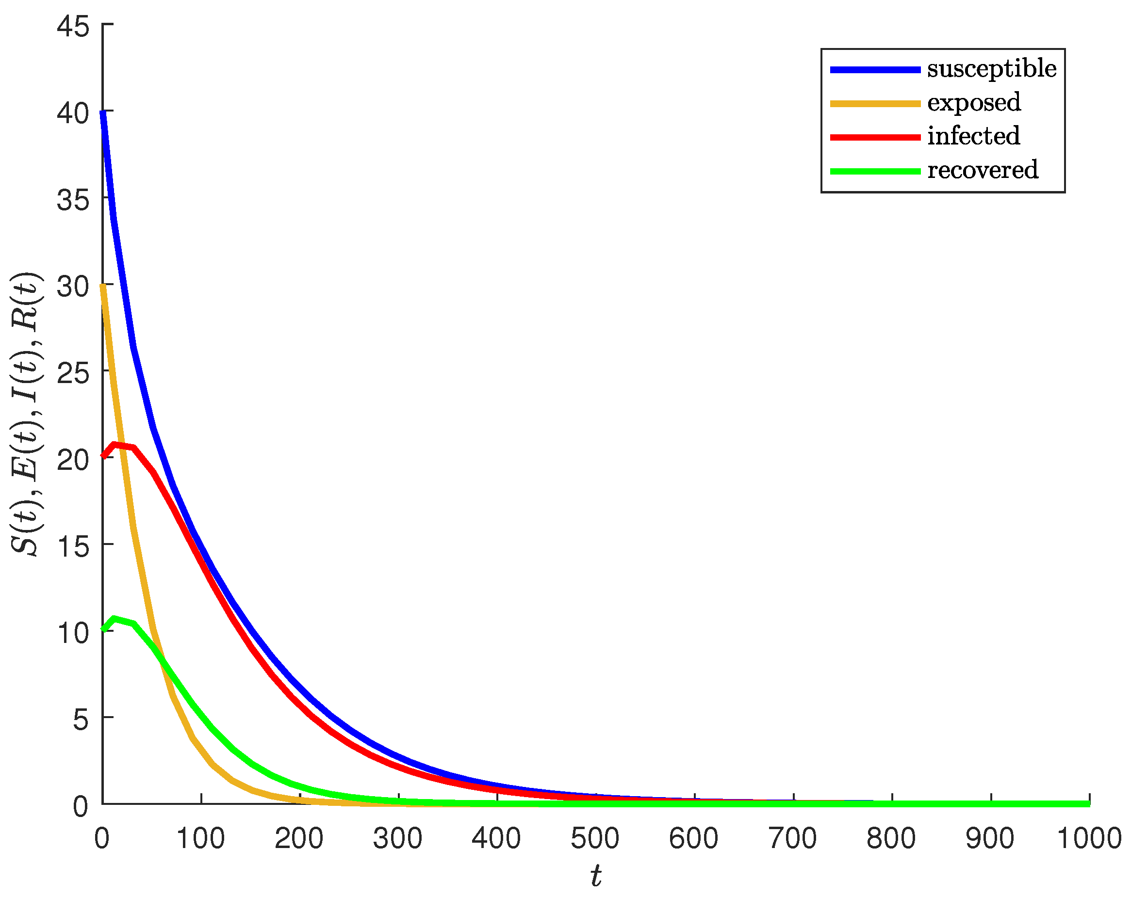
Figure 10.
Plots of the number of susceptible (a), exposed (b), infected (c), and recovered (d), cases over time (in days) for 11 solutions each based on the th fractional derivative with for all .
Figure 10.
Plots of the number of susceptible (a), exposed (b), infected (c), and recovered (d), cases over time (in days) for 11 solutions each based on the th fractional derivative with for all .


Table 1.
Notations/symbols employed in the SEIR model.
| Notations/Symbols | Definition |
|---|---|
| t | Time instant |
| Susceptible population at t | |
| Exposed population at t | |
| Infected population at t | |
| Recovered population at t | |
| Total population at t | |
| Initial susceptible population, (fixed) | |
| Initial exposed population, (fixed) | |
| Initial infected population, (fixed) | |
| Initial recovered population, (fixed) | |
| Initial total population | |
| Basic reproduction number | |
| a | Rate at which susceptible become exposed, (fixed) |
| b | Rate at which exposed become infected, (fixed) |
| c | Rate at which exposed become recovered, (fixed) |
| r | Rate at which infected become recovered, (fixed) |
Publisher’s Note: MDPI stays neutral with regard to jurisdictional claims in published maps and institutional affiliations. |
© 2022 by the authors. Licensee MDPI, Basel, Switzerland. This article is an open access article distributed under the terms and conditions of the Creative Commons Attribution (CC BY) license (https://creativecommons.org/licenses/by/4.0/).
Share and Cite
MDPI and ACS Style
Rangasamy, M.; Chesneau, C.; Martin-Barreiro, C.; Leiva, V. On a Novel Dynamics of SEIR Epidemic Models with a Potential Application to COVID-19. Symmetry 2022, 14, 1436. https://doi.org/10.3390/sym14071436
AMA Style
Rangasamy M, Chesneau C, Martin-Barreiro C, Leiva V. On a Novel Dynamics of SEIR Epidemic Models with a Potential Application to COVID-19. Symmetry. 2022; 14(7):1436. https://doi.org/10.3390/sym14071436
Chicago/Turabian StyleRangasamy, Maheswari, Christophe Chesneau, Carlos Martin-Barreiro, and Víctor Leiva. 2022. "On a Novel Dynamics of SEIR Epidemic Models with a Potential Application to COVID-19" Symmetry 14, no. 7: 1436. https://doi.org/10.3390/sym14071436
Note that from the first issue of 2016, this journal uses article numbers instead of page numbers. See further details here.