Hidden Homogeneous Extreme Multistability of a Fractional-Order Hyperchaotic Discrete-Time System: Chaos, Initial Offset Boosting, Amplitude Control, Control, and Synchronization

Abstract

Fractional order maps are a hot research topic; many new mathematical models are suitable for developing new applications in different areas of science and engineering. In this paper, a new class of a 2D fractional hyperchaotic map is introduced using the Caputo-like difference operator. The hyperchaotic map has no equilibrium and lines of equilibrium points, depending on the values of the system parameters. All of the chaotic attractors generated by the proposed fractional map are hidden. The system dynamics are analyzed via bifurcation diagrams, Lyapunov exponents, and phase portraits for different values of the fractional order. The results show that the fractional map has rich dynamical behavior, including hidden homogeneous multistability and offset boosting. The paper also illustrates a novel theorem, which assures that two hyperchaotic fractional discrete systems achieve synchronized dynamics using very simple linear control laws. Finally, the chaotic dynamics of the proposed system are stabilized at the origin via a suitable controller.

1. Introduction

While discrete fractional calculus was first introduced roughly fifty years ago, the non-integer-order derivative has been a mathematical idea since 1695 [1]. In particular, the discretization of continuous-time operators [2] in 1974 led to the first derivations of fractional differential equations. Due to the recent widespread interest in discrete fractional calculus, many difference operators, notably the Grünwald–Letnikov difference operator [3], have been proposed in the literature. Many efforts have been made to thoroughly analyze the dynamics of both classical systems and fractional systems since the discovery of chaos phenomena in dynamical systems [3,4]. Regarding the latter, various works have been conducted on the topic of studying chaotic behaviors in nonlinear maps defined by fractional order difference equations [5,6,7]. Wu et al. [8] proposed a fractional logistic map and studied the chaotic behavior based on the Caputo-left difference operator. One-dimensional fractional maps with chaotic attractors and quasi-periodic behaviors were suggested in [9]. Further evidence for chaotic attractors was provided by Khennaoui et al. [10] in three fractional maps, namely the Wang map, the Stefanski map, and the Rössler map. The dynamic behavior of a higher-dimensional fractional-order chaotic map was described by Peng et al. in [11] that same year, while Wang et al. examined the chaos and complexity of a fractional order higher-dimensional multi-cavity chaotic map in [12]. Memristive maps with integer and fractional orders have recently been proposed [13,14]. A memristor-based Rulkov neuron map was introduced in [15] by using a discrete memristor to replicate the magnetic effects, whereas [16] illustrated the dynamic features of a novel discrete memristive hyperchaotic map.

Compared with integer-order chaotic maps, fractional-order chaotic maps have more complex dynamic characteristics, i.e., where a parameter can increase the degree of freedom of the model. These additional degrees of freedom can also be employed to uncover the subtleties of ecological processes that occur in the real world. In order to better understand these complex dynamical characteristics, more discrete maps with fractional operators must be provided. Furthermore, one of the distinctive benefits of fractional-order maps is that they are sensitive to variations in fractional orders in addition to tiny perturbations in parameters and initial circumstances. Additionally, fractional-order discrete maps are advantageous for system analysis and numerical computation because they have straightforward forms and rich dynamics.

In recent years, coexisting attractors and hidden attractors have been reported in various chaotic fractional maps. For example, in [17], the presence of chaos in fractional discrete systems with rectangle-shaped and square-shaped fixed points was investigated; ref. [18] provided an illustration of the behavior of a discrete fractional-order Bonhoeffer-van der Pol oscillator. The coexistence of various attractors, such as chaotic and hyperchaotic attractors as well as quasi-periodic and periodic attractors, is highlighted by the map. Furthermore, Almatroud et al. [19] showed that a brand-new 2D fractional-order chaotic map included hidden extreme multistability. A fractional discrete system without fixed points is provided in [20]. To demonstrate the existence of chaotic hidden attractors in the system dynamics, the 0–1 test and the computation of the approximation entropy have been used. Later, using bifurcation diagrams, Lyapunov exponents, and a 0–1 test, the complex dynamic behaviors of a fractional map with hidden attractors were addressed; see [21]. The synchronization and control of the system dynamics are also suggested. A synchronized chaotic system aims to achieve the state of a chaotic master system. Hence, $t\to +\infty$ gives us a synchronization error that converges toward zero. The design of synchronization schemes is influenced by a wide range of techniques. The chaos synchronization phenomenon was studied in many different ways, such as hybrid projection synchronization, inverse matrix projection synchronization, Q–S synchronization, complete synchronization, etc. [22,23,24].

In this study, a discrete-time new fractional system with the line of equilibrium and no equilibrium points was constructed with the following properties: homogeneous multistability, hidden dynamics, and amplitude control. This new fractional-order hyperchaotic map possesses not only hidden attractors but also coexisting attractors. The initial boosting phenomena were investigated in the proposed hyperchaotic map, as seen in Section 3, with an independent knob for partial amplitude control in Section 4. A suitable controller stabilizes the hyperchaotic system in Section 5. A novel theorem is presented in Section 6, which claims that two fractional hyperchaotic systems can be controlled linearly to show synchronized dynamics. Our conclusions with ideas for future work are presented in Section 7.

2. Description and Analysis of the Fractional Hyperchaotic Map

Recently, Bao et al. [25] proposed a new hyperchaotic map by introducing the nonlinear sinus function into a simple map, which is governed by Equation (1). As shown below, it has only one nonlinear term and two real constants controllers A and B:

$$\left\{\begin{array}{c}{x}_1(n+1)=x_1\left(n\right)+A{x}_1\left(n\right)sin{x}_2\left(n\right)+B,\hfill \\ x_2(n+1)=x_1\left(n\right)+x_2\left(n\right).\hfill \end{array}\right.$$

(1)

Inspired by some relevant works on fractional-order discrete-time system(s) (FODTS) [26], we define the fractional-order case by introducing the $\eta$-Caputo difference operator given by:

$$\begin{array}{c}{}^C{\Delta }_a^{\eta }g\left(s\right)=\frac{1}{\eta \left(m-\eta \right)}\sum _{\tau =a}^{s-\left(m-\eta \right)}{\left(s-\tau -1\right)}^{\left(m-\eta -1\right)}{\Delta }_{\tau }^{m}g\left(\tau \right),\hfill \end{array}$$

(2)

where $s\in {\mathbb{N}}_{a+m-\eta }$, $m=⌈\eta ⌉+1$ and $\eta \notin \mathbb{N}$. The corresponding fractional-order form is built as follows

$$\left\{\begin{array}{c}{}^C{\Delta }_a^{\eta }{x}_1\left(s\right)=A{x}_1(s-1+\eta )sin{x}_2(s-1+\eta )+B,\hfill \\ {}^C{\Delta }_a^{\eta }{x}_2\left(s\right)=x_1(s-1+\eta ),\hfill \end{array}\right.$$

(3)

where $s\in {\mathbb{N}}_{a+1-\eta }$ and $\eta \in (0,1]$ are the fractional orders. The 2D FODTS (3) is symmetric with respect to the plane $S=\{(x_1,x_2)\in \mathbb{R},x_1=0,x_2=0\}$, and control parameters A and B, where it is always invariant under the transformation $\left(x_1,x_2,A,B\right)\to \left(-x_1,-x_2,-A,-B\right)$. Thus, the attractor of the proposed FODTS could display symmetric behavior.

The equilibrium points of the FODTS (3) are easily determined from:

$$\left\{\begin{array}{c}A{x}_{1}sin{x}_2+B=0,\hfill \\ x_1=0.\hfill \end{array}\right.$$

(4)

Similar to the integer-order counterpart, two different cases are considered:

Case a: when $B\ne 0$ Equation (4) has no solution, demonstrating that the fractional map (3) has no equilibrium point.

Case b: when $B=0$, the fixed points of the FODTS (3) are given by $L=\left(0,C\right);$ where C is a real number. In other words, the proposed system has line equilibrium points. The Jacobian matrix $\left(Jac\right)$ for system (3), computed at L, is:

$$Jac=\left[\begin{array}{cc}AsinC& 0\\ 1& 0\end{array}\right],$$

(5)

whose determinant is equal to zero $(detJac=0)$. According to the stability theorem of a fractional-order discrete-time system [19], the line of the equilibrium point is stable if

$$\left\{\begin{array}{c}\frac{-Tr\left(Jac\right)}{2}\ge \sqrt{Det\left(Jac\right)},\hfill \\ \eta >lo{g}_2\frac{\sqrt{Tr{\left(Jac\right)}^2-4Det\left(Jac\right)}-Tr\left(Jac\right)}{2},\hfill \\ Det\left(Jac\right)>0\hfill \end{array}\right.$$

(6)

The conditions $\frac{-Tr\left(Jac\right)}{2}\ge \sqrt{Det\left(Jac\right)}$ and $Det\left(Jac\right)>0$ cannot be satisfied at the same time; thus, system (3) has a high possibility of hidden attractors.

By definition, all chaotic attractors generated by the proposed FODTS (4) are hidden attractors.

3. Dynamical Analysis and Numerical Simulations

Nonlinear dynamical analysis tools, such as phase diagrams, bifurcation diagrams, and Lyapunov exponents are used to analyze the hidden dynamics. We shall first give the numerical formula of the proposed map. By applying the $\eta$ fractional sum, ${\Delta }_{\tau }^{-\eta }g\left(\tau \right)=\frac{1}{\mathsf{\Gamma }\left(\eta \right)}{\sum }_{\tau =a}^{s-\gamma }{\left(s-\tau -1\right)}^{\left(\gamma -1\right)}g\left(\tau \right)$, the numerical formula is designed as:

$$\left\{\begin{array}{c}{x_1}_n={x_1}_0+\frac{1}{\mathsf{\Gamma }\left(\eta \right)}\sum _{j=0}^{n-1}\frac{\mathsf{\Gamma }(n-1-j+\eta )}{\mathsf{\Gamma }(n-j)}A{x_1}_{j}sin{x_2}_j+B,\hfill \\ {x_2}_n={x_2}_0+\frac{1}{\mathsf{\Gamma }\left(\eta \right)}\sum _{j=0}^{n-1}\frac{\mathsf{\Gamma }(n-1-j+\eta )}{\mathsf{\Gamma }(n-j)}{x_1}_j.\hfill \end{array}\right.$$

(7)

As one can see from Equation (7), the proposed FODTS (3) has the memory effect. Hence, the states ${x_1}_n,{x_2}_n$ depend on $x_0,x_1,x_2,\dots ,x_{n-1}$.

Using numerical simulations of the same bifurcation parameters for the integer-order map reported in [25], we present the dynamics of the suggested fractional-order map in order to find hidden chaotic attractors.

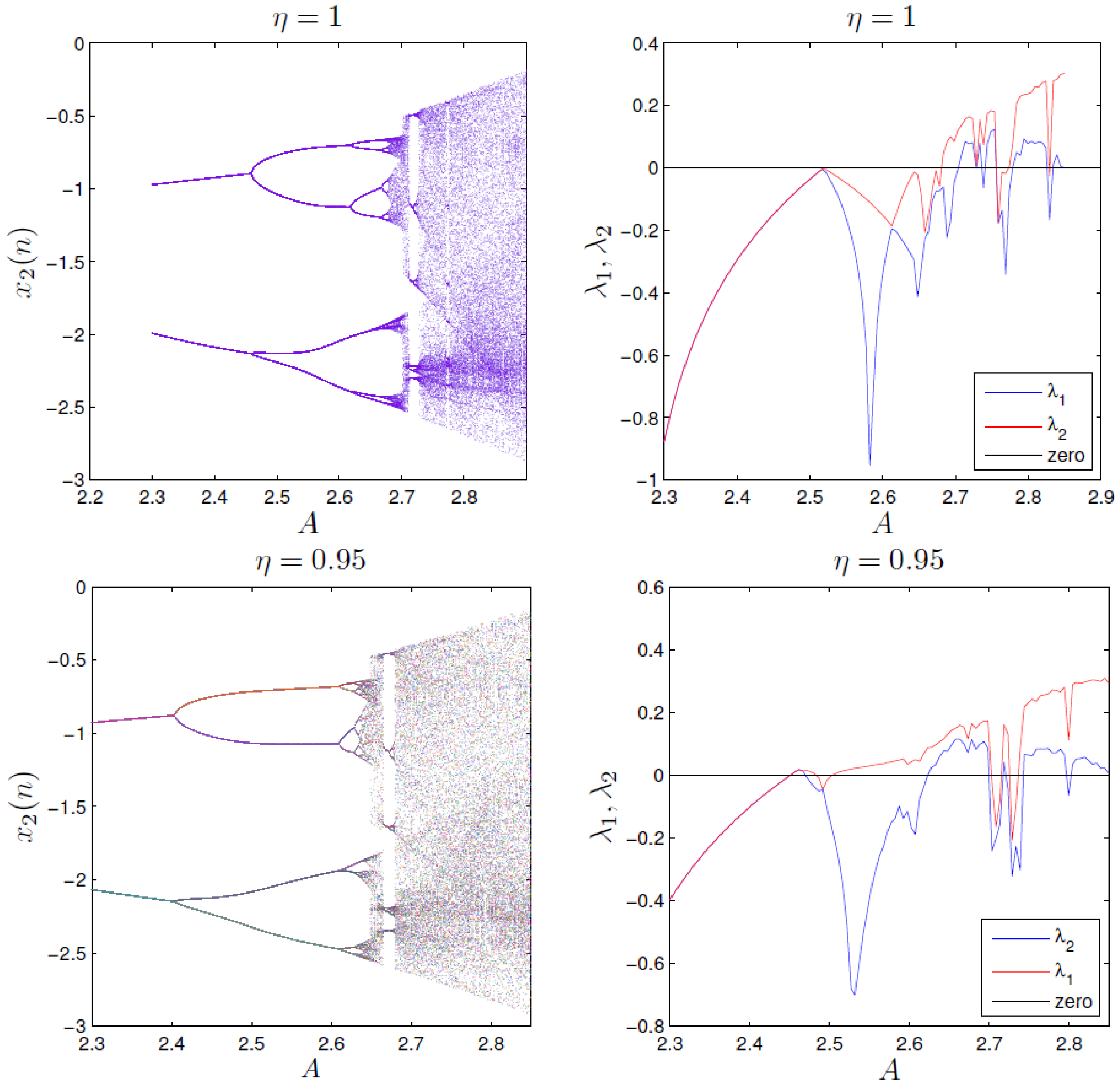
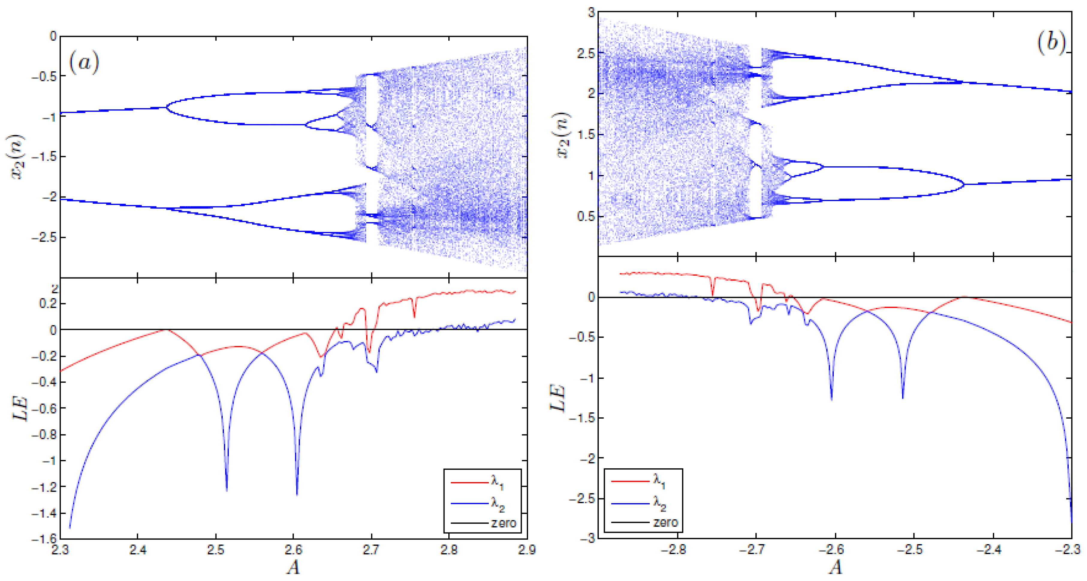
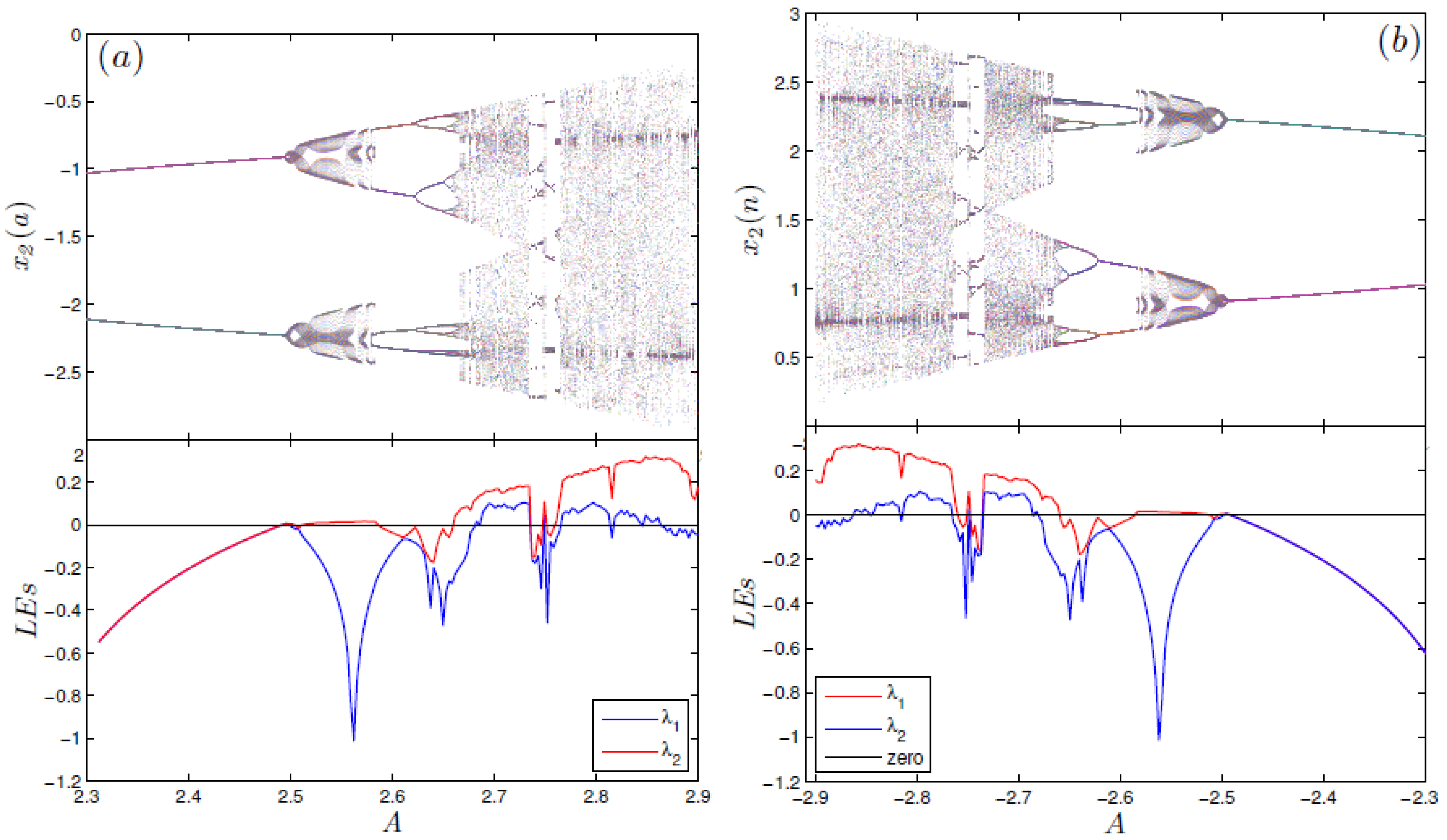
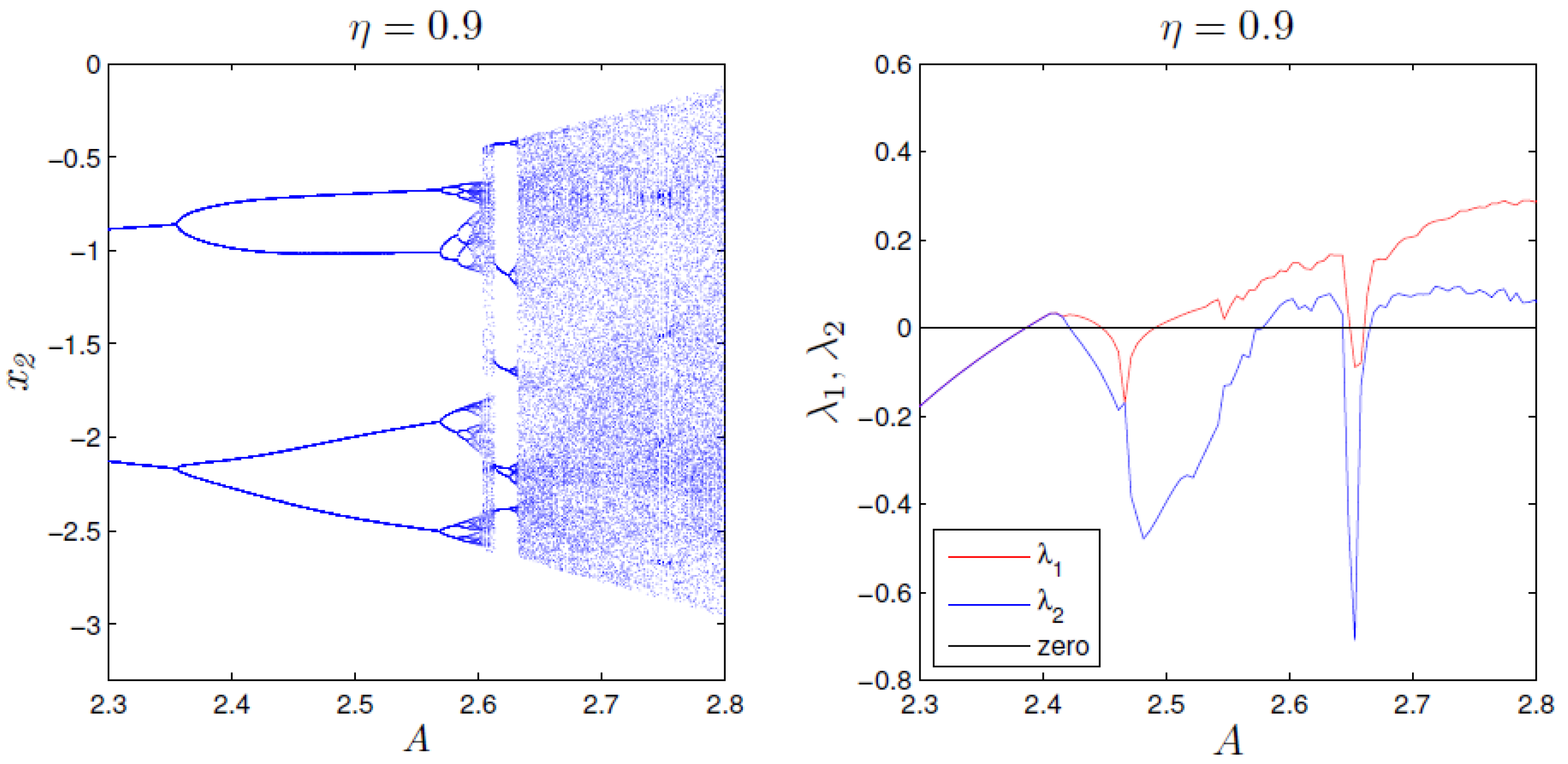
3.1. Hidden Attractors and Bifurcation Analysis

The control parameter B is assigned as $B=\pm 0.1$, $B=0$, respectively, and the initial condition is selected as ${x_1}_0=\pm 1,{x_2}_0=\pm 2$, respectively. The properties of the coexisting symmetrical hidden attractors are illustrated by considering the bifurcation diagrams and Lyapunov exponents (LEs) for $A\in [2.3,2.9]$ and $A\in [-2.9,-2.3]$, respectively. The bifurcation diagram is obtained by plotting the local maxima of the state $x_2$ in terms of the control parameter A, whereas the LEs are computed numerically using the Jacobian matrix algorithm. The LEs are computed numerically using the Jacobian matrix algorithm for fractional maps [27].

• Case A: No Fixed Point

$B=0.1$ and the initial values ${x_1}_0=1$, ${x_2}_0=-2$; the bifurcation diagram and the corresponding LEs are plotted in Figure 1a. These diagrams are obtained for $\eta =0.98$ and for $A\in [2.3,2.9]$. From the LEs and bifurcation diagram in Figure 1a, it can be seen that the FODTS (3) gradually changes from the periodic state to a chaotic state at $A\in [2.665,2.692]\cup [2.704,2.85]$, to a hyperchaotic state for $A\in [0.8,0.9286]$, through period-doubling. With the change of system parameter A, the LE diagram approves the dynamic behavior observed in the bifurcation diagram.

Figure 1. Bifurcation diagrams and LEs of the FODTS (3) with no equilibria for fractional order value $\eta =0.98$: (a) for $A\in [2.3,2.9]$; $B=0.1$, and initial value ${x_1}_0=1;{x_2}_0=-2$; (b) for $A\in [-2.9,-2.3]$; $B=-0.1$, and initial value ${x_1}_0=-1;{x_2}_0=2$.

In contrast, when the control parameter B is fixed as $B=-0.1$ and the initial values are set to ${x_1}_0=-1$, ${x_2}_0=2$, while the control parameter A changes in the range $[-2.9,-2.3]$; the FODTS (3) also shows the period-doubling route to chaos. Namely, the FODTS (3) is chaotic when $A\in [2.665,2.692]\cup [2.704,2.85]$, where $max\lambda$ is positive, and is in hyperchaos when $A\in [0.8,0.9286]$; where ${\lambda }_1,{\lambda }_2>0$. Basically, Figure 1 shows that under symmetrical initial values, the dynamic evolution of the FODTS caused by the symmetrical control parameters $A\in [2.3,2.9]$ and $A\in [-2.9,-2.3]$, respectively, had symmetrical similarity.

To observe the coexistence of hidden symmetric attractors in the FODTS (3), the phase portraits, as seen in Figure 1, are disposed of in Figure 2. Red trajectories were obtained for the constant parameter $B=0.1$, fractional order $\eta =0.98$, and the initial values ${x_1}_0=1,{x_2}_0=-2$; blue trajectories were obtained for $B=-0.1$, $\eta =0.98$, ${x_1}_0=-1,{x_2}_0=2$. For different values of A, the FODTS shows symmetrical hidden periodic attractors, symmetrical hidden chaotic attractors, and symmetrical hidden hyperchaotic attractors. Therefore, it is concluded that the FODTS has complex hidden dynamics. Moreover, the coexistence behavior indicates the sensitivity of the map (3) to the control parameters and initial values.

Figure 2. Hidden attractors of the FODTS (3) for the symmetrical initial conditions $\left({x_1}_0,{x_2}_0\right)=(\pm 1,\pm 2)$, fractional order $\eta =0.98$, positive system parameters in red diagrams, and negative system parameters in blue diagrams: (a) hidden periodic attractors for $A=\pm 2.62$ and $B=\pm 0.1$; (b) hidden chaotic attractors for $A=\pm 2.772$ and $B=\pm 0.1$; (c) hidden hyperchaotic attractors for $A=\pm 2.85$ and $B=\pm 0.1$.

• Case B: Line of the Equilibrium Point

As the system parameters and the initial state variables of the 2D fractional system are taken as $B=0$, ${x_1}_0=1,{x_2}_0=-2$, the bifurcation diagrams along with the LEs diagram for the fractional order value $\eta =0.95$ are shown in Figure 3a. As illustrated in the previous section, when $B=0$, the FODTS (3) has a line of equilibria. When the bifurcation A increases from 2.3 to 2.9, it can be seen from the bifurcation diagram that the FODTS starts from the period and goes into chaos via the cascade of period-doubling bifurcation and then turns into hyperchaos at interval $A\in [2.689,2.734]\cup [2.77,2.813]$. In contrast, when the parameter A is adjusted in the region $[-2.9,-2.3]$, the bifurcation of the state $x_2$ and the LEs are numerically simulated as shown in Figure 3b. Similarly, it is easily viewed that the bifurcation diagram in Figure 3b had certain symmetrical similarities with the one reported in Figure 3a. Therefore, it proves that the coexistence behavior appears in the hidden attractors of the FODTS with the lines of the equilibrium points.

Figure 3. Bifurcation diagrams and Lyapunov exponents of the FODTS (3) with the lines of the equilibrium points in the $A-x_2$ plane for the fractional order value $\eta =0.98$: (a) for $A\in [2.3,2.9]$; $B=0$, and IV $x_{10}=1;x_{20}=-2$; (b) for $A\in [-2.9,-2.3]$; $B=0$, and initial conditions $x_{10}=-1;x_{20}=2$.

Without loss of generality, the hidden attractors at several critical values corresponding to Figure 3 are shown in Figure 4.

Figure 4. Hidden attractors of the FODTS (3) with the lines of the equilibrium points for the symmetrical IV $(x_{10},x_{20})=(\pm 1,\pm 2)$, fractional order $\eta =0.98$, and positive system parameters in red, and negative system parameters in blue with $B=0$: (a) hidden periodic attractors for $A=\pm 2.752$, (b) hidden hyperchaotic attractors for $A=\pm 2.797$, (c) hidden chaotic attractors for $A=\pm 2.867$.

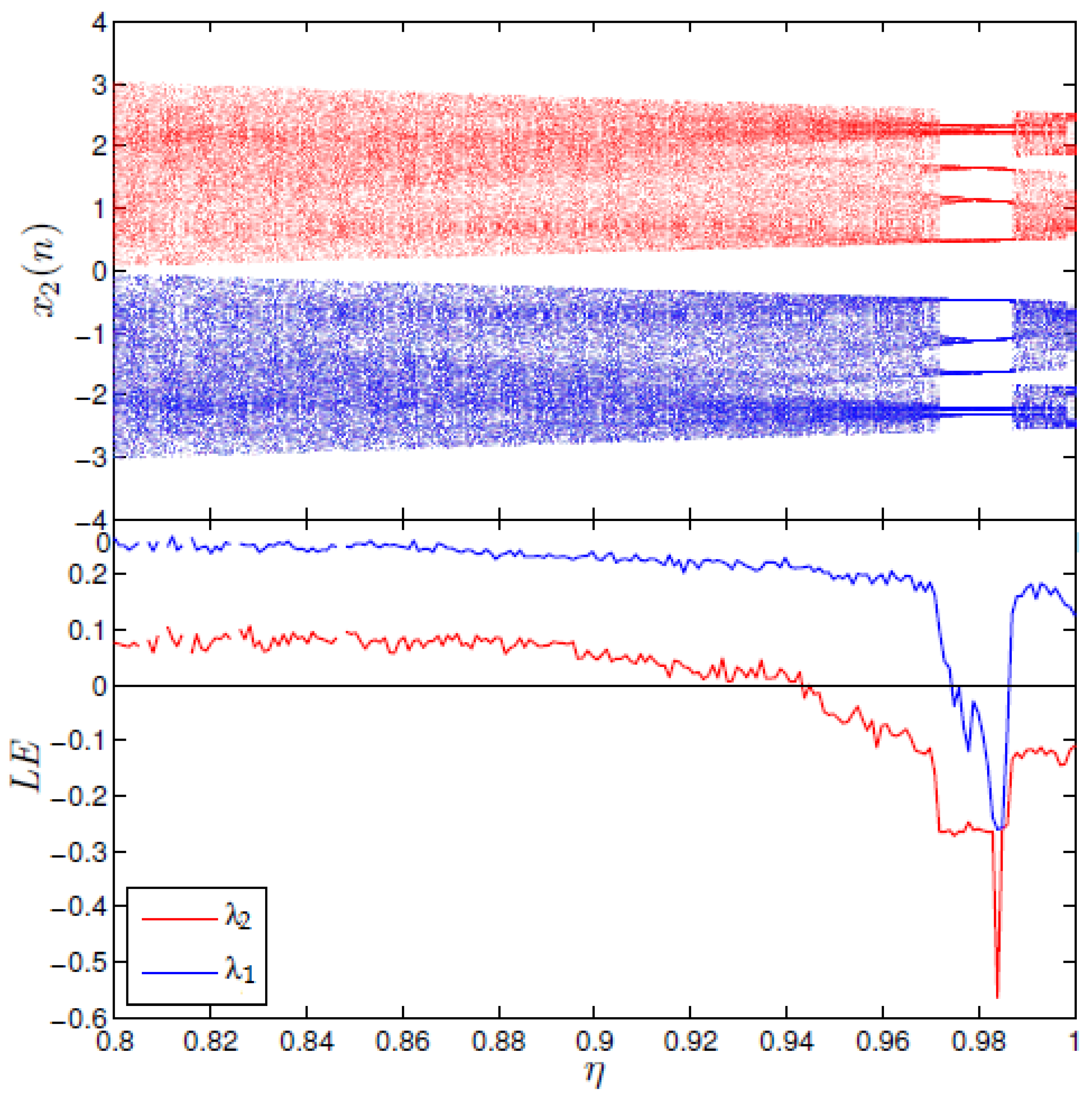
3.2. The Effect of Fractional Order $\eta$

In order to further understand the dynamics of the FODTS, the fractional order $\eta$ is considered a bifurcation parameter, and the bifurcation diagram along with the LEs are derived as shown in Figure 5. Note that the blue diagram is obtained for the initial condition $(1,-2)$ and system parameters $A=2.7,B=0.1$, while the red diagram is obtained for $A=-2.7$, $B=-0.1$, with initial conditions ${x_1}_0=-1$, ${x_2}_0=2$. It is observed that the new FODTS produces more complex dynamics compared with the integer-order map (1). In particular, for the corresponding integer-order value $\eta =1$, the FODTS is chaotic where the maximum LEs is bigger than 0. However, it becomes hyperchaotic as the fractional order value decreases, where both of the Lyapunov exponents $(L{E}_1,L{E}_2)$ become bigger than 0, which indicates that the dynamic characteristic of the FODTS is more complex. Moreover, when $\eta \in [0.8,0.9286]$, the FODTS (3) is in hyperchaos, where ${\lambda }_1,{\lambda }_2>0$ with some unbounded region for the largest values of n. When $\eta \in [0.9286,0.9739]\cup [0.9869,1]$ the FODTS is in chaos, where $max\lambda >0$. The phase portraits for the fractional order values $\eta =0.9$ and $\eta =1$, which are associated with the hidden hyperchaotic and hidden chaotic attractors, respectively, are illustrated at the top of Figure 5.

Figure 5. Hidden attractors, bifurcation diagrams, and Lyapunov exponents (LEs) versus $\eta$ of the FODTS (3) for the symmetrical initial conditions $({x_1}_0,{x_2}_0)=(\pm 1,\pm 2)$, and positive control parameter $A=2.7$, $B=0.1$ (red diagram), and negative control parameters $A=-2.7$, $B=-0.1$ (blue diagram).

The bifurcation diagram and LEs are used to analyze the relationship between the control parameter A and the fractional order $\eta$. When the system parameter A is adjusted in the region $[2.2,2.9]$, the fractional order $\eta$, respectively, is selected as $\eta =0.9$, $\eta =0.95$, $\eta =1$. Three kinds of bifurcation diagrams are depicted in Figure 6, with different color regions. Correspondingly, the LEs are calculated and shown in Figure 6. The dynamic behavior of the FODTS depends on the value of the control parameter A and the value of $\eta$. Figure 6 shows that the states of the FODTS (3) go from a periodic to a chaotic state with the decrease of order $\eta$, as A increases and $\eta$ decreases, it is observed that the chaotic band suddenly disappears and the system goes into infinity. The LE diagrams confirm that the system passes from periodic regions to chaotic and hyperchaotic regions as the system parameter A increases, and the fractional order value decreases.

Figure 6. Different bifurcation diagrams and Lyapunov exponents of the FODTS (3) with the variation of control parameter A and fractional order $\eta$.

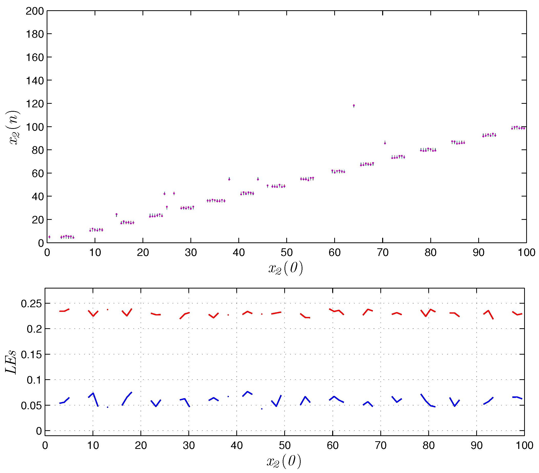
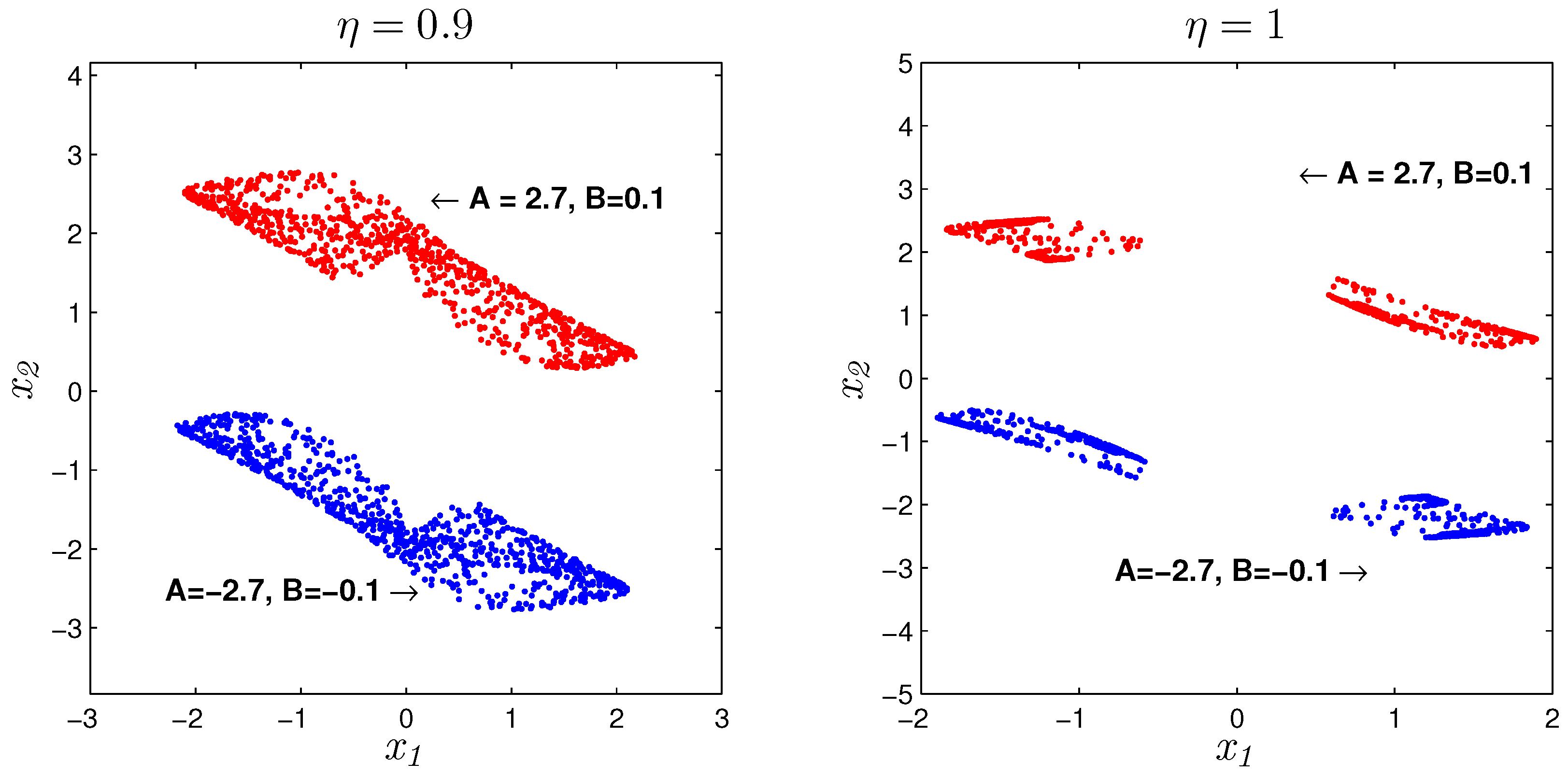
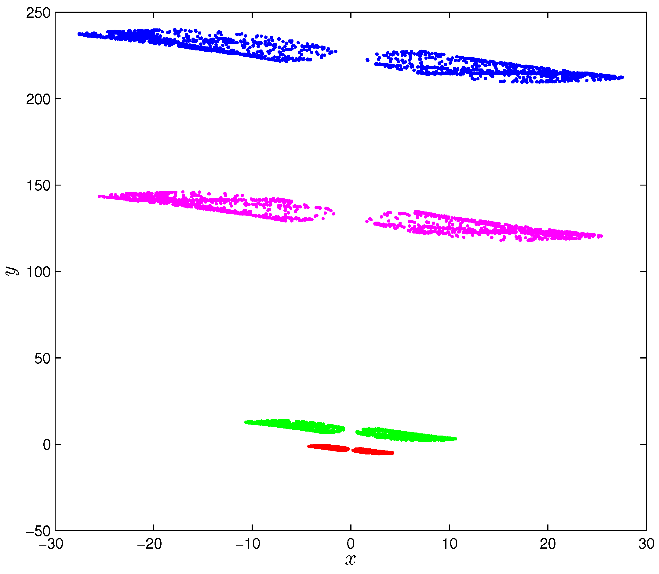
3.3. Hidden Extreme Homogeneous Multistability

To reveal the extreme multistability of the FODTS (3), the maximum LEs and the bifurcation diagrams of the state variable ${x_2}_n$ are calculated as shown in Figure 7, where the fractional order $\eta$ is chosen as $0.98$. The parameters are selected as $A=2.7$, $B=0.1$, and the IV is fixed as ${x_1}_0=1$, while ${x_2}_0$ varies in the range $[0,200]$. As shown in Figure 7, when $\eta =0.98$, system (3) generates multiple chaotic attractors along the $x_2$ axis, where the values of the LEs of the FODTS (3) are nearly the same, which indicates that all of these attractors have very close chaotic features. To exhibit the phenomenon of multistability, typical hyperchaotic attractors of the FODTS (3) with no equilibrium for a different IV ${x_2}_0$ are simulated, as shown in Figure 8. As can be seen, different initial condition values ${x_2}_0$ lead to different hidden hyperchaotic attractors of the same shape. This special phenomenon is known as homogeneous multistability, which is a new phenomenon in nonlinear systems [28]. The hidden homogeneous multistability of the FODTS (3) (with respect to small changes of the initial state ${x_2}_0$) is illustrated. Note that there are many other hidden hyperchaotic attractors with unified LEs for other IVs.

Figure 7. Bifurcation and LEs of the FODTS (3) versus IV ${x_2}_0$, for parameter values $A=2.7$, $B=0$ and fractional order $\eta =0.98$.

Figure 8. Five coexisting hidden hyperchaotic attractors for different initial conditions and control parameters $A=2.7,B=0.1$ and order $\eta =0.98$, $x_{20}=1$.

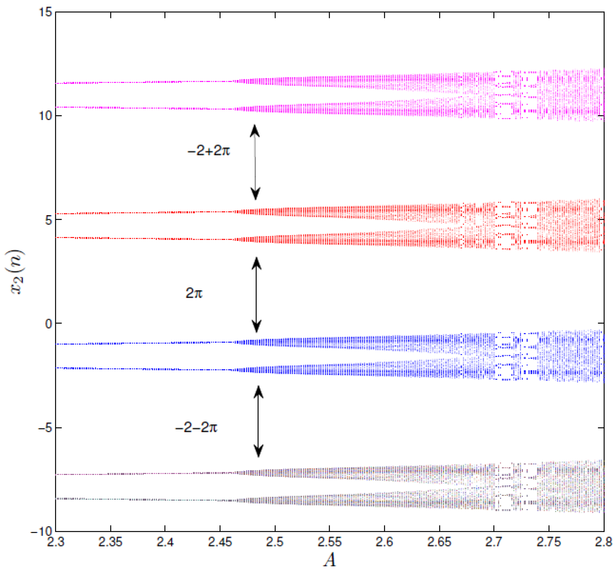
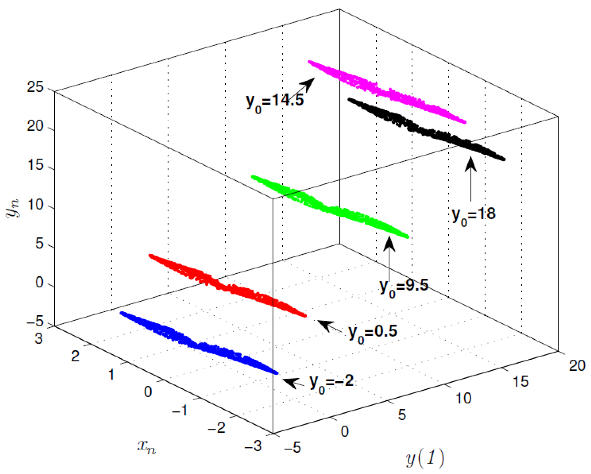
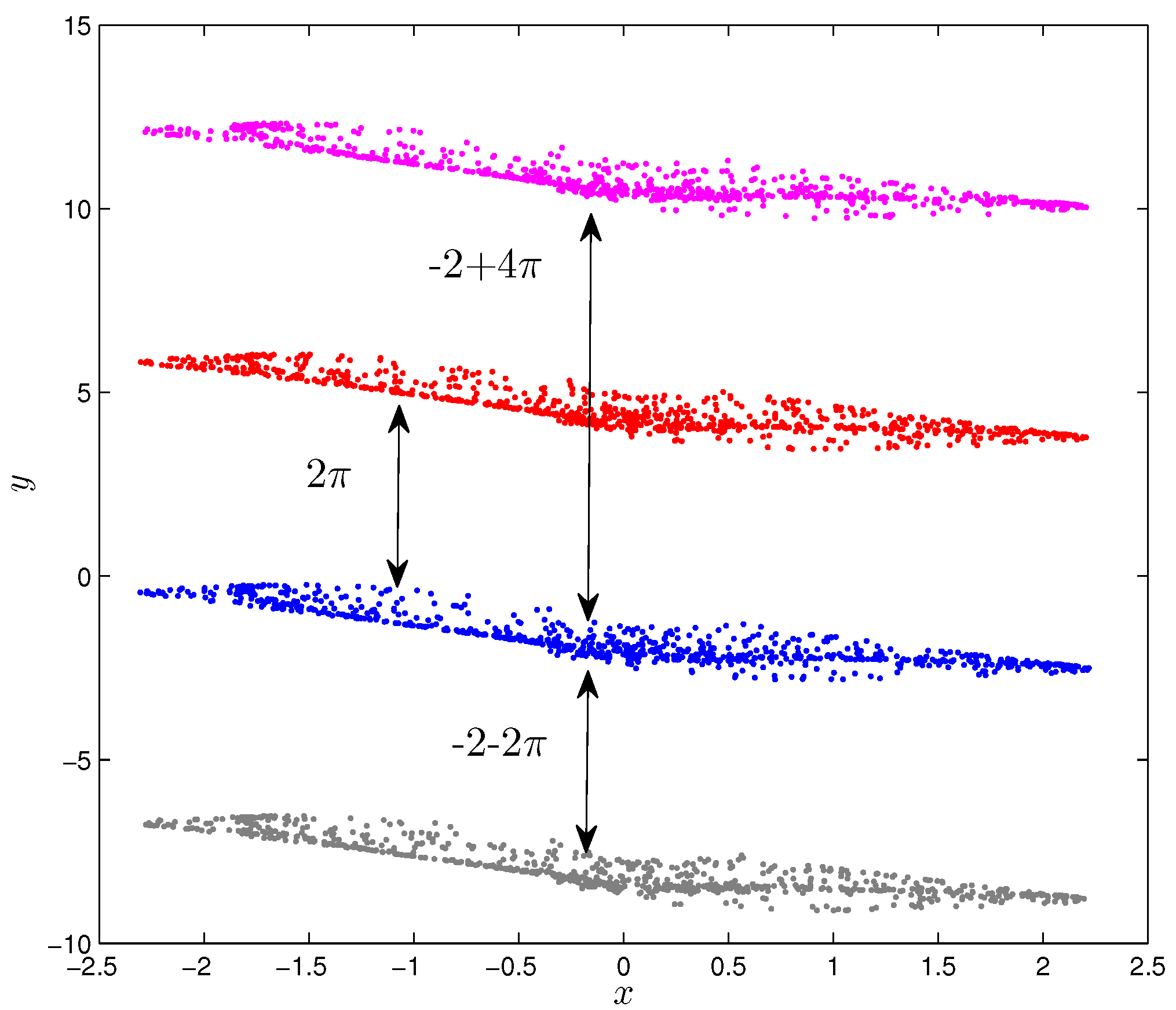
3.4. Initial Offset Boosting

In the following, we will discuss an unusual phenomenon of the new FODTS, namely the initial offset boosting by changing the IV ${x_2}_0$ with the $2\pi$ period as $x_{2}0=-2+2K\pi$ with the fixed order $\eta =0.95$, where $K=-1,0,1,2$ and ${x_1}_0=1$. In Figure 9, we present the bifurcation diagrams of system (3) when $A\in [2.3,2.9]$ and $B=0$. For four different values of IC ${x_2}_0$, the FODT systems experience four bifurcation diagrams with periods $2\pi$. All of these diagrams have the same structure with the $2\pi$ regime of homogenous multistability. The same result can be obtained if we consider the second case $B\ne 0.1$.

Figure 9. Offset boosting of the fractional map (3) for varying initial condition $y\left(0\right)$ with $x\left(0\right)=1$ and fractional order $\mu =0.95$. Bifurcation diagrams as the control parameter a increases in $[2.3,2.9]$ and $b=0.1$.

Fix $A=2.8$, $B=0.1$, and let the fractional order $\eta =0.95$; the hidden chaotic attractors are illustrated in Figure 10 for ${x_2}_0=-2+2K$. These hidden chaotic attractors have the same shape as regime $2\pi$.

Figure 10. Four hidden chaotic attractors with ${x_2}_0=-2-2\pi$ (grey), ${x_2}_0=-2$ (blue), ${x_2}_0=-2+2\pi$ (red), ${x_2}_0=-2+4\pi$ (magenta).

4. Amplitude Control Analysis

In this section, the amplitude control method is used to detect coexisting attractors of the FODTS (3). Amplitude control has potential application value in engineering applications because it can achieve stability and explain the unpredictable behaviors that occur in engineered systems [29,30,31].

It is very interesting that the proposed FODTS possesses the property of amplitude control, which means that the amplitudes of one or both states of the map are adjusted. By introducing a controlled parameter $c_1$ into the variable $x_2$, respectively, the FODTS (3) can be changed to

$$\left\{\begin{array}{c}{}^C{\Delta }_a^{\eta }{x}_1\left(s\right)=A{x}_1(s-1+\eta )sin\left(x_2(s-1+\eta )\right)+B,\hfill \\ {}^C{\Delta }_a^{\eta }{x}_2\left(s\right)=\frac{x_1(s-1+\eta )}{c_1},\hfill \end{array}\right.$$

(8)

which is identical to Equation (3) with transformation $x_1=u$ and $x_2=c_{1}v$. Therefore, parameter $c_1$ proportionally controls the amplitude of the FODTS states $x_1$ and $x_2$ according to $c_1$. In order to discuss the new fractional discrete-time system (8) in terms of controller $c_1$, we fix $A=2.8$, $B=0.1$, $\eta =0.98$, and ${x_1}_0=1;{x_2}_0=-2$; while parameter $c_1$ takes the values $\{-5,2,12,13\}$. The phase diagrams are depicted in Figure 11. These diagrams have the same shape structure as regime $c_1$. In particular, from Figure 11, it can be seen that the chaotic attractor of system (8) is larger as $c_1$ increases. Nevertheless, there are other cases of coexisting attractors that depend on the control parameter $c_1$.

Figure 11. Rescaled phase diagrams under different total amplitude controllers $c_1$ of FODTS with ${x_1}_0=1,{x_2}_0=-2$, and fractional order $\eta =0.98$: $c_1=-5$ (green diagram), $c_1=2$ (red diagram), $c=12$ (magenta diagram), $c_1=13$, (blue diagram).

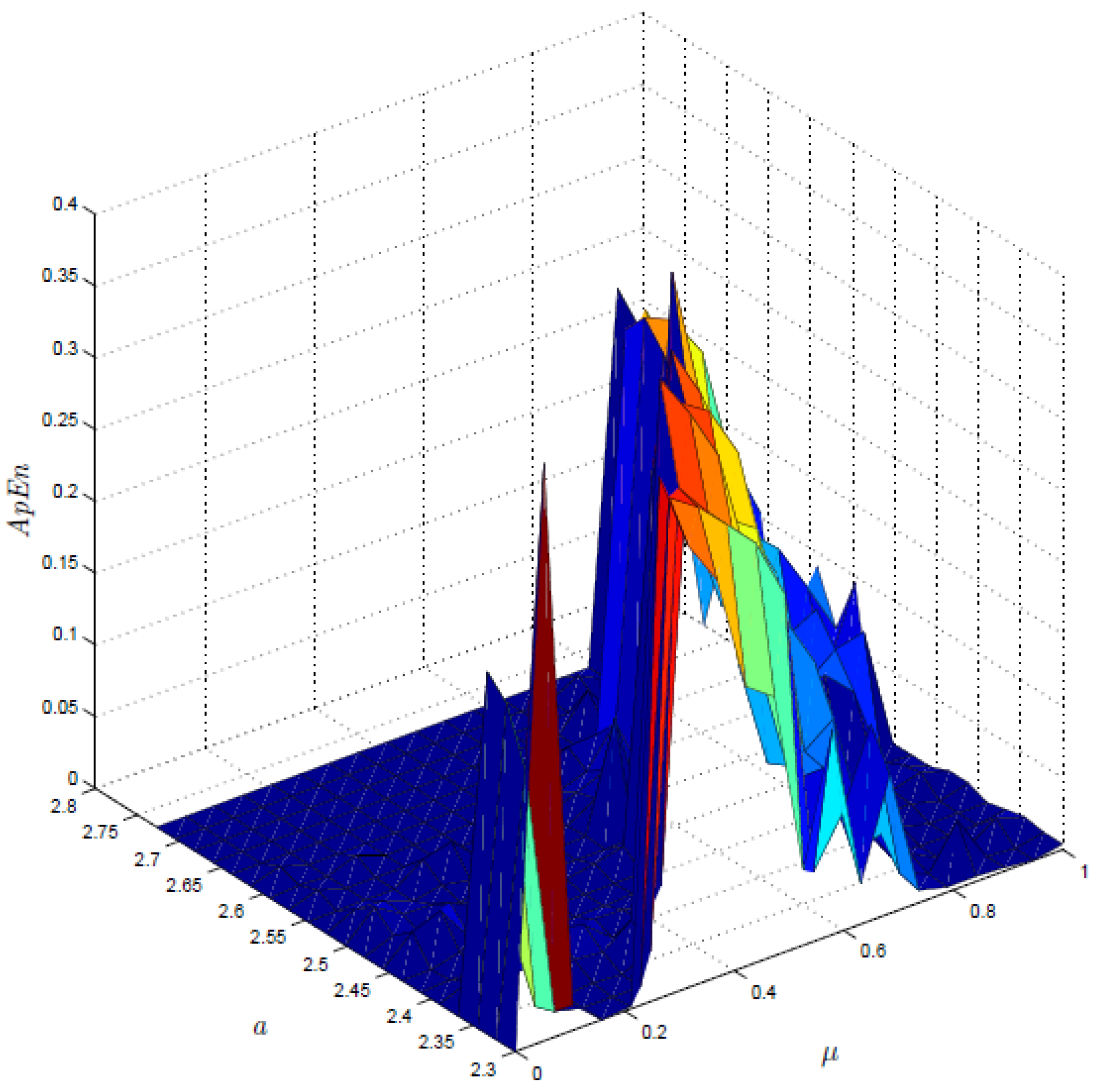
5. Complexity Analysis of the FODTS

In this section, the complexity of the FODTS (3) is analyzed using the approximate entropy (ApEn) [20]. An approximate entropy indicates how complex a system generated by a time series is. In general, a time series with the largest values of ApEn is considered as being more complex. ApEn can be calculated for both continuous and discrete systems and integer and fractional orders. Firstly, the calculating process of the $ApEn$ algorithm is presented [32]. For the specific calculating method, we consider N points of the state ${\left(x_1\right)}_{i=1,..,N}$; the specific steps are as follows:

• Step 1. Construct a sequence of m vectors. For a given time series ${\left(x_1\right)}_{i=1,..,N}$, the m vector sequence $\{X_m\left(1\right),\dots ,X_{i+m-1}\}$ is constructed as

  $$X_m\left(1\right)=\{x\left(i\right),x(i+1),\dots ,x(i+m-1)\},1\le i\le B-m+1.$$
• Step 2. For each $1\le i\le N-m+1$, define the following equation

  $$C_r^m\left(i\right)=\frac{nbrofd\left[X\right(i),X(j\left)\right]\le r}{N-m+1},$$

  where $d\left[X\left(i\right),X\left(j\right)\right]$ is the distance between $X\left(i\right)$ and $X\left(j\right)$ given by

  $$d\left[X\left(i\right),X\left(j\right)\right]=ma{x}_{k=0,\dots ,m}\left|X(i+k-1)-X(j+k-1)\right|,$$

  and $r=0.2std\left(x\right)$ in which $std\left(x\right)$ presents the standard deviation of the data x.
• Step 3. On the basis of $C_r^m$, the average value is denoted to be

  $${\varphi }^m\left(r\right)=\frac{1}{n-m-1}\sum _{i=1}^{n-m+1}log{C}_i^m\left(r\right).$$

  (9)
• Step 4. The $ApEn$ is calculated as follows

  $$ApEn={\varphi }^m\left(r\right)-{\varphi }^{m+1}\left(r\right).$$

  (10)

The $ApEn$ analysis results of the proposed FODT system (3) with varying $\eta$ and A are shown in Figure 12. It can be seen that the proposed system (3) can have a higher complexity with relatively larger parameter values a and fractional order $\eta$. The analysis results in Figure 12 indicate that the $ApEn$ test cannot distinguish chaos and hyperchaos but it can be used as the parameter choice in the practical application.

Figure 12. The approximate entropy ApEn of the FODTS (3) in the three-dimensional space with the variation of system parameter A and fractional order $\eta$, for $B=0.1$.

6. Control Laws

This section deals with the stability analysis of hyperchaotic FODTS (3). It is our first objective to present the theorem below, which is used as the basis for analyzing the stabilization of fractional discrete systems. Next, we perform numerical simulations to demonstrate the effectiveness of the proposed control method.

Theorem 1

([33]). Let $x=0$ be an equilibrium point for the h-fractional discrete system

$${}_h^C{\Delta }_a^{\eta }x\left(s\right)=f\left(s+\eta h,x\left(s+\eta h\right)\right),s{\left(h\mathbb{N}\right)}_{a+\left(1-\eta \right)h}.$$

(11)

Assume that there exists a positive definite and decrescent scalar function $V\left(s,x\left(s\right)\right)$, such that ${}_h^C{\Delta }_a^{\eta }V\left(s,x\left(s\right)\right)\le 0$ Then the zero equilibrium point of the nonlinear h-fractional discrete system is asymptotically stable.

Lemma 1

([33]). For any discrete time $s\in {\left(h\mathbb{N}\right)}_{a+\left(1-\eta \right)h}$, we have

$${}_h^C{\Delta }_a^{\eta }{x}^2\left(s\right)\le 2x{\left(s+\eta h\right)}_h^C{\Delta }_a^{\eta }x\left(s\right),0<\eta \le 1.$$

(12)

To obtain our results, the following theorem is presented.

Theorem 2.

The two-dimensional FODTS (3) is controlled under the following one-dimensional control law

$$\mathbf{C}\left(s\right)=-\left(\left|A\right|+1\right)x_1\left(s\right)-x_2\left(s\right)-B,$$

(13)

where $s\in {\left(h\mathbb{N}\right)}_{a+\left(1-\eta \right)h}$.

Proof. 

The controlled FODTS can be described as

$$\left\{\begin{array}{c}{}^C{\Delta }_a^{\eta }{x}_1\left(s\right)=A{x}_1(s-\eta +1)sin\left(x_2(s-\eta +1)\right)+B+\mathbf{C}(s-\eta +1),\hfill \\ {}^C{\Delta }_a^{\eta }{x}_2\left(s\right)=x_1(s-\eta +1),\hfill \end{array}\right.$$

(14)

Consequently, (14) takes the form:

$$\left\{\begin{array}{c}{}^C{\Delta }_a^{\eta }{x}_1\left(s\right)=A{x}_1(s-\eta +1)sin\left(x_2(s-\eta +1)\right)-\left(\left|A\right|+1\right)x_1(s-\eta +1)-x_2(s-\eta +1),\hfill \\ {}^C{\Delta }_a^{\eta }{x}_2\left(s\right)=x_1(s-\eta +1),\hfill \end{array}\right.$$

(15)

One can utilize the Lyapunov method by first letting the Lyapunov function, $V\left(s\right)$, in the form:

$$V=\frac{1}{2}{x}_1^2\left(s\right)+\frac{1}{2}{x}_1^2\left(s\right),$$

(16)

the adoption of the Caputo h-difference operator implies that

$${}_h^C{\Delta }_a^{\eta }V\left(s\right)=\frac{1}{2}{}_h^C{\Delta }_a^{\eta }{x}_1^2\left(s\right)+\frac{1}{2}{}_h^C{\Delta }_a^{\eta }{x}_2^2\left(s\right).$$

(17)

By using Lemma 1, it follows that

$$\begin{array}{ccc}\hfill {}_h^C{\Delta }_a^{\eta }V& \le & x_1{(s+\eta h)}_h^C{\Delta }_a^{\eta }{x}_1\left(s\right)+x_2{(s+\eta h)}_h^C{\Delta }_a^{\eta }{x}_2\left(s\right)\hfill \\ & =& x_1(s-\eta +1)\left[A{x}_1(s-\eta +1)sin\left(x_2(s-\eta +1)\right)-\left(\left|A\right|+1\right)x_1(s-\eta +1)-x_2(s-\eta +1)\right]\hfill \\ & & x_2(s-\eta +1)x_1(s-\eta +1)\hfill \\ & =& A{x}_1^2(s-\eta +1)sin\left(x_2(s-\eta +1)\right)-\left(\left|A\right|+1\right)x_1^2(s-\eta +1)\hfill \\ & \le & \left|A{x}_1^2(s-\eta +1)sin\left(x_2(s-\eta +1)\right)\right|-\left(\left|A\right|+1\right)x_1^2(s-\eta +1)\hfill \\ & \le & \left|A\right|x_1^2(s-\eta +1)\left|sin\left(x_2(s-\eta +1)\right)\right|-\left(\left|A\right|+1\right)x^2(s-\eta +1)\hfill \\ & \le & \left|A\right|x_1^2(s-\eta +1)-\left(\left|A\right|+1\right)x_1^2(s-\eta +1)\hfill \\ & =& -x_1^2(s-\eta +1)\le 0\hfill \end{array}$$

Theorem 1 states that (14) has an asymptotically stable zero equilibrium. This implies that the chaotic trajectories of this proposed FODTS (3) are stabilized by the linear control law (13).   □

As shown in Section 3, the FODTS (3) with $A=2.8,B=0.1$, and $\eta =0.98$ display chaotic behavior. Figure 13 depicts the evolution of states and the phase space plot of the controlled FODTS (3), respectively. As one can see, the FODTS (3) is completely controlled in a stable state. These plots confirm that the hidden chaotic dynamic of the FODTS is controlled effectively.

Figure 13. Evolution of states and the phase space plot of the controlled FODTS (3) with fractional order $\eta =0.98$ and system parameters $A=2.8,B=0.1$.

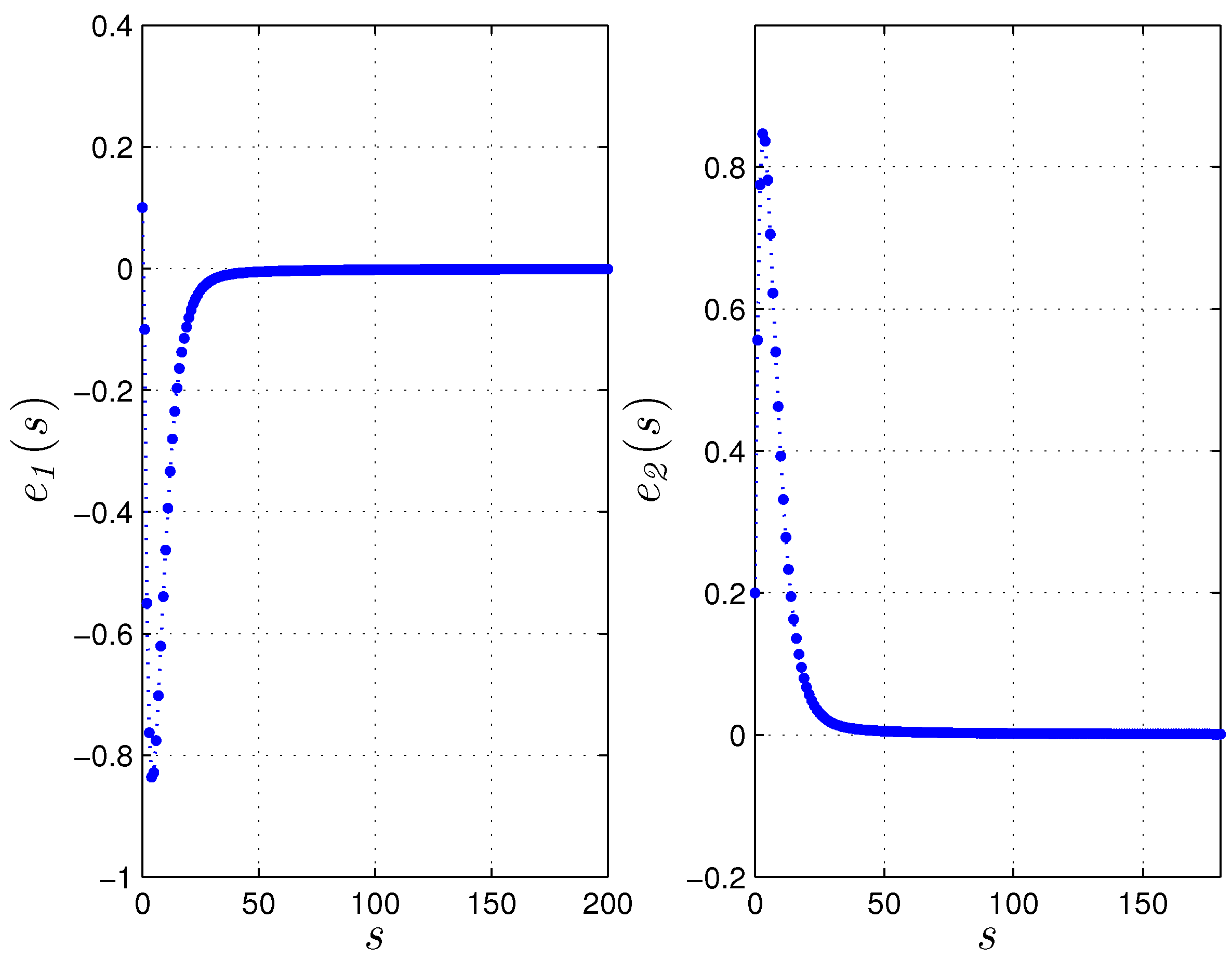
7. Synchronization

In this section, we will investigate the synchronization of the hyperchaotic FODTS (3). We present a new theorem that ensures that the dynamics of two chaotic FODT systems are synchronized through linear control laws of a very simple nature. The master discrete system is defined as

$$\left\{\begin{array}{c}{}^C{\Delta }_a^{\eta }{x}_{1m}\left(s\right)=A{x}_{1m}(s-\eta +1)sin\left(x_{2m}(s-\eta +1)\right)+B,\hfill \\ {}^C{\Delta }_a^{\eta }{x}_{2m}\left(s\right)=x_{1m}(s-\eta +1),\hfill \end{array}\right.$$

(18)

and the slave system as

$$\left\{\begin{array}{c}{}^C{\Delta }_a^{\eta }{x}_{1s}\left(s\right)=A{x}_{1s}(s-\eta +1)sin\left(x_{2s}(s-\eta +1)\right)+B+{\mathbf{L}}_1,\hfill \\ {}^C{\Delta }_a^{\eta }{x}_{2s}\left(s\right)=x_{1s}(s-\eta +1)+{\mathbf{L}}_2,\hfill \end{array}\right.$$

(19)

where ${\mathbf{L}}_1$ and ${\mathbf{L}}_2$ are synchronization controllers that have to be designed. Using the master (18) and slave discrete systems (19), the error dynamics can be derived as

$$\left\{\begin{array}{c}{e}_1=x_{1s}-x_{1m},\hfill \\ e_2=x_{2s}-x_{2m},\hfill \end{array}\right.$$

(20)

If $\underset{s\to +\infty }{lim}\left|e_i\left(s\right)\right|=0$, then the synchronization scheme is achieved.

The following theorem, which we consider as being one of the most important outcomes of this research, is intended to highlight the important results obtained by the proposed synchronization scheme.

Theorem 3.

The master system (18) and the slave system (19) achieve synchronized dynamics, provided that the control law is selected as

$$\left\{\begin{array}{c}{\mathbf{L}}_1\left(s\right)=-\left(\left|A\right|+\frac{{\left(Al\right)}^2}{4}\right)e_1,\hfill \\ {\mathbf{L}}_2\left(s\right)=-e_1-e_2,\hfill \end{array}\right.$$

(21)

where $s\in {\left(h\mathbb{N}\right)}_{a+\left(1-\eta \right)h}.$

Proof. 

To establish an asymptotic convergence of the synchronization errors, given in (20), we start applying the Caputo-type fractional-order differences on (20), which yields:

$$\left\{\begin{array}{c}{}_h^C{\Delta }_a^{\eta }{e}_1=A\left[x_{1s}(s-\eta +1)sin\left(x_{2s}(s-\eta +1)\right)-x_{1s}(s-\eta +1)sin\left(x_{2s}(s-\eta +1)\right)\right]+{\mathbf{L}}_1,\hfill \\ {}_h^C{\Delta }_a^{\eta }{e}_2=x_{1s}(s-\eta +1)-x_{1m}(s-\eta +1)+{\mathbf{L}}_2,\hfill \end{array}\right.$$

(22)

(21) is subsumed into (22) to yield the following new discrete system:

$$\left\{\begin{array}{c}{}_h^C{\Delta }_a^{\eta }{e}_1=A\left[x_{1s}(s-\eta +1)sin\left(x_s(s-\eta +1)\right)-x_{1s}(s-\eta +1)sin\left(x_{2s}(s-\eta +1)\right)\right]-\left(\left|A\right|+\frac{{\left(Al\right)}^2}{4}\right)e_1,\hfill \\ {}_h^C{\Delta }_a^{\eta }{e}_2=-e_2,\hfill \end{array}\right.$$

(23)

Let $V=\frac{1}{2}{e}_1^2\left(s\right)+\frac{1}{2}{e}_2^2\left(s\right).$ This implies ${}^C{\Delta }_a^{\eta }V=$${}^C{\Delta }_a^{\eta }{e}_1^2\left(s\right)+$${}^C{\Delta }_a^{\eta }{e}_2^2\left(s\right),$ and by using Lemma 1, we obtain

$$\begin{array}{ccc}\hfill {}^C{\Delta }_a^{\eta }V& \le & e_1{(s-\eta +1)}^C{\Delta }_a^{\eta }{e}_1(s-\eta +1)+e_2{(s-\eta +1)}^C{\Delta }_a^{\eta }{e}_2(s-\eta +1)\hfill \\ & =& a{e}_1(t-\eta +1)\left[x_{1s}(s-\eta +1)sin\left(x_{2s}(s-\eta +1)\right)-x_{1s}(s-\eta +1)sin\left(x_{2s}(s-\eta +1)\right)\right]\hfill \\ & & -\left(\left|A\right|+\frac{{\left(Al\right)}^2}{4}\right)e_1^2-e_2^2(s-\eta +1)\hfill \end{array}$$

one can write:

$$\begin{array}{cc}& x_{1s}(s-\eta +1)sin\left(x_{2s}(s-\eta +1)\right)-x_{1s}(s-\eta +1)sin\left(x_{2s}(s-\eta +1)\right)\\ & =x_{1s}(s-\eta +1)\left(sin\left(x_{2s}(s-\eta +1)\right)-sin\left(x_{2m}(s-\eta +1)\right)\right)\\ & -\left(x_{1s}(s-\eta +1)-x_{1m}(s-\eta +1)\right)sin\left(x_{2m}(s-\eta +1)\right)\end{array}$$

So, we have

$$\begin{array}{ccc}\hfill {}^C{\Delta }_a^{\eta }V& \le & \left|A\right|\left|e_1(t-\eta +1)\right|\left|x_{1s}(s-\eta +1)\right|\left|\left(sin\left(x_{2s}(s-\eta +1)\right)-sin\left(x_{2m}(s-\eta +1)\right)\right)\right|\hfill \\ & & +\left|A\right|e_1^2(s-\eta +1)\left|sin\left(x_{2m}(s-\eta +1)\right)\right|-\left(\left|A\right|+\frac{{\left(A\right)}^2}{4}\right)e_1^2-e_2^2(s-\eta +1)\hfill \end{array}$$

since fractional chaotic maps have the ‘property of boundedness’, we can put

$$\left|x_{1s}(s-\eta +1)\right|\le l$$

and

$$\left|\left(sin\left(x_{2s}(s-\eta +1)\right)-sin\left(x_{2m}(s-\eta +1)\right)\right)\right|\le \left|x_{2s}(s-\eta +1)-x_{2m}(s-\eta +1)\right|$$

so we have

$$\begin{array}{ccc}\hfill {}^C{\Delta }_a^{\eta }V& \le & \left|A\right|l\left|e_1(s-\eta +1)\right|\left|\left(x_{2s}(s-\eta +1)-x_{2m}(s-\eta +1)\right)\right|+\left|A\right|e_1^2(s-\eta +1)\hfill \\ & & -\left(\left|A\right|+\frac{{\left(Al\right)}^2}{4}\right)e_1^2-e_2^2(s-\eta +1)\hfill \\ & =& \left|A\right|l\left|e_1(s-\eta +1)\right|\left|e_2(s-\eta +1)\right|-\frac{{\left(A\right)}^2}{4}{e}_1^2-e_2^2(s-\eta +1)\hfill \\ & =& -{\left(\frac{\left|A\right|l}{2}{e}_1-e_2\right)}^2<0.\hfill \end{array}$$

According to the stability theorem (Theorem 1), error system (22) is stabilized to the origin. This means that the fractional slave discrete system (19) can asymptotically synchronize the fractional master discrete system (18).   □

The synchronization errors between the hyperchaotic FODT master and slave systems are depicted in Figure 14 for the initial values $e_1\left(0\right)=1,e_2\left(0\right)=-2,$ and $\eta =0.98$. There is a convergence of errors into zero, which indicates that chaos synchronization has indeed been achieved.

Figure 14. Evolution of synchronization error states with FODTS $\eta =0.98$ and system parameters $A=2.8,B=0.1$.

8. Conclusions

A 2D fractional map with hidden multistability is presented using the Caputo-like difference operator. Bifurcation diagrams, Lyapunov exponents, and phase portraits have been used to study the dynamics of the system in detail. Multiple hidden attractors have been revealed in the new fractional map. In order to stabilize the chaotic trajectories of the fractional discrete-time system, a new theorem has been illustrated. A new theorem assures that two hyperchaotic fractional discrete-time systems can achieve synchronized dynamics via very simple linear control laws. Future work will involve leveraging the hardware implementation developed herein in order to develop cryptographic applications based on fractional maps with hidden chaotic attractors. It is being investigated how fractional maps with hidden attractors can be used to develop new types of fractional pseudo-number generators.

References

- Herrmann, R. Fractional Calculus—An Introduction for Physicists; World Scientific: Singapore, 2018. [Google Scholar]
- Diaz, J.B.; Olser, T.J. Differences of fractional order. Math. Comput. 1974, 28, 185–202. [Google Scholar] [CrossRef] [Green Version]
- Goodrich, C.; Peterson, A.C. Discrete Fractional Calculus; Springer: Berlin/Heidelberg, Germany, 2015. [Google Scholar]
- Zaslavsky, G.M.; Zaslavskij, G.M. Hamiltonian Chaos and Fractional Dynamics; Oxford University Press: Oxford, UK, 2005. [Google Scholar]
- Wang, Y.; Liu, S.; Li, H. On fractional difference logistic maps: Dynamic analysis and synchronous control. Nonlinear Dyn. 2020, 102, 579–588. [Google Scholar] [CrossRef]
- Kassim, S.; Hamiche, H.; Djennoune, S.; Bettayeb, M. A novel secure image transmission scheme based on synchronization of fractional-order discrete-time hyperchaotic systems. Nonlinear Dyn. 2017, 88, 2473–2489. [Google Scholar] [CrossRef]
- Khennaoui, A.A.; Ouannas, A.; Bendoukha, S.; Grassi, G.; Lozi, R.P.; Pham, V.T. On fractional–order discrete–time systems: Chaos, stabilization and synchronization. Chaos Solitons Fractals 2019, 119, 150–162. [Google Scholar] [CrossRef]
- Wu, G.C.; Baleanu, D. Discrete fractional logistic map and its chaos. Nonlinear Dyn. 2014, 75, 283–287. [Google Scholar] [CrossRef]
- Alpar, O. Dynamics of a new generalized fractional one-dimensional map: Quasiperiodic to chaotic. Nonlinear Dyn. 2018, 94, 1377–1390. [Google Scholar] [CrossRef]
- Khennaoui, A.A.; Ouannas, A.; Bendoukha, S.; Grassi, G.; Wang, X.; Pham, V.T.; Alsaadi, F.E. Chaos, control, and synchronization in some fractional-order difference equations. Adv. Differ. Equ. 2019, 1, 1–23. [Google Scholar] [CrossRef] [Green Version]
- Peng, Y.; Sun, K.; Peng, D.; Ai, W. Dynamics of a higher dimensional fractional-order chaotic map. Phys. A Stat. Mech. Its Appl. 2019, 525, 96–107. [Google Scholar] [CrossRef]
- Wang, L.; Sun, K.; Peng, Y.; He, S. Chaos and complexity in a fractional-order higher-dimensional multi-cavity chaotic map. Chaos Solitons Fractals 2020, 131, 109488. [Google Scholar] [CrossRef]
- Rong, K.; Bao, H.; Li, H.; Hua, Z.; Bao, B. Memristive Hénon map with hidden Neimark-Sacker bifurcations. Nonlinear Dyn. 2022, 108, 4459–4470. [Google Scholar] [CrossRef]
- Bao, H.; Li, H.; Hua, Z.; Xu, Q.; Bao, B.C. Sine Transform-Based Memristive Hyperchaotic Model with Hardware Implementation. IEEE Trans. Ind. Inform. 2022; in press. [Google Scholar] [CrossRef]
- Li, K.; Bao, H.; Li, H.; Ma, J.; Hua, Z.; Bao, B. Memristive Rulkove neuron model with magnetic inclution effects. IEEE Trans. Ind. Inform. 2021, 18, 1726–1736. [Google Scholar] [CrossRef]
- Bao, H.; Hua, Z.; Li, H.; Chen, M.; Bao, B. Discrete memristor hyperchaotic maps. IEEE Trans. Circuits Syst. Regul. Pap. 2021, 68, 4534–4544. [Google Scholar] [CrossRef]
- Hadjabi, F.; Ouannas, A.; Shawagfeh, N.; Khennaoui, A.A.; Grassi, G. On Two-Dimensional Fractional Chaotic Maps with Symmetries. Symmetry 2020, 12, 756. [Google Scholar] [CrossRef]
- Liu, T.; Mou, J.; Banerjee, S.; Cao, Y.; Han, X. A new fractional-order discrete BVP oscillator model with coexisting chaos and hyperchaos. Nonlinear Dyn. 2021, 106, 1011–1026. [Google Scholar] [CrossRef]
- Amatroud, A.O.; Khennaoui, A.A.; Ouannas, A.; Pham, V.T. Infinite Line of Equilibrium in a Novel Fractional Map with Coexisting Attractors and Initial Offset Boosting. Available online: https://www.degruyter.com/document/doi/10.1515/ijnsns-2020-0180/pdf (accessed on 5 December 2022).
- Pincus, S.M. Approximate entropy as a measure of system complexity. Proc. Natl. Acad. Sci. USA 1991, 88, 2297–2301. [Google Scholar] [CrossRef] [Green Version]
- Ouannas, A.; Khennaoui, A.A.; Momani, S.; Grassi, G.; Pham, V.T. Chaos and control of a three-dimensional fractional order discrete-time system with no equilibrium and its synchronization. AIP Adv. 2020, 10, 045310. [Google Scholar] [CrossRef]
- Ouannas, A.; Bendoukha, S. Generalized and inverse generalized synchronization of fractional–order discrete–time chaotic systems with non–identical dimensions. Adv. Differ. Equ. 2018, 2018, 303. [Google Scholar] [CrossRef]
- Bendoukha, S.; Ouannas, A.; Wang, X.; Khennaoui, A.A.; Pham, V.T.; Grassi, G.; Huynh, V.V. The co-existence of different synchronization types in fractional-order discrete-time chaotic systems with non–identical dimensions and orders. Entropy 2018, 20, 710. [Google Scholar] [CrossRef] [Green Version]
- Ouannas, A.; Khennaoui, A.A.; Zehrour, O.; Bendoukha, S.; Grassi, G.; Pham, V.T. Synchronisation of integer-order and fractional-order discrete-time chaotic systems. Pramana 2019, 92, 52. [Google Scholar] [CrossRef]
- Bao, B.C.; Li, H.Z.; Zhu, L.; Zhang, X.; Chen, M. Initial-switched boosting bifurcations in 2D hyperchaotic map. Chaos Interdiscip. J. Nonlinear Sci. 2020, 30, 033107. [Google Scholar] [CrossRef]
- Khennaoui, A.A.; Almatroud, A.O.; Ouannas, A.; Al-sawalha, M.M.; Grassi, G.; Pham, V.T.; Batiha, I.M. An Unprecedented 2-Dimensional Discrete-Time Fractional-Order System and Its Hidden Chaotic Attractors. Math. Probl. Eng. 2021, 2021, 6768215. [Google Scholar] [CrossRef]
- Wu, G.C.; Baleanu, D. Jacobian matrix algorithm for Lyapunov exponents of the discrete fractional maps. Commun. Nonlinear Sci. Numer. Simul. 2015, 22, 95–100. [Google Scholar] [CrossRef]
- Zhang, S.; Zeng, J.; Wang, X.; Zeng, Z. A novel no-equilibruim HR neuron model with hidden homogeneous extreme multistability. Chaos Solitons Frractals 2021, 145, 11761. [Google Scholar]
- Li, C.; Sprott, J.C. Finding coexisting attractors using amplitude control. Nonlinear Dyn. 2014, 780, 2059–2064. [Google Scholar] [CrossRef]
- Leutcho, G.D.; Wang, H.; Kengne, R.; Kengne, L.K.; Njitacke, Z.T.; Fozin, T.F. Symmetry breaking amplitude control and constant Lyapunov exponent based on single parameter snap flows. Eur. Phys. J. Spec. Top. 2021, 230, 1887–1903. [Google Scholar] [CrossRef]
- Viayajumar, M.D.; Natiq, H.; Leutcho, G.D.; Rajagopal, K.; Jafri, S.; Hussain, I. Hidden and self-Excited Collective Dynamics of a New Multistable Hyper-Jerk System with Unique Equilibrium. Int. J. Bifurc. Chaos 2022, 32, 2250063. [Google Scholar] [CrossRef]
- Cafagna, D.; Grassi, G. An effective method for detecting chaos in fractional-order systems. Int. J. Bifurc. Chaos 2010, 20, 669–678. [Google Scholar] [CrossRef]
- Baleanu, D.; Wu, G.C.; Bai, Y.R.; Chen, F.L. Stability analysis of Caputoâ like discrete fractional systems. Commun. Nonlinear Sci. Numer. Simul. 2017, 48, 520–530. [Google Scholar] [CrossRef]
Disclaimer/Publisher’s Note: The statements, opinions and data contained in all publications are solely those of the individual author(s) and contributor(s) and not of MDPI and/or the editor(s). MDPI and/or the editor(s) disclaim responsibility for any injury to people or property resulting from any ideas, methods, instructions or products referred to in the content. |
© 2023 by the authors. Licensee MDPI, Basel, Switzerland. This article is an open access article distributed under the terms and conditions of the Creative Commons Attribution (CC BY) license (https://creativecommons.org/licenses/by/4.0/).
Share and Cite
Khennaoui, A.-A.; Ouannas, A.; Bekiros, S.; Aly, A.A.; Alotaibi, A.; Jahanshahi, H.; Alsubaie, H. Hidden Homogeneous Extreme Multistability of a Fractional-Order Hyperchaotic Discrete-Time System: Chaos, Initial Offset Boosting, Amplitude Control, Control, and Synchronization. Symmetry 2023, 15, 139. https://doi.org/10.3390/sym15010139
Khennaoui A-A, Ouannas A, Bekiros S, Aly AA, Alotaibi A, Jahanshahi H, Alsubaie H. Hidden Homogeneous Extreme Multistability of a Fractional-Order Hyperchaotic Discrete-Time System: Chaos, Initial Offset Boosting, Amplitude Control, Control, and Synchronization. Symmetry. 2023; 15(1):139. https://doi.org/10.3390/sym15010139
Chicago/Turabian StyleKhennaoui, Amina-Aicha, Adel Ouannas, Stelios Bekiros, Ayman A. Aly, Ahmed Alotaibi, Hadi Jahanshahi, and Hajid Alsubaie. 2023. "Hidden Homogeneous Extreme Multistability of a Fractional-Order Hyperchaotic Discrete-Time System: Chaos, Initial Offset Boosting, Amplitude Control, Control, and Synchronization" Symmetry 15, no. 1: 139. https://doi.org/10.3390/sym15010139