
Investigating the Impact of Fractional Non-Linearity in the Klein–Fock–Gordon Equation on Quantum Dynamics
by
 , , ,
, , ,
Saima Noor
1,*,
Azzh Saad Alshehry
2,
Noufe H. Aljahdaly
3,
Hina M. Dutt
4,*,
Imran Khan
5 and
Rasool Shah
5 1
Department of Basic Sciences, Preparatory Year Deanship, King Faisal University, Al Ahsa 31982, Saudi Arabia
2
Department of Mathematical Sciences, Faculty of Sciences, Princess Nourah Bint Abdulrahman University, P.O. Box 84428, Riyadh 11671, Saudi Arabia
3
Department of Mathematics, Faculty of Sciences and Arts, King Abdulaziz University, Rabigh 21911, Saudi Arabia
4
Department of Humanities and Sciences, School of Electrical Engineering and Computer Science (SEECS), National University of Sciences and Technology (NUST), Islamabad 44000, Pakistan
5
Department of Mathematics, Abdul Wali Khan University, Mardan 23200, Pakistan
*
Authors to whom correspondence should be addressed.
Symmetry 2023, 15(4), 881; https://doi.org/10.3390/sym15040881
Submission received: 13 March 2023
/
Revised: 4 April 2023
/
Accepted: 5 April 2023
/
Published: 7 April 2023
(This article belongs to the Special Issue Symmetry in Quantum Calculus)
Abstract
:In this paper, we investigate the fractional-order Klein–Fock–Gordon equations on quantum dynamics using a new iterative method and residual power series method based on the Caputo operator. The fractional-order Klein–Fock–Gordon equation is a generalization of the traditional Klein–Fock–Gordon equation that allows for non-integer orders of differentiation. This equation has been used in the study of quantum dynamics to model the behavior of particles with fractional spin. The Laplace transform is employed to transform the equations into a simpler form, and the resulting equations are then solved using the proposed methods. The accuracy and efficiency of the method are demonstrated through numerical simulations, which show that the method is superior to existing numerical methods in terms of accuracy and computational time. The proposed method is applicable to a wide range of fractional-order differential equations, and it is expected to find applications in various areas of science and engineering.
1. Introduction
Fractional calculus (FC), which has existed since classical calculus, has recently received much interest due to its connections to basic ideas. Leibniz and L’Hospital were the first to present fractional calculus, but it has since gained popularity among academics due to its wide range of applications. Following that, it was widely used to examine a variety of occurrences. However, several types of research emphasized the disadvantages of using this operator, specifically the physical importance of the starting condition and the derivative of a non-zero constant. Then, Caputo introduced a novel fractional operator that overcame the earlier limitations. Most models explored and analyzed under the FC framework use the Caputo operator. Momani and Shawagfeh provide several basic works of fractional calculus on various aspects [1]: Podlubny [2], Jafari and Seifi [3,4], Kiryakova [5], Oldham and Spanier [6], Miller and Ross [7], Diethelm et al. [8], Trujillo [9], Kilbas and Kemple and Beyer [10] and so on [11,12,13].
The Klein–Fock–Gordon equation is related to quantum dynamics because it describes the time evolution of the wave function of a relativistic particle. The wave function contains all the information about the particle’s position, momentum, and other physical properties. The solutions of the Klein–Fock–Gordon equation are used to calculate the probabilities of different outcomes of measurements on the particle [14,15,16,17,18]. These probabilities are related to the behavior of the wave function over time, as governed by the equation. The Klein–Fock–Gordon equation is a fundamental equation in quantum dynamics that describes the behavior of spin-zero particles in the context of special relativity. Its solutions provide information about the probabilities of different outcomes of measurements on these particles [19,20,21,22].
The connection between symmetry and the Klein–Gordon equation is also of great interest. The Klein–Gordon equation is invariant under the Lorentz transformation, a symmetry transformation that preserves the speed of light and the space–time interval. This symmetry is related to the special theory of relativity and has important consequences for the behavior of particles in high-energy physics [23,24,25,26]. In addition, the Klein–Gordon equation can exhibit other symmetries, such as gauge symmetry and super symmetry. Gauge symmetry is a local symmetry related to particle behavior under electromagnetic and other gauge interactions. Super symmetry is a symmetry that relates particles with different spins and has important implications for studying fundamental particles. In summary, investigating the impact of fractional non-linearity in the Klein–Gordon equation on quantum dynamics and the connection between symmetry is an active area of research that has important implications for theoretical and experimental physics [27,28,29,30,31].
The Klein–Fock–Gordon (KFG) equation is a fundamental quantum mechanics equation that describes spinless particles’ behavior in relativistic settings. It is named after the physicists Klein, Fock, and Gordon, who developed the equation. The KFG equation, known as the relativistic wave equation, is a quantized form of the relationship between relativistic energy and momentum. It is closely related to the Schrodinger equation and is used to describe relativistic electrons. However, the classical Klein–Fock–Gordon equation has limitations in describing the dynamics of some physical systems, such as viscoelastic materials and biological systems, which exhibit non-local and memory effects. To overcome these limitations, researchers have proposed using fractional calculus to generalize the Klein–Fock–Gordon equation, resulting in the fractional-order Klein–Fock–Gordon equation.
The fractional-order Klein–Fock–Gordon equation is a partial differential equation that incorporates fractional derivatives, which are non-local operators that describe a system’s memory and hereditary effects. These derivatives offer a more precise depiction of the actions of viscoelastic materials, biological systems, and other physical systems. This equation has attracted significant attention from researchers due to its potential applications in many areas, including nanotechnology, condensed-matter physics, and medical imaging. Moreover, studying the fractional-order Klein–Fock–Gordon equation has also led to the development of new mathematical tools and techniques, which can be used to solve other problems in fractional calculus and quantum mechanics.
In this context, this paper aims to provide an overview of the fractional-order Klein–Fock–Gordon equation and its application to quantum dynamics. We discuss the mathematical framework of the equation, its physical interpretation, and its properties. Furthermore, we review recent research on the numerical methods used to solve this equation and its applications to various physical systems. Overall, this paper comprehensively reviews the fractional-order Klein–Fock–Gordon equation and its role in quantum dynamics. The following fractional-order Klein–Fock–Gordon equation is taken into consideration in this article as:
along with initial conditions: and . The Klein–Fock–Gordon equation, with n being a positive integer and being real constants, has appeared in various physical phenomena, including non-linear optics, quantum field theory, the interaction of solitons in collisionless plasma, and condensed-matter physics. The KFG equation has been studied by different methods, such as the homotopy analysis method [32], variational iteration method [33], modified differential transform method [34], differential transform method [35], q-homotopy analysis transform method [36], and homotopy analysis transform method [37].
The residual power series method (RPSM), a powerful and simple approach for determining the coefficients of power series solutions for first- and second-order fuzzy differential equations, was developed by Jordanian mathematician Omar Abu Arqub in 2013. Unlike other techniques, the RPSM does not necessitate perturbation, linearization, or discretization and can provide effective solutions for both linear and non-linear equations [38,39,40]. In recent years, the method has been applied to solve a wide range of non-linear ordinary and partial differential equations of various orders and classes [41,42,43,44,45]. The RPSM has been applied in several areas, including the prediction of solitary patterns in non-linear fractional dispersive partial differential equations, the resolution of the highly non-linear singular differential equation known as the generalized Lane–Emden equation, and the approximation of the solution to fractional non-linear KdV–Burger equations [46,47].
Compared to other analytical and numerical approaches, the RPSM has some distinct advantages. Firstly, it does not require a recursion connection or the comparison of coefficients of related terms. Secondly, it offers a straightforward way to ensure the convergence of the series solution by reducing the associated residual error. Thirdly, it does not suffer from computational rounding errors and does not require much time or memory [48,49,50]. Lastly, the RPSM can be directly applied to a specific issue by selecting a suitable initial approximation and does not necessitate any transformations when shifting from low-order to high-order or from simple linearity to complex non-linearity [51,52,53].
The structure of this work is organized as follows: Section 2 covers fundamental aspects of calculus theory. Section 3 and Section 4 present the RPSTM and NITM formulations used to derive the general solution. To demonstrate the effectiveness and feasibility of both approaches, Section 5 includes numerical examples and comparisons to the exact solution. The conclusion is provided in Section 6.
2. Fundamental Definitions
Definition 1.
The fractional Caputo derivative of the function of order ρ is expressed as [54]
where and are the fractional integral Riemann–Liouville of of the fractional-order ρ, which is defined as
supposing that the provided integral exists.
Definition 2.
The Laplace transformation of the term is defined as [54]
where the inverse Laplace transform is defined as
Lemma 1.
Suppose that is piecewise continuous term and of exponential-order ζ and , we obtain
- 1.
- .
- 2.
- .
- 3.
- .
Proof.
For proof, see Ref. [54]. □
Theorem 1.
Let be a function that is piecewise continuous on the interval and has an exponential order of ζ. Assuming that the function has a fractional expansion, we have:
Then, .
Proof.
For proof, see Ref. [54]. □
3. Road Map of RPSTM
In this section, we show the general methodology LRPS method for the fractional-order partial differential equations
and consider the following IC’s:
Applying the LT of Equation (6) and making use of (7), we obtain
Suppose that the result of Equation (8) has the following
The -truncated term series are
The Laplace residual functions are
Furthermore, the -LRFs are:
Some characteristics arising in the RPSTM are given as:
- and for each
- .
To find the coefficients , we recursively solve the following system
Finally, we apply inverse Laplace transform to Equation (11) to achieve the analytic solution of .
4. Basic Idea of New Iterative Method
To explain the fundamental concept of the new iterative method, we examine the general functional equation:
Here, N is a non-linear operator from a Banach space B to B, and f is an unknown function. We seek a solution to Equation (14) in the form of a series:
The non-linear term can be decomposed as
From Equations (15) and (16), Equation (14) is equivalent to
We define the following recurrence relation:
Then,
5. Numerical Problem
In Figure 1, show that the comparison of NIM and LRPSM solution of Problem 1. Figure 2, two-dimensional comparison of NIM and LRPSM solution for at different values of , , and , and . In Figure 3, show that the three dimensional graph of NIM and LRPSM solution of Problem 1. In Table 1, compare the solutions obtained using the proposed technique and the exact method for various fractional orders with of Problem 1.
Problem 1.
Consider that the non-linear FKFG equation is given as
along with the initial conditions:
- Solution by LRPSM
Applying LT to Equation (20) and making use of Equation (21), we obtain
and so the -truncated term series for Equation (33)
and the -LRFs is provided as:
The first few terms are obtained by substituting the -truncate series Equation (23) into the -Laplace residual function Equation (24), multiplying the resulting equation by , and then recursively solving the relation , to determine for .
and so on.
Now, putting the values of , in Equation (23), we obtain
Using the inverse Laplace transform, we obtain
- Solution by NIM
and using the algorithm (18) of Nim we obtain
and the third-order solution using the new iterative method
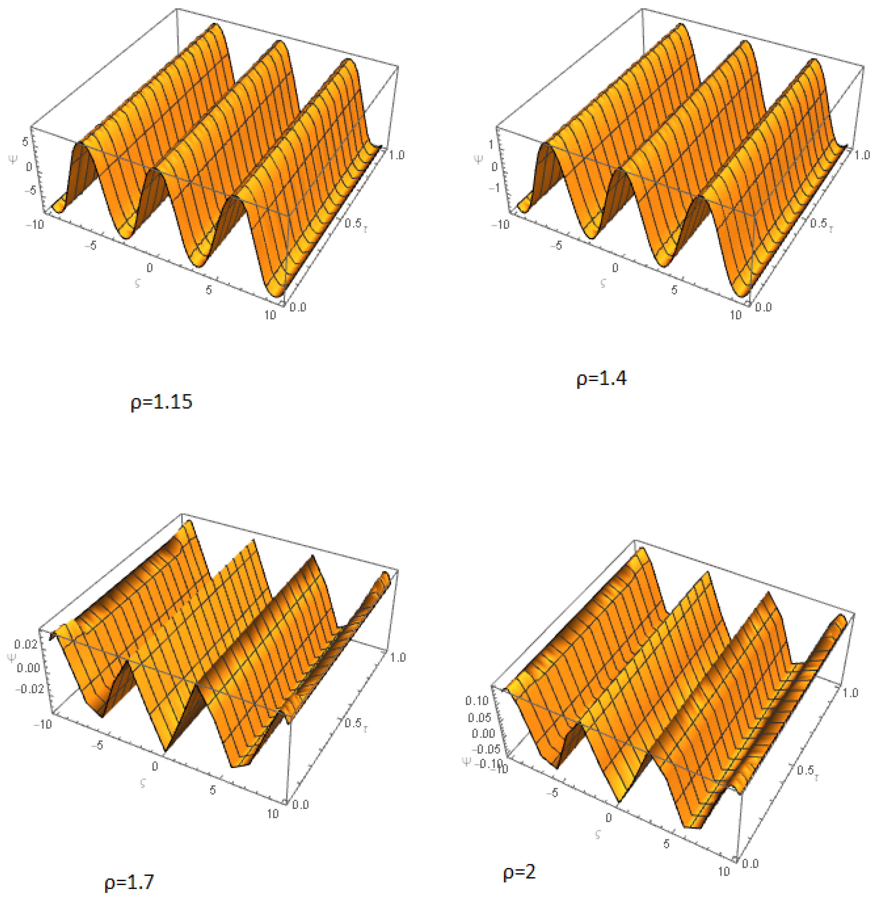
Figure 4, two-dimensional comparison of NIM and LRPSM solution for at different values of , , and , and of Problem 2. In Figure 5, show that the three dimensional graph of NIM and LRPSM solution of Problem 2. In Table 2, compare the solutions obtained using the proposed technique and the exact method for various fractional orders with of Problem 2.
Problem 2.
- Solution by LRPSM
Applying LT to Equation (31) and making use of Equation (32), we obtain
and so the -truncated term series are
and the -LRFs are:
To determine for , we substitute the -truncated series Equation (34) into the -Laplace residual function Equation (35), multiply the resulting equation by , and then recursively solve the relation for . The first few terms are as follows:
Now, putting the values of , in Equation (34), we obtain
Using inverse Laplace transform, we obtain:
- Solution by NIM
6. Conclusions
This paper presents a robust analysis of fractional-order non-linear Klein–Fock–Gordon equations using two powerful analytic methods. The obtained analytical results have been rigorously calculated to confirm the reliability and validity of the suggested techniques. The figures demonstrate a remarkable correlation between the obtained and actual solutions, providing strong evidence to validate and test the accuracy of the proposed methods. Notably, our approaches offer a highly efficient and practical means to address a wide range of non-linear systems involving fractional-order partial differential equations. Furthermore, the substantial reduction in computational requirements further enhances the broad applicability of our methods. These findings highlight the remarkable accuracy of our proposed techniques, which are shown to closely match the actual answers and outperform existing methodologies. Hence, our suggested approaches represent an effective and powerful strategy to solve complex fractional-order partial differential equation non-linear systems.
Author Contributions
Data curation, H.M.D.; Formal analysis, I.K.; Methodology, S.N., A.S.A. and R.S.; Resources, I.K.; Software, S.N., N.H.A. and H.M.D.; Validation, N.H.A. All authors have read and agreed to the published version of the manuscript.
Funding
Princess Nourah bint Abdulrahman University Researchers Supporting Project number (PNURSP2023R183), Princess Nourah bint Abdulrahman University, Riyadh, Saudi Arabia. This work was supported by the Deanship of Scientific Research, the Vice Presidency for Graduate Studies and Scientific Research, King Faisal University, Saudi Arabia (Grant No. 3216).
Data Availability Statement
Data sharing is not applicable to this article as no new data were created or analyzed in this study.
Acknowledgments
Princess Nourah bint Abdulrahman University Researchers Supporting Project number (PNURSP2023R183), Princess Nourah bint Abdulrahman University, Riyadh, Saudi Arabia. This work was supported by the Deanship of Scientific Research, the Vice Presidency for Graduate Studies and Scientific Research, King Faisal University, Saudi Arabia (Grant No. 3216).
Conflicts of Interest
The authors declare no conflict of interest.
References
- Momani, S.; Shawagfeh, N.T. Decomposition method for solving fractional Riccati differential equations. Appl. Math. Comput. 2006, 182, 1083–1092. [Google Scholar] [CrossRef]
- Podlubny, I. Fractional Differential Equations: An introduction to Fractional Derivatives, Fractional Differential Equations, to Methods of Their Solution and Some of Their Applications; Academic Press: New York, NY, USA, 1999. [Google Scholar]
- Jafari, H.; Seifi, S. Homotopy Analysis Method for solving linear and nonlinear fractional diffusion-wave equation. Commun. Nonlinear. Sci. Numer. Simul. 2009, 14, 2006–2012. [Google Scholar] [CrossRef]
- Izadi, M.; Srivastava, H.M. A discretization approach for the nonlinear fractional logistic equation. Entropy 2020, 22, 1328. [Google Scholar] [CrossRef] [PubMed]
- Kiryakova, S.V. Multiple (multiindex) Mittag–Leffler functions and relations to generalized fractional calculus. J. Comput. Appl. Math. 2000, 118, 441–452. [Google Scholar] [CrossRef] [Green Version]
- Oldham, K.B.; Spanier, J. The Fractional Calculus; Academic Press: New York, NY, USA, 1974. [Google Scholar]
- Pitolli, F.; Sorgentone, C.; Pellegrino, E. Approximation of the Riesz-Caputo derivative by cubic splines. Algorithms 2022, 15, 69. [Google Scholar] [CrossRef]
- Diethelm, K.; Ford, N.J.; Freed, A.D. A predictor-corrector approach for the numerical solution of fractional differential equation. Nonlinear Dyn. 2002, 29, 3–22. [Google Scholar] [CrossRef]
- Kilbas, A.A.; Trujillo, J.J. Differential equations of fractional order: Methods, results problems. Appl. Anal. 2001, 78, 153–192. [Google Scholar] [CrossRef]
- Kemple, S.; Beyer, H. Global and Causal Solutions of Fractional Differential Equations, Transform Methods and Special Functions: Varna 96. In Proceedings of the 2nd International Workshop (SCTP), Singapore, 23–30 August 1996; Volume 96, pp. 210–216. [Google Scholar]
- Li, X.; Dong, Z.; Wang, L.; Niu, X.; Yamaguchi, H.; Li, D.; Yu, P. A magnetic field coupling fractional step lattice Boltzmann model for the complex interfacial behavior in magnetic multiphase flows. Appl. Math. Model. 2023, 117, 219–250. [Google Scholar] [CrossRef]
- Sun, L.; Hou, J.; Xing, C.; Fang, Z. A Robust Hammerstein-Wiener Model Identification Method for Highly Nonlinear Systems. Processes 2022, 10, 2664. [Google Scholar] [CrossRef]
- Xu, S.; Dai, H.; Feng, L.; Chen, H.; Chai, Y.; Zheng, W.X. Fault Estimation for Switched Interconnected Nonlinear Systems with External Disturbances via Variable Weighted Iterative Learning. IEEE Trans. Circuits Syst. II Express Briefs 2023. [Google Scholar] [CrossRef]
- Guo, F.; Zhou, W.; Lu, Q.; Zhang, C. Path extension similarity link prediction method based on matrix algebra in directed networks. Comput. Commun. 2022, 187, 83–92. [Google Scholar] [CrossRef]
- Liu, Y.; Xu, K.; Li, J.; Guo, Y.; Zhang, A.; Chen, Q. Millimeter-Wave E-Plane Waveguide Bandpass Filters Based on Spoof Surface Plasmon Polaritons. IEEE Trans. Microw. Theory Tech. 2022, 70, 4399–4409. [Google Scholar] [CrossRef]
- Xu, K.; Guo, Y.; Liu, Y.; Deng, X.; Chen, Q.; Ma, Z. 60-GHz Compact Dual-Mode On-Chip Bandpass Filter Using GaAs Technology. IEEE Electron Device Lett. 2021, 42, 1120–1123. [Google Scholar] [CrossRef]
- Dai, B.; Zhang, B.; Niu, Z.; Feng, Y.; Liu, Y.; Fan, Y. A novel ultrawideband branch waveguide coupler with low amplitude imbalance. IEEE Trans. Microw. Theory Tech. 2022, 70, 3838–3846. [Google Scholar] [CrossRef]
- Feng, Y.; Zhang, B.; Liu, Y.; Niu, Z.; Fan, Y.; Chen, X. A D-Band Manifold Triplexer with High Isolation Utilizing Novel Waveguide Dual-Mode Filters. IEEE Trans. Terahertz Sci. Technol. 2022, 12, 678–681. [Google Scholar] [CrossRef]
- Naeem, M.; Yasmin, H.; Shah, N.A.; Nonlaopon, K. Investigation of Fractional Nonlinear Regularized Long-Wave Models via Novel Techniques. Symmetry 2023, 15, 220. [Google Scholar] [CrossRef]
- Naeem, M.; Yasmin, H.; Shah, N.A.; Chung, J.D. A Comparative Study of Fractional Partial Differential Equations with the Help of Yang Transform. Symmetry 2023, 15, 146. [Google Scholar] [CrossRef]
- Alderremy, A.A.; Shah, R.; Shah, N.A.; Aly, S.; Nonlaopon, K. Comparison of two modified analytical approaches for the systems of time fractional partial differential equations. AIMS Math. 2023, 8, 7142–7162. [Google Scholar] [CrossRef]
- Sunthrayuth, P.; Naeem, M.; Shah, N.A.; Chung, J.D. On the Solution of Fractional Biswas-Milovic Model via Analytical Method. Symmetry 2023, 15, 210. [Google Scholar] [CrossRef]
- Cao, Y.; Nikan, O.; Avazzadeh, Z. A localized meshless technique for solving 2D nonlinear integro-differential equation with multi-term kernels. Appl. Numer. Math. 2023, 183, 140–156. [Google Scholar] [CrossRef]
- Jassim, H.K.; Shareef, M.A. On approximate solutions for fractional system of differential equations with Caputo-Fabrizio fractional operator. J. Math. Comput. Sci. 2021, 23, 58–66. [Google Scholar] [CrossRef]
- Akram, T.; Abbas, M.; Ali, A. A numerical study on time fractional Fisher equation using an extended cubic B-spline approximation. J. Math. Comput. Sci. 2021, 22, 85–96. [Google Scholar] [CrossRef]
- Salama, F.M.; Ali, N.H.M.; Abd Hamid, N.N. Fast O (N) hybrid Laplace transform-finite difference method in solving 2D time fractional diffusion equation. J. Math. Comput. Sci. 2021, 23, 110–123. [Google Scholar] [CrossRef]
- Jin, H.; Wang, Z.; Wu, L. Global dynamics of a three-species spatial food chain model. J. Differ. Equ. 2022, 333, 144–183. [Google Scholar] [CrossRef]
- Jin, H.; Wang, Z. Boundedness, blowup and critical mass phenomenon in competing chemotaxis. J. Differ. Equ. 2016, 260, 162–196. [Google Scholar] [CrossRef]
- Song, F.; Liu, Y.; Shen, D.; Li, L.; Tan, J. Learning Control for Motion Coordination in Wafer Scanners: Toward Gain Adaptation. IEEE Trans. Ind. Electron. 2022, 69, 13428–13438. [Google Scholar] [CrossRef]
- Xie, X.; Wang, T.; Zhang, W. Existence of solutions for the (p,q)-Laplacian equation with nonlocal Choquard reaction. Appl. Math. Lett. 2023, 135, 108418. [Google Scholar] [CrossRef]
- Zhang, Y.; He, Y.; Wang, H.; Sun, L.; Su, Y. Ultra-Broadband Mode Size Converter Using On-Chip Metamaterial-Based Luneburg Lens. ACS Photonics 2021, 8, 202–208. [Google Scholar] [CrossRef]
- Khan, N.A.; Rasheed, S. Analytical solutions of linear and nonlinear Klein-Fock-Gordon equation. Nonlinear Eng.-Model. Appl. 2015, 4, 43–48. [Google Scholar] [CrossRef]
- Yusufoglu, E. The variational iteration method for studying the Klein-Gordon equation. Appl. Math. Lett. 2008, 21, 669–674. [Google Scholar] [CrossRef] [Green Version]
- Aruna, K.; Ravi Kanth, A.S.V. Two-dimensional differential transform method and modified differential transform method for solving nonlinear fractional Klein-Gordon equation. Nat. Acad. Sci. Lett. 2014, 37, 163–171. [Google Scholar] [CrossRef]
- Ravi Kanth, A.S.V.; Aruna, K. Differential transform method for solving the linear and nonlinear Klein-Gordon equation. Comput. Phys. Commun. 2009, 180, 708–711. [Google Scholar] [CrossRef]
- Veeresha, P.; Prakasha, D.G.; Kumar, D. An efficient technique for nonlinear time-fractional Klein-Fock-Gordon equation. Appl. Math. Comput. 2020, 364, 124637. [Google Scholar] [CrossRef]
- Kumar, D.; Singh, J.; Kumar, S. Numerical computation of Klein-Gordon equations arising in quantum field theory by using homotopy analysis transform method. Alex. Eng. J. 2014, 53, 469–474. [Google Scholar] [CrossRef] [Green Version]
- Shymanskyi, V.; Sokolovskyy, Y. Variational Formulation of the Stress-Strain Problem in Capillary-Porous Materials with Fractal Structure. In Proceedings of the 2020 IEEE 15th International Conference on Computer Sciences and Information Technologies (CSIT), Zbarazh, Ukraine, 23–26 September 2020; Volume 1, pp. 1–4. [Google Scholar]
- Arqub, O.A.; El-Ajou, A.; Momani, S. Constructing and predicting solitary pattern solutions for nonlinear timefractional dispersive partial differential equations. J. Comput. Phys. 2015, 293, 385–399. [Google Scholar] [CrossRef]
- Arqub, O.A.; El-Ajou, A.; Bataineh, A.S.; Hashim, I. A representation of the exact solution of generalized Lane-Emden equations using a new analytical method. In Abstract and Applied Analysis; Hindawi: London, UK, 2013; p. 10. [Google Scholar]
- Ban, Y.; Liu, M.; Wu, P.; Yang, B.; Liu, S.; Yin, L.; Zheng, W. Depth Estimation Method for Monocular Camera Defocus Images in Microscopic Scenes. Electronics 2022, 11, 2012. [Google Scholar] [CrossRef]
- Lu, S.; Ban, Y.; Zhang, X.; Yang, B.; Liu, S.; Yin, L.; Zheng, W. Adaptive control of time delay teleoperation system with uncertain dynamics. Front. Neurorobot. 2022, 16, 928863. [Google Scholar] [CrossRef]
- Liu, M.; Gu, Q.; Yang, B.; Yin, Z.; Liu, S.; Yin, L.; Zheng, W. Kinematics Model Optimization Algorithm for Six Degrees of Freedom Parallel Platform. Appl. Sci. 2023, 13, 3082. [Google Scholar] [CrossRef]
- Qin, X.; Liu, Z.; Liu, Y.; Liu, S.; Yang, B.; Yin, L.; Liu, M.; Zheng, W. User OCEAN Personality Model Construction Method Using a BP Neural Network. Electronics 2022, 11, 3022. [Google Scholar] [CrossRef]
- Ye, R.; Liu, P.; Shi, K.; Yan, B. State Damping Control: A Novel Simple Method of Rotor UAV with High Performance. IEEE Access 2020, 8, 214346–214357. [Google Scholar] [CrossRef]
- Arqub, O.A.; Abo-Hammour, Z.; Al-Badarneh, R.; Momani, S. A reliable analytical method for solving higher-order initial value problems. Discret. Dyn. Nat. Soc. 2013, 2013, 12. [Google Scholar] [CrossRef]
- El-Ajou, A.; Arqub, O.A.; Momani, S.; Baleanu, D.; Alsaedi, A. A novel expansion iterative method for solving linear partial differential equations of fractional order. Appl. Math. Comput. 2015, 257, 119–133. [Google Scholar] [CrossRef]
- He, H.M.; Peng, J.G.; Li, H.Y. Iterative approximation of fixed point problems and variational inequality problems on Hadamard manifolds. UPB Bull. Ser. A 2022, 84, 25–36. [Google Scholar]
- Liu, L.; Wang, J.; Zhang, L.; Zhang, S. Multi-AUV Dynamic Maneuver Countermeasure Algorithm Based on Interval Information Game and Fractional-Order DE. Fractal Fract. 2022, 6, 235. [Google Scholar] [CrossRef]
- Cheng, Z.L.; Ma, L.; Liu, Z. Hydrothermal-assisted grinding route for WS2 quantum dots (QDs) from nanosheets with preferable tribological performance. Chin. Chem. Lett. 2021, 32, 583–586. [Google Scholar] [CrossRef]
- Mukhtar, S.; Noor, S. The Numerical Investigation of a Fractional-Order Multi-Dimensional Model of Navier–Stokes Equation via Novel Techniques. Symmetry 2022, 14, 1102. [Google Scholar] [CrossRef]
- Al-Sawalha, M.M.; Agarwal, R.P.; Shah, R.; Ababneh, O.Y.; Weera, W. A reliable way to deal with fractional-order equations that describe the unsteady flow of a polytropic gas. Mathematics 2022, 10, 2293. [Google Scholar] [CrossRef]
- Shah, N.A.; Alyousef, H.A.; El-Tantawy, S.A.; Chung, J.D. Analytical Investigation of Fractional-Order Korteweg-De-Vries-Type Equations under Atangana-Baleanu-Caputo Operator: Modeling Nonlinear Waves in a Plasma and Fluid. Symmetry 2022, 14, 739. [Google Scholar] [CrossRef]
- Alquran, M.; Ali, M.; Alsukhour, M.; Jaradat, I. Promoted residual power series technique with Laplace transform to solve some time-fractional problems arising in physics. Results Phys. 2022, 19, 103667. [Google Scholar] [CrossRef]
Figure 1.
Comparison of NIM and LRPSM solution graph.
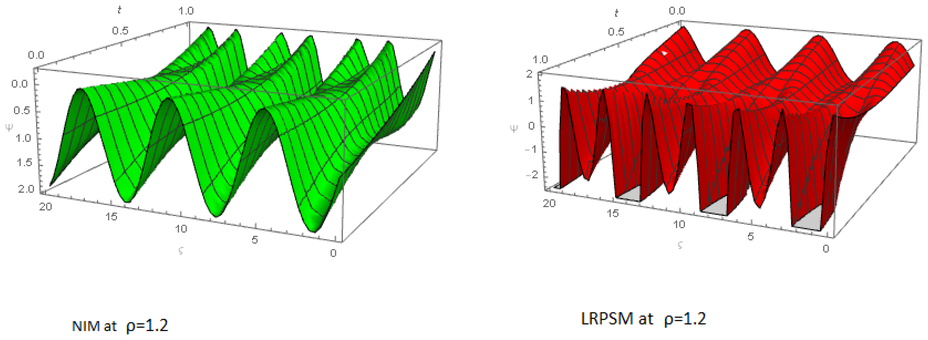
Figure 2.
Two-dimensional comparison of NIM and LRPSM solution for at different values of , , and , and .
Figure 2.
Two-dimensional comparison of NIM and LRPSM solution for at different values of , , and , and .
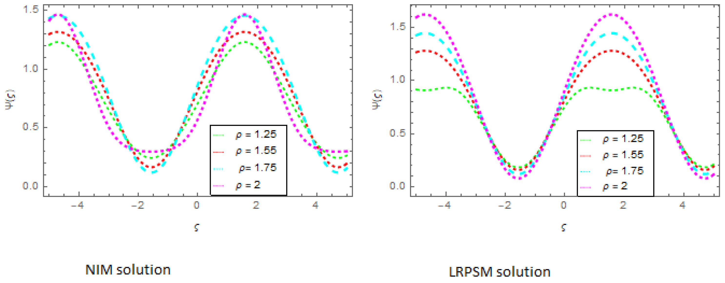
Figure 3.
Comparison of NIM and LRPSM solution graphs.

Figure 4.
Three-dimensional LRPSM and NIM solution for at different values of .

Figure 5.
Three-dimensional NIM solution for at different values of .

Table 1.
For example, we compare the solutions obtained using the proposed technique and the exact method for various fractional orders with .
Table 1.
For example, we compare the solutions obtained using the proposed technique and the exact method for various fractional orders with .
| NIM | LRPSM | NIM Absolute Error | LRPSM Absolute Error | |
|---|---|---|---|---|
| −1 | 0.161830 | 0.161830 | −1.45015 | −4.84885 |
| −0.9 | 0.219649 | 0.219649 | −9.26956 | −4.20187 |
| −0.8 | 0.285219 | 0.285219 | −1.81174 | −3.5230 8× |
| −0.7 | 0.357872 | 0.357872 | −2.77101 | −2.83933 |
| −0.6 | 0.436869 | 0.436869 | −3.76338 | −0.21777 |
| −0.5 | 0.521411 | 0.521411 | −0.47337 | −1.56448 |
| −0.4 | 0.610642 | 0.610642 | −5.61359 | −1.02418 |
| 0.3 | 0.703661 | 0.703661 | −6.32343 | −5.78561 |
| −0.2 | 0.799530 | 0.799530 | −0.67759 | −2.45844 |
| −0.1 | 0.897287 | 0.897287 | −6.88098 | −3.99668 |
| 0 | 0.995950 | 0.995950 | −6.55214 | 2.99566 |
| 0.1 | 1.094530 | 1.094530 | −5.71342 | −3.99701 |
| 0.2 | 1.192050 | 1.192050 | −4.30678 | −2.48219 |
| 0.3 | 1.287540 | 1.287540 | −2.29905 | −5.87823 |
| 0.4 | 1.380040 | 1.380040 | 3.11952 | −1.04656 |
| 0.5 | 1.468640 | 1.468640 | 3.49319 | −1.60733 |
| 0.6 | 1.552470 | 1.552470 | 7.17426 | −2.24876 |
| 0.7 | 1.630690 | 1.630690 | 0.112480 | −2.94595 |
| 0.8 | 1.702550 | 1.702550 | 0.155738 | −0.36714 |
| 0.9 | 1.767320 | 1.767320 | 0.199841 | −4.39613 |
| 1 | 1.824380 | 1.824380 | 0.242930 | −5.09083 |
Table 2.
For example, we compare the solutions obtained using the proposed technique and the exact method for various fractional orders of with .
Table 2.
For example, we compare the solutions obtained using the proposed technique and the exact method for various fractional orders of with .
| NIM | LRPSM | NIM Absolute Error | LRPSM Absolute Error | |
|---|---|---|---|---|
| −1 | 0.161830 | 0.161830 | −2.450 | −5.848 |
| −0.9 | 0.428538 | 0.428538 | −8.269 | −5.201 |
| −0.8 | 0.384187 | 0.384187 | −2.811 | −4.523 |
| −0.7 | 0.246887 | 0.246887 | −3.771 | −3.839 |
| −0.6 | 0.535480 | 0.535480 | −4.763 | −1.217 |
| −0.5 | 0.432147 | 0.432147 | −1.473 | −2.564 |
| −0.4 | 0.511532 | 0.511532 | −6.613 | −2.024 |
| 0.3 | 0.612678 | 0.612678 | −7.323 | −4.785 |
| −0.2 | 0.688420 | 0.688420 | −1.677 | −3.458 |
| −0.1 | 0.786217 | 0.786217 | −7.880 | −4.996 |
| 0 | 0.885960 | 0.885960 | −7.552 | 3.995 |
| 0.1 | 1.189150 | 1.189150 | −4.713 | −4.997 |
| 0.2 | 1.289131 | 1.289131 | −3.306 | −3.482 |
| 0.3 | 1.376450 | 1.376450 | −3.299 | −4.878 |
| 0.4 | 1.470030 | 1.470030 | 4.119 | −2.046 |
| 0.5 | 1.358941 | 1.358941 | 4.493 | −2.607 |
| 0.6 | 1.664810 | 1.664810 | 8.174 | −3.248 |
| 0.7 | 1.781581 | 1.781581 | 1.1124 | −3.945 |
| 0.8 | 1.812441 | 1.812441 | 1.1557 | −1.367 |
| 0.9 | 1.805231 | 1.805231 | 1.1998 | −5.396 |
| 1 | 1.786200 | 1.786200 | 1.2328 | −6.090 |
Disclaimer/Publisher’s Note: The statements, opinions and data contained in all publications are solely those of the individual author(s) and contributor(s) and not of MDPI and/or the editor(s). MDPI and/or the editor(s) disclaim responsibility for any injury to people or property resulting from any ideas, methods, instructions or products referred to in the content. |
© 2023 by the authors. Licensee MDPI, Basel, Switzerland. This article is an open access article distributed under the terms and conditions of the Creative Commons Attribution (CC BY) license (https://creativecommons.org/licenses/by/4.0/).
Share and Cite
MDPI and ACS Style
Noor, S.; Alshehry, A.S.; Aljahdaly, N.H.; Dutt, H.M.; Khan, I.; Shah, R. Investigating the Impact of Fractional Non-Linearity in the Klein–Fock–Gordon Equation on Quantum Dynamics. Symmetry 2023, 15, 881. https://doi.org/10.3390/sym15040881
AMA Style
Noor S, Alshehry AS, Aljahdaly NH, Dutt HM, Khan I, Shah R. Investigating the Impact of Fractional Non-Linearity in the Klein–Fock–Gordon Equation on Quantum Dynamics. Symmetry. 2023; 15(4):881. https://doi.org/10.3390/sym15040881
Chicago/Turabian StyleNoor, Saima, Azzh Saad Alshehry, Noufe H. Aljahdaly, Hina M. Dutt, Imran Khan, and Rasool Shah. 2023. "Investigating the Impact of Fractional Non-Linearity in the Klein–Fock–Gordon Equation on Quantum Dynamics" Symmetry 15, no. 4: 881. https://doi.org/10.3390/sym15040881
Note that from the first issue of 2016, this journal uses article numbers instead of page numbers. See further details here.