
Review of Chaotic Intermittency

1
Departamento de Aeronáutica, Instituto de Estudios Avanzados en Ingeniería y Tecnología (IDIT), FCEFyN, Universidad Nacional de Córdoba and CONICET, Córdoba 5000, Argentina
2
Departamento de Física Aplicada, ETSI de Aeronáutica y Espacio, Universidad Politécnica de Madrid, 28040 Madrid, Spain
*
Author to whom correspondence should be addressed.
†
These authors contributed equally to this work.
Symmetry 2023, 15(6), 1195; https://doi.org/10.3390/sym15061195
Submission received: 13 April 2023
/
Revised: 30 May 2023
/
Accepted: 31 May 2023
/
Published: 2 June 2023
(This article belongs to the Special Issue Symmetry in Nonlinear Dynamics and Chaos II)
Abstract
:Chaotic intermittency is characterized by a signal that alternates aleatory between long regular (pseudo-laminar) phases and irregular bursts (pseudo-turbulent or chaotic phases). This phenomenon has been found in physics, chemistry, engineering, medicine, neuroscience, economy, etc. As a control parameter increases, the number of chaotic phases also increases. Therefore, intermittency presents a continuous route from regular behavior to chaotic motion. In this paper, a review of different types of intermittency is carried out. In addition, the description of two recent formulations to evaluate the reinjection processes is developed. The new theoretical formulations have allowed us to explain several tests previously called pathological. The theoretical background also includes the noise effects in the reinjection mechanism.
1. Introduction
Chaos theory has many fields of investigation, such as the different routes to chaos. One route is chaotic intermittency, which has been observed in several subjects. Batchelor and Townsend, in the middle of the previous century, used the word intermittency to give an account of the fluctuating velocity in turbulent flows [1]. Subsequently, intermittency has been found in many and varied physical phenomena such as the nonlinear behavior of transient periodic plasma and conducting fluids [2,3,4,5], fluid mechanics and turbulent flows [6,7,8,9,10], Rayleigh–Benard convection [11], electronic digital oscillator [12], logistic map [13], Alfven wave-fronts and derivative nonlinear Schrodinger equation [14,15], premixed combustion [16], Lorenz system [17], coupled oscillators [18,19,20,21], catalytic reactors [22], Ginzburg Landau equation [23], solar cycles [24], spatiotemporal chaos [25,26], thermoacoustic instability [27], control chaos [28], etc. Furthermore, chaotic intermittency is also observed in systems in economics [29,30], medicine, [31,32], neuroscience [33,34], genetics [35], and marine biology [36,37]. Therefore, a more suitable understanding of chaotic intermittency can collaborate to describe these phenomena accurately. In addition, the correct description of chaotic intermittency possesses significance for systems whose precise equations are partially or totally unknown.
There are three classical routes by which continuous or discrete dynamical systems can evolve from regular functioning to chaotic behaviors: quasi-periodic route, period-doubling scenario, and intermittency [38]. In chaotic intermittency, the dynamical system solutions display alternation between regular or pseudo-laminar phases and chaotic bursts or non-regular phases. The laminar phases correspond to pseudo-equilibrium, pseudo-periodic solutions, and quasi-invariant objects close to them that the system may consume for a long time. On the other hand, the burst ones are consistent with chaotic evolution [39].
Approximately 50 years ago, chaotic intermittency was categorized into three different types, known as I, II, and III [17,40,41]. This classification was according to the fixed point eigenvalues in the local Poincaré map or the Floquet multipliers of the continuous-system periodic solution [38,39,42]. Later works introduced other types of chaotic intermittency such as on–off, eyelet, ring, and in–out, type-X, and type-V [43,44,45,46,47,48].
The monodromy operator multipliers determine the type of intermittency [49]. Type-I intermittency happens if the periodic solution loses its stability by a cyclic-fold bifurcation [50], then a multiplier goes away from the unit circle by the real axis across +1. Type-II intermittency is born in a sub-critical Hopf bifurcation or a Neimark–Sacker bifurcation [38,51]. Accordingly, two complex-conjugate Floquet multipliers gets out the unit circle. Therefore, it is a consequence of a bifurcation scenario for torus breakdown. A sub-critical period-doubling bifurcation generates a type-III intermittency. In this bifurcation, an unstable period-2 orbit encounters and destabilizes a stable period-1 orbit. Type-III intermittency presents a progressive increase throughout the laminar phase of a period-2 component in the motion [52]. In addition, a one-dimensional map showing a sub-critical period-doubling bifurcation possesses a positive Schwartzian derivative, :
Chaotic intermittency may be investigated using one-dimensional maps (Poincaré maps) [38,39,42]. These maps have two main characteristics: a particular local map and a reinjection process or reinjection mechanism. The specific local map depicts the type of intermittency. The reinjection mechanism returns the trajectories from the chaotic regime to the laminar one. Therefore, the reinjection mechanism determines the reinjection probability density function (RPD). It considers only points in the laminar region, but in the preceding period they have not been there. Note that the RPD is used to describe the reinjection process and is defined by the chaotic dynamics of the system itself. The probability of the reinjection points being in a particular sub-interval inside the laminar interval equals the integral of the RPD in the sub-interval. The RPD function specifies the probability that trajectories are returned (reinjected) into the laminar zone around to the unstable or even the vanished fixed point, and together with the local map outline all the dynamical features of the system.
The precise determination of the RPD function is extremely significant in correctly describing the chaotic intermittency phenomenon. In addition, the evaluation of the RPD function from experimental or numerical is a hard task due to the large amount of data involved, and it is difficult to estimate the statistical fluctuations generated in the numerical result and experimental data. Several strategies were utilized to calculate the RPD function. Most results in the classical theory of chaotic intermittency were obtained considering uniform reinjection inside the laminar interval [41,42,53]. Other implemented RPD functions were constructed using specific characteristics of the nonlinear processes. For example, in type-I intermittency the reinjection was restricted to the fixed point [54], and for the intermittency of type-III the RPD function was assumed proportional to , with constant [55]. Notwithstanding, these RPD functions cannot be generalized to other nonlinear systems.
Two new methodologies together with their theoretical background to obtain the RPD function were introduced in recent years. One of them is the M function methodology [56,57,58,59,60,61,62,63,64]. This methodology introduces a generalized power law for the RPD. It has been shown to be very accurate for a broad class of one-dimensional maps showing type-I, II, III, and V intermittencies. In addition, the M function methodology includes the classical approximation because it contains the uniform reinjection as a particular case. The second one is called the continuity technique. It utilizes the Perron–Frobenius operator to compute the reinjection probability density function. In the same way as the methodology of the M function, the continuity technique has been shown to be accurate for several maps displaying different types of intermittency [65,66,67].
To more precisely describe the intermittency phenomenon, other statistical functions are used, such as the probability density of the laminar lengths (), the average laminar length (), and the characteristic relation (). Nonetheless, these functions depend on the RPD. To calculate them, we previously have to know the reinjection probability density function [39,42].
The RPD and the other statistical functions used to describe the chaotic intermittency are affected by the noise and the lower boundary of reinjection (LBR). The M function methodology has been extended to incorporate both phenomena [68,69,70].
This paper presents a review of chaotic intermittency, with an emphasis on the evaluation of the RPD and other statistical functions.
2. Types of Chaotic Intermittency
Let us analyze a periodic solution of an autonomous continuous-time system. It is stable for some values of the control parameters. At that time, if a control parameter is modified until the periodic solution loses stability, the development of the solution shall depend on how the Floquet multipliers go away from the unit circle in the complex plane [38,42,53]. Note that the metamorphoses of a family of solutions around a closed orbit is a complex problem of bifurcation theory [71].
The existence of type-I, II, and III intermittency depends on the monodromy operator multiplier. Type-I intermittency occurs by a cyclic-fold bifurcation, then a multiplier goes away from the unit circle across +1. Type-II intermittency is born in a sub-critical Hopf bifurcation (or a Neimark–Sacker bifurcation), in which two complex-conjugate multipliers move away from the unit circle. Finally, type-III intermittency appears if a multiplier gets out the unit circle by −1, and a sub-critical period-doubling bifurcation happens [38,49,51].
2.1. Type-I Intermittency
Type-I intermittency is probably the most studied intermittency. Numerous books and papers describe it. When a control parameter surpasses the threshold value, type-I intermittency is born in a cyclic-fold bifurcation, then the fixed point of the Poincaré map vanishes.
To introduce the classic theoretical model for different types of intermittency, we use the following nonlinear system:
where is the variable vector, is the vector field, and is a control parameter.
For , a monodromy operator multiplier (or Floquet multiplier) related with a periodic solution of Equation (2) goes away the unit circle by +1, starting a discontinuous or catastrophic cyclic-fold bifurcation (bifurcation of codimension-one). The manifold of this multiplier possesses significant information related to intermittency—in other directions, there is dissipation [38]. Accordingly, to understand intermittency, we can study only a one-dimensional map associated with this manifold , where .
For type-I intermittency, the characteristic local map is [72]:
The value of control parameter determines the number and stability of the fixed points of this map. For , two fixed points exist. One is stable, and the other is unstable. When , both fixed points collide and meet in only one fixed point. Finally, for , the map does not have fixed points (tangent bifurcation).
When , there is a narrow channel. The distance across the channel depends on . The trajectories spend a long time crossing the tunnel. The zone around the vanished fixed point determines the laminar interval. Accordingly, inside the laminar interval the trajectories are near to the disappeared fixed point. Nevertheless, they can not come to it.
To achieve type-I intermittency, in addition to the local map, a reinjection mechanism has to exist. The local map is given by Equation (3); however, the reinjection depends on the nonlinear map. Outside the channel, the trajectories show chaotic behavior. However, they return inside the narrow channel by the reinjection process. Usually, each trajectory returns to different points inside the laminar interval. The reinjection probability density function, , determines the probability that trajectories are reinjected in the x-point. Therefore, it is the core of the statistical performance of chaotic intermittency.
In this subsection, we consider that the lower boundary reinjection point (LBR) coincides with the lower limit point of the laminar region. Consequently, the reinjection process occurs in the complete laminar interval [39].
We have previously established the significance of the RPD function in describing the chaotic intermittency phenomenon. The classical formulation for chaotic intermittency establishes a constant RPD. Consequently, reinjection probability is the same for all points in the laminar interval:
where k is a constant value. Equation (4) implies uniform reinjection.
The laminar length or the length of the laminar interval is the number of iterations needed by the trajectory to cross the laminar interval. Accordingly, it is an integer number. We can describe the laminar length as the “time” utilized by each trajectory to move through the laminar zone. Note that reinjection point x determines the length of the laminar interval. For type-I intermittency, a reinjected trajectory progresses through the narrow channel until it moves away from the laminar interval. For , we can approximate the map (3) as a differential equation [42]:
where we have considered . Integrating this equation, we obtain the laminar length, l:
where c is the upper limit of the laminar interval. Note that the laminar length does not depend on the reinjection mechanism; it only depends on the local map given by Equation (3).
The probability density of the laminar lengths, here called , outlines the probability of finding laminar lengths between l and [42]:
in this last equation, is the inverse of the laminar length given by Equation (6):
The average laminar length, here called , is calculated as
where is the highest laminar length, which is obtained as . Note that .
The characteristic relation describes the dependence of average laminar length, , with the control parameter, . For type-I intermittency, if , it results in:
2.2. Type-III Intermittency
Type-III intermittency starts in a sub-critical period-doubling bifurcation. Therefore, an unstable period-2 orbit collides with a stable period-1 orbit and destabilizes it. A Floquet multiplier moves away to the unit circle by , while the others multiplies are inside the unit circle. The information to describe type-III intermittency is in the manifold related to the unstable Floquet multiplier. Type-III intermittency can be analyzed using a map associated with this manifold, [38,39].
A local map can be written as
where [52,58], and and depend on the dynamic process [38]. is a fixed point for all . It is stable for and unstable for .
Note that the type-III intermittency behavior is different to that of type-I. The fixed point does not vanish; it only loses its stability. Furthermore, there is not a channel between the map and the bisector.
To examine type-III intermittency, the second iteration of Equation (12) is built:
For small values of and , the second iteration of map (13) reduces to [39]:
where .
For , the map (14) has two behaviors depending on the sign of the cubic term coefficient, a:
- . There are three fixed points: and . When loses its stability, the other two fixed points are stable and attract the trajectories. There is a supercritical pitchfork bifurcation, and intermittency does not occur.
- . For , is the only real fixed point, which is unstable. If there is a reinjection mechanism, type-III intermittency occurs. It is related to a sub-critical pitchfork bifurcation of , or associated with a sub-critical period-doubling bifurcation of . Note that implies . For this reason, several studies utilize Equation (14) as a local map instead of Equations (12) or (13).
If exhibits a subcritical period-doubling bifurcation, the Schwartzian derivatives have to be positive:
For , this equation implies . Accordingly, for one-dimensional maps, type-III intermittency occurs if .
For the classic formulation of chaotic intermittency, the RPD is constant, and it has to satisfy the normalization condition:
then .
Following the procedure used for type-I intermittency, the laminar length for a reinjected point x is:
where is the laminar length for the map. For simpleness we have used . Consequently, the laminar length for the map, given by Equation (12), results, .
The probability of laminar lengths, , results (see Equation (7)).
The average laminar length is [39]:
The last equation verifies when . Note that the characteristic relations for type-I and type-III intermittencies have the same form. The length of the laminar phases rises when decreases.
2.3. Type-II Intermittency
Type-II intermittency happens in two or higher-dimensional maps. It occurs when two complex-conjugate eigenvalues of the fixed point go away from the unit circle, and a sub-critical Hopf bifurcation appears. A two-dimensional manifold is related to the two eigenvalues, which is spanned by the eigenvectors of the complex conjugate eigenvalues. We can study the dynamics of this manifold because the absolute values of other eigenvalues are less than 1. The complex monodromic eigenvalues can be expressed as , where is an angle. The local dynamic can be described by a two-dimensional map [38]
where is the control parameter. a, b, and q are constants. For , type-II intermittency can occur.
To explain type-II intermittency, the same statistical variables studied for type-I and type-III intermittencies are calculated. The classical formulation implements a constant RPD. Nevertheless, the other statistical variables are not constant. For , Equation (20) can be approximated as:
Hence, we have:
where c is the upper limit of the laminar interval and x is the reinjection point. Note the laminar interval is .
The probability density of the laminar lengths, , can be obtained from Equation (7):
The average laminar length is
where the RPD is constant, , where we have utilized the normalization condition given by Equation (16).
The characteristic relation is obtained from Equation (24) for ; it results . Note that the characteristic relation for type-II intermittency is similar to those calculated for type-I and type-III.
2.4. Type-V Intermittency
Type-V intermittency occurs if a stable fixed point in a non-differentiable, even discontinuous, map meets with a non-differentiable or discontinuous point. Refs. [73,74,75] introduced this idea approximately 30 years ago.
Types-I, II, and III intermittencies occur on differentiable maps. Nevertheless, a different process can happen if the map has discontinuous or non-differentiable points. If a control parameter changes so that one non-differentiable point (NPD) moves in the direction of and meets with a stable fixed point, then a channel between the bisector and the map occurs.
Type-I intermittency occurs at a tangent bifurcation where the map is tangent to the bisector line at critical, and the eigenvalue associated with the critical point is +1. Notwithstanding, for a non-differentiable point, the map at this point is non-differentiable or discontinuous, so that there is no tangent. Then, a tangent bifurcation does not exist for a non-differentiable point. For some maps, there are two slopes around the non-differentiable point, one for the left part of the map and the other for the right one.
Let us to analyze the following map displaying type-V intermittency [73]:
where is a random number in the interval and is the discontinuous point. A and B are settled on to satisfy that the reinjection happens below the intersection between the bisector line with the function . The parameters a and b govern the modification of the function with the control parameter . For decreasing , moves toward the diagonal. For , is a fixed point: . At the discontinuity point, the slope of is , which is assumed independent of . The parameters a and b can be written as function of s and :
If we consider that , , and random reinjection, the average laminar length results:
where is independent of . For :
and for :
The scaling laws for other two maps were evaluated in [74]. The the right part of the first map is:
where a satisfies: , and the control parameter is . For , there is a critical point.
The laminar length is:
If a random reinjection mechanism with probability is considered. The average laminar length results:
where x and are the entrance and the exit points, respectively.
2.5. Type-X Intermittency
Type-X intermittency was introduced in [44], and it is related to type-I intermittency. Notwithstanding that both intermittencies are different, each one possesses particular properties.
For type-I and type-X intermittencies, the local is:
where is an unstable fixed point, and is the control parameter.
Type-X intermittency displays a hysteresis mechanism together with a regular reinjection process where the trajectories are returned at the same point. This behavior, close to the threshold where the chaotic phase vanishes, is different to type-I intermittency. For type-X, there is no channel. Consequently, the laminar length is determined by the distance between the reinjection point and the unstable fixed point, and by the gradient of the map near this zone [39].
To investigate the local behavior of trajectories close to the unstable fixed point, the local map around the fixed point can be approximated by a straight line. In that case, the bisector line and the local map determine an X-shape. Accordingly, it is possible to use this assumption to evaluate the average laminar length and its dependence on the control parameter . Remember that all trajectories are reinjected at the same point after each chaotic interval; is the distance separating the reinjected point from the unstable fixed point. For small , it depends linearly on [44]:
The linearized map around the unstable fixed point can be written as:
for , we can approximate it as:
If the iterates advance from the reinjection point—defined by —to the laminar interval upper limit c, the laminar length results:
2.6. On–Off Intermittency
On–off intermittency presents sudden changes between approximately constant periods or static states and bursts of large-intensity irregular oscillations. The “off” states correspond to nearly constant periods. The “on” states show oscillations of large-intensity. These burst periods depart and return suddenly to the “off” states [45,76].
For the previously analyzed intermittency types, a trajectory of the map spends large periods of time near an unstable or vanished fixed point. This fixed point of the Poincaré map is consistent with a periodic orbit for the continuous system. However, the system states can spend a long time close to other unstable quasi-invariant or invariant objects. Accordingly, intermittency can happen nearby the quasi-invariant or even invariant objects where fixed points are solely singular cases. On–off intermittency has been observed in coupled chaotic oscillators [77]. Moreover, in Ref. [78], coupled oscillators exhibiting the coexistence of chaotic attractors having on–off and Type-I intermittencies among other chaotic scenarios has been reported.
We consider a state space of dimension . In this space, there is an unstable object inside the hyper-surface, , with . Near this object, on–off intermittency can happen. In addition, the co-dimension can be large, and on–off intermittency could occur for both deterministic and random development in the complementary state space [45].
The simpler version of on–off intermittency necessitates two components: an invariant object and orbits going inside and departing every small neighborhood of the invariant object. A dynamical system possessing these elements can be written in the following form:
where and . Note in Equation (41) the derivative of is independent of ; nevertheless, the evolution depends on . Subsequently, the dynamical system display a skew product structure.
Additionally, the hyper-plane is an invariant object, which is unstable when the control parameter goes beyond a critical value : . If the trajectory evolves in such a way that visits two zones, such as moving above and below the critical control parameter , and if the spent time by the trajectory in both regions is proper, then on–off intermittency can occur. Note that when and , the classical intermittency mechanism can be recovered.
The process supporting on–off intermittency is the reiterated change of a dynamical variable across a bifurcation point of another dynamical variable. The first variable adjusts a time-dependent control parameter, which affects the second variable adopting the intermittent signal.
The possibility to control on–off intermittent dynamics, that is to stabilize a trajectory in a desirable state, has been investigated previously (see [77] and references therein). The control of the on–off intermittent dynamics by using a closed-loop algorithm requires full knowledge of the system. However, to avoid this issue, an open-loop control of a chaotic dynamical system that exhibits on–off intermittency has also been proposed [79].
2.7. Eyelet Intermittency
The eyelet intermittency occurs close to the phase synchronization boundary of chaotic coupled systems. It can be described by the phase synchronization of unstable periodic saddle orbits embedded in chaotic attractors [80].
Additionally, eyelet intermittency can arise nearby the phase synchronization boundary of a periodically forced chaotic system. This was introduced through the investigation of the phase synchronization onset, which corresponds with a collision between an attractor and a repeller.
Let us study the following two-dimensional map:
Physically, the map is the stroboscopic characterization of a continuous-time chaotic oscillator externally excited by a periodic force. The system given by Equation (42) is composed of the perturbed tent map coupled with the circle map.
The variables x and are the amplitude and phase of the oscillator, respectively. The parameter is related to the force amplitude. For autonomous systems, it verifies . The detuning between the periods of oscillations and external force is described by the terms and . In addition, is proportional to the external force frequency. The chaotic modulation of the phase motion is described by .
The analysis of the characteristics of unstable periodic orbits embedded in chaotic attractors is an approximation to studying the phase synchronization of chaotic oscillators [81,82,83]. For the system (42), a phase-locked zone with zero rotation or winding number arises for each trajectory (Arnold’s tongues).
In the phase-locked region, there are two orbits for phase for each orbit of the tent map. These two orbits are unstable in the x direction. However, in the direction, one is stable and the other is unstable. At the synchronization boundary, a saddle-node bifurcation happens. These orbits disappear, and a state with a nonzero rotation number arises.
A zone where all the phase-locked regions overlap is named the region of full-phase synchronization. It is limited by the phase-locked regions of the periodic orbits possessing the minimal and maximal average period.
Near the boundary of the full-phase synchronization region, the repeller and attractor approach each other. At the transition point, a saddle-node bifurcation of one of the unstable periodic orbits happens, and a attractor–repeller collision occurs. A few cycles miss the phase locking, permitting the phase to slip (most cycles continue phase-locked).
The dynamic in the direction, which is a weakly unstable direction, is driven by the saddle-node bifurcation. Consequently, the characteristic time of phase slip is:
where is at the bifurcation point.
For a phase slip to appear, a chaotic trajectory has to stay at least a time near the vicinity of the direction (weakly unstable direction). However, the x direction is strongly unstable, and the distance to the weakly unstable direction is:
where is the multiplier in the strongly unstable direction.
For at least one phase slip to emerge, the initial distance should be small:
where collision C is a constant. This region is called the eyelet and is exponentially small.
Nearby the border of the phase synchronization region, the phase difference possesses time intervals of phase synchronized behavior, which are intermittently interrupted by abrupt phase slips.
Near the boundary of the phase synchronization, two intermittency types may emerge when the natural frequency of the system and the external signal frequency are moderately detuned: type-I and eyelet intermittencies. Then, two critical values exist [84].
There are two coupling strengths, and (), for two coupled chaotic systems. These strength values are the boundaries of different dynamical behaviors. Type-I intermittency appears for values of less than , i.e., . For values satisfying , there is eyelet intermittency, and for the phase synchronization region happens [84].
The equation relating to the mean length of the laminar phases, , with the control parameter is:
where is constant.
The eyelet intermittency has been found in nonlinear systems by numerical calculations and experimental investigations [85].
A more recent investigation observed that noisy type-I and eyelet intermittencies can display the same type of dynamic. Nevertheless, these intermittencies can be found under different conditions [84].
For a deeper analysis of eyelet intermittency and synchronization, the readers can utilize the following references [47,81,83,84,85].
Another type of intermittency, called ring, also occurs near the boundary of the phase synchronization zone. Nevertheless, it happens for high initial frequency mismatches of two coupled systems [48].
2.8. Spatiotemporal Intermittency
A brief description of spatiotemporal intermittency is carried out. Spatially extended systems—systems with spatial extension—may generate intermittency. Nonlinear partial differential equations (PDEs) represent these types of systems. In consequence, it is a very vast research subject.
The dynamics of the viscous fluid flow is described by the Navier–Stokes equations [86,87,88,89]. These equations are an example of a spatially extended system:
where is the velocity vector, p is the pressure, is the density, is the viscosity, and t is the time.
For incompressible flow, we coupled the Navier–Stokes equations with the incompressible continuity equation:
On the other hand, for compressible flow the continuity equation results:
If the evolution of the variables of a system such as Equation (47) coupled with Equations (48) or (49) are random in time, it is possible to speak about spatio-temporal chaos. Additionally, spatio-temporal chaos could be considered a kind of temporally chaotic pattern-forming mechanism. In addition, if these variables show a spatially irregular behavior, the process can be called fully developed spatio-temporal chaos.
Spatiotemporal intermittency is an indication of spatiotemporal chaos and full spatiotemporal chaos. It has been observed in several experimental works [90,91]. In addition, spatiotemporal intermittency can occur in spatially extended dynamical systems. Each space-time point of these systems can show pseudo-laminar and pseudo-turbulent states. For pseudo-laminar states, the spatial behavior is regular. Despite this, the temporal dynamics could be both chaotic and regular. On the other hand, pseudo-turbulent states exhibit no recognizable regularity either in space or in time [92].
Spatiotemporal intermittency alternates in both time and space pseudo-laminar and pseudo-turbulent states. In addition, this type of intermittency can be understood as a transition state between regular and chaotic behaviors, where the domains of each phases possess well-defined contours.
Long-time averages of spatial variables are implemented to calculate the distribution amplitudes of pseudo-laminar and pseudo-turbulent states. Both distributions exhibit an exponential decay, which is connected with the average extension of the pseudo-laminar and pseudo-turbulent phases [93].
Furthermore, long transient behaviors for spatially extended systems can be described by spatiotemporal intermittency [94,95]. Additionally, some of these states have suitable long lifetimes to evaluate steady statistical variables. Consequently, spatiotemporal chaos can exhibit this type of intermittency. Then, spatiotemporal intermittency could contribute to a spatiotemporal chaotic attractor [92].
2.9. Crisis-Induced Intermittency
In dynamical systems, Ref. [99] introduced the world crises. A crisis takes place through a collision between an unstable periodic solution with a chaotic attractor. During a crisis, as a control parameter is varied, the chaotic behavior of dissipative dynamical systems experiences sudden qualitative modifications.
According to Ref. [100], there are three different types of crisis: exterior or boundary, interior, and attractor merging. The three types of crisis depend on how the chaotic attractor is abruptly modified (discontinuity of the chaotic attractor).
The chaotic attractor is suddenly destroyed by a boundary crisis. It occurs when a control parameter moves across a critical value . The boundary crisis is also called an exterior crisis [38]. For an interior crisis, the size of the attractor suddenly expands when the control parameter passes through the critical value . Finally, for an attractor merging crisis, if the control parameter goes through the critical value, two or more chaotic attractors of the system merge in only one chaotic attractor. The new attractor can acquire a larger size than the union of the previous chaotic attractors for . The last two crises, interior and merging, are called explosive bifurcations [38].
It is a quadratic map (one-dimensional). This map, for , possesses two fixed points:
For , a tangent bifurcation appears, which generates stable and unstable fixed points, and . The stable fixed point misses stability at by a period-doubling bifurcation. For larger values of a, a cascade of period-doubling bifurcations occurs with an accumulation point at . For , there is a chaotic attractor that shows many tiny windows of periodic solutions. At , the chaotic attractor merges with the unstable fixed point, and it vanishes by an exterior crisis or blue sky catastrophe [38].
For , there is an interior crisis. At , the chaotic attractor vanishes, and three tangent bifurcations appear. For each one of these bifurcations, stable and unstable fixed points start. At , the stable period-three orbit sustains a period-doubling bifurcations sequence. At , the three chaotic bands and the unstable period-three orbit merge (an interior crisis occurs). Therefore, the chaotic attractor modifies from three chaotic bands to a one-band chaotic attractor [39].
For a slightly larger than , the chaotic attractor trajectory spends long time intervals around the attractor before the interior crisis (pseudo-laminar region). These intervals are interrupted by bursts, where the trajectory departs to an extended region (chaotic region). Following that, the trajectory comes back to the zone around the chaotic attractor before the interior crisis, and this process continues. This behavior is called crisis-induced intermittency [99].
2.10. Fine Structure in Intermittency
Refs. [101,102] describe a fine structure in intermittency. These papers study numerically type-I intermittency. The Lyapunov exponent, the average laminar length, and the mean value of the dynamical variable, x, for several values of the control parameter , are calculated. The map analyzed in [101] is:
where z takes the values 2 and 4. For this map, the characteristic relation is [101]:
The Lyapunov exponent is calculated as:
where . The mean value (average) of the dynamical variable is:
where the total number of iterations was .
The three statistical variables, , , and , show oscillations. The oscillation amplitudes are larger for the Lyapunov exponent and the mean value of the dynamical variable.
If we do not consider the oscillations, the results display the traditionally known characteristic relation (see Equation (10)). The relation of the with can be written as:
The relation of the Lyapunov exponent with the control parameter results:
When the control parameter verifies , the oscillations scale as for , and for .
It is a piecewise linear map. This map, for , possesses a fixed point , which vanishes for .
The authors, using numerical simulations, found that the Lyapunov exponent, average laminar length, and the statistical moment of the chaotic variable display logarithmic periodic oscillations. Accordingly, the fine structure produced by the oscillations generates a signature of nonlinearity, which could be utilized to reach supplementary information about the characteristic exponents.
2.11. Two-Dimensional Intermittency
Some concepts to describe two-dimensional type-I intermittency are introduced in Ref. [103]. It occurs around a tangent bifurcation point similar to the one-dimensional type-I intermittency.
The first-order difference equations system, in m-dimensional space, can be written as:
where the vector , with being the m-dimensional Euclidean vector space. For , high-dimensional intermittency can appear. For two-dimensional vector space, , the Equation (60) is reduced to:
In one-dimensional type-I intermittency, there is a channel where the trajectories spend a long time moving across it. The channel amplitude—the distance between the diagonal and the map—is determined by the control parameter .
To study high-dimensional intermittency, an m-dimensional diagonal hypersurface (DHS) has to be defined [103]. For two-dimensional vector space, ; the DHS is the surface specified by and . The map forms a channel between the DHS and the map. The pseudo-laminar behavior happens as long as the trajectory crosses this channel.
The local map for type-I intermittency in one-dimensional vector space is given by a quadratic equation (see Equation (3)). In two-dimensional intermittency, this map can be written as:
where and are arbitrary coefficients. In an iterative process, given a point , the subsequent point can be calculated as the addition of two vectors. The first one is in the x-direction, and the second is in the y-direction. As a consequence, the channel is not identical for all trajectories. To deal with this phenomenon of high-dimensional intermittency, a new parameter, named channel distribution function (CDF), has to be considered [103].
In two-dimensional intermittency, three trajectory categories can appear: limit cycle, quasiperiodic, and chaotic. The CDF depends on the trajectory, and it is distinct for each trajectory type. A limit cycle displays one trajectory in the plane. Then, the channel is unique. Its functioning is similar to that of one-dimensional intermittency. The quasiperiodic one generates a variable channel with a uniform CDF. Lastly, chaotic trajectories produce channels with fractal structures. Therefore, the conduit is not unique for quasiperiodic and chaotic trajectories. Consequently, a multichannel behavior happens, which is described by a probability distribution, or CDF. For this reason, the average laminar length depends on the CDF.
In Ref. [103], the authors calculated the average laminar length for the three trajectory types. For a limit cycle, the CDF verifies, , where delta is if and if . The characteristic relation, connecting the average laminar length with the control parameter, results:
For a quasiperiodic trajectory, the CDF is uniform, , where constant. In this case, the scaling law is:
where is the nearest channel width.
For a chaotic trajectory, the channel exhibits a discrete fractal structure. Consequently, can be represented by a sum of delta functions. The higher delta function related to the nearest channel width governs the average laminar length, :
3. New Formulation of the Chaotic Intermittency
In Section 2, we have seen many approximations that have been used in the literature to describe the RPD function. A more extended approach is to consider RPD as uniform and thus independent of the reinjection point (see for instance [40,42,55,104,105,106,107,108,109]). For the uniform reinjection, the more important expressions as the probability density of the length of laminar phase, , was obtained, along with the characteristic exponent , as we have shown in Section 2. Beside uniform reinjenciton, other investigations consider a limit approximation where the reinjection is only in a fixed point [54,107]. Previously, evidence was found on systems with intermittency whose statistical properties do not fit with the classical expected result derived for a uniform reinjection. An experimental Poincaré map with a gap around the fixed point was also reported. Note that this fact shows a non-uniform reinjection [56,104,110].
This demands a generalization of the RPD in order to include, in a generalized theory, every particular case that was not well explained by the classical intermittency theory.
This section is devoted to explaining this mentioned generalization and to extend the classical results on intermittencies.
3.1. The Reinjection Probability Density Function (RPD)
Let us consider the map described in Section 2, where
is a general one-dimensional map having intermittency.
Firstly, let us generalize the local dynamics corresponding to the three types of intermittencies around the unstable fixed point, that is, for type-I intermittency, the local map determined by:
where represents the weight of the nonlinear component and is a small control parameter (). The laminar behavior of type-II and type-III intermittencies around the fixed point are given by the following maps:
For , the fixed point becomes unstable; consequently, the trajectories slowly escape from the fixed point, preserving orientation for type-II and reversing orientation for type-III intermittency. Note that the nonlinear component in Equation (67) is not necessary quadratic, and for type-II and type-III it can be in Equations (68) and (69). Note that this restriction corresponds only to classical local maps (see Equations (14) and (20)). In any case, for , for type-II and type-III there is an unstable fixed point at , but for type-I there is not a fixed point and the trajectories move slowly along the narrow channel formed with the bisecting line.
To fix ideas, let us consider an illustrating model having type-II intermittency:
where
and is the root of the equation (see Figure 1). Note that determines the laminar dynamics, whereas determines the reinjection mechanism from the chaotic region into the laminar one (see green arrow in Figure 1). The RPD, denoted by , drives the statistical distribution of the reinjected points and is determined by the shape of in the chaotic region, that is . On the other hand, in the laminar region the origin is always the fixed point of , and for it is stable; however, it is unstable for , and the mapped points of a starting point closed to the origin increases in a process determined by and p. A chaotic burst occurs when becomes larger than , which will be interrupted when goes again into the laminar region mapped by , which determines the RPD. In the earlier paper [40], uniform reinjection was observed in the case of the map (70)–(71) for and . In [57], the following generalization of the reinjection mechanism was proposed:
where for the map studied in [40] is recovered. Let us estimate the behavior of in a neighborhood of for the case of , but before embarking on a discussion concerning RPD for , it is interesting to note the relationship between the RPD and the probability measure of an interval given by:
where denotes the characteristic function of the interval defined as:
Hence the probability measure gives the frequency of the signal in a specific interval of the attractor, and it depends on the invariant density, , by the follow integral:
Note that in our scenario . Let L be the laminar region and s an subset in L, that is, . In order to evaluate the probability, , according to definition (73), we split the whole data series into three subsets:
having an empty intersection between them:
with the following definitions. Firstly, we consider , and in the preceding period it has already been there, that is and . Now let us consider the following case, , but in the preceding period it has not been there, hence and . For the last case, we have . Note that is given by:
where the last term in Equation (78) is not necessary because, by definition, it is zero. The first term is just the probability of finding a point in s when, in the preceding period, it had already been there. Let us consider that , then the second term in the RHS of Equation (78) is, by definition, the RPD, called here , and is determined by the following relation:
where the weight, w, is introduced to fit to one and normalize the function over the whole laminar interval, L. We note that the fundamental characteristics of intermittency depends on , as for example, and the characteristic exponent , which are usually used to characterize the intermittency type, as will be seen below. Regarding the reinjection mechanism (72), for it is interesting to analyzed the behavior of of in a neighbor of . Note that every point reinjected in the laminar region, that is in the interval , are coming from the points near to (see green arrow in Figure 1). Consequently for , all points in the interval are mapped into the interval , where . This means that the probability of finding a point in to be reinjected into the interval is equal, where we denote the derivative of the function by . Hence, we conclude that , where we introduce the weight k to normalize on the whole interval . Note that is normalized only on the laminar interval; hence, we have .
Finally, can be approximated as follows:
For expression (80), evaluated for the function given by Equation (72), we have:
where is the derivative of function . In the first approximation of in the interval , we can consider as a constant and the density as uniform, and we get the following reinjection probability density:
where b is a normalization constant given by Equation (159). Note that the function RPD strongly depends on parameter , which determines the curvature of the map in the colored region in Figure 1. Only the points in the colored region are mapped into the laminar region. In [57], a numerical verification of Equation (82) is presented. Moreover, the power law (82) was verified for many one-dimensional maps, including the so-called “pathological” cases that deviate significantly from the classical predictions [59,111]. Moreover, the power law (82) has been observed in the Poincaré map of an experimental 3-D system made by an electronic circuit [112].
Note that the classical uniform RPD holds for the map of Figure 1 only in the case of , where is not an extreme point.
To evaluate the effect of LBR , we consider the following map as having type-I intermittency (see Equation (70)):
where determines the nonlinear term of the reinjection mechanism, whereas is the root of the equation . The new parameter is the so-called lower boundary reinjection point (LBR), defined by the limit value for the reinjected points from the chaotic region, as shown in Figure 2. Note that the statistical behavior of the intermittency strongly depends on the value of the LBR [63,69,106,113]. In the case of Equation (83), where , the RPD includes the parameter as follows:
From Equation (84), it follows that if , the RPD increases without boundary for , as shown in Figure 1 for . On the contrary, for , the RPD decreases when . Note that for we have two possibilities for the RPD, that is, convex or concave, which are separated by (see Figure 1).
Note that in these cases we have . In fact, for , the integral (79) does not converge.
As a consequence of the power law (84), a hole can be observed in the local map around the fixed point . Behind this fact, two different phenomena can be identified. On one hand, if the endpoint of the holes should be , hence there are not reinjected points around . On the other hand, for a hole can be observed in the experimental or numerical realizations, even in the case of , because we have . Note that, in this case, the gap length is not determined by and it decreases as the number of points increases, and for a long enough time, the gap can disappear [56,57]. The two free parameters determining the RPD (84), and , can be obtained from data series and also from the analytical definition of the map. This point will be explained in the following sections.
3.1.1. RPD from Data Series
In this case, we use the following integral characteristic [57]:
where is a suitable “starting” point. The function was used for the first time in a electronics circuit with intermittency [56], and it has been broadly extended due to being a linear function for a RPD given by Equation (84); consequently, the function is a useful tool to evaluate the parameters and .
Note that is an integral characteristic, hence its numerical evaluation is more robust than the direct estimation of . This allows reducing statistical fluctuations produced by a relatively small data set or due to high levels of noise [57,58,59]. Because is an average over reinjection points in the interval , we can write:
where the data set (N reinjection points) has been previously ordered, i.e., . In the case of RPD given by Equation (84), the function should follow the linear law:
where and can be approximated by . Equation (87) determines the corresponding RPD:
Note that by a simple least squares fitting we can estimate the parameters of the straight line (89) that determine the RPD given by Equation (90).
Figure 3 shows different RPD depending on exponent for and . The corresponding function depending on according to Equation (90) is also shown.
For , we recover the classical approach of uniform RPD, that is, , whereas for RPD it goes to ∞ as . On the contrary, when , we have . Note that in this last case we have two possibilities for the RPD, concave or convex, split by the slope (see Figure 3).
The evaluation of the function allows a more reliable numerical and experimental access than the RPD, . We have numerically verified Equation (89) for a broad class of maps. We highlight that the slope, m, can be different from . However, we always obtain .
In numerical or experimental data series there is a huge amount of data, which can include randomness. The M function methodology evaluates a mean value, reducing the randomness and allowing extraction of the physical information stored in the data series.
3.1.2. RPD from the Analytical Definition of the Map
Following the results of [111], let us analytically estimate the RPD by means of parameter of Equation (82). Let us consider a direct reinjection from the extreme point, which is the blue line on the minimum of the map in Figure 1. In this case, the map around the extreme point can be approached by , where d is a suitable constant and the value of is given by the next indeterminate limit:
To convert the limit (91) to an evaluated one, we can apply the L’Hopital rule. Note that usually we will get an indeterminate limit again. In general, when we have for , where indicates the i-derivative of ; hence, by using the L’Hopital theorem times, we obtain the following limit:
Notice that if the derivative exists, the limit (92) gives , and in the following Equation (82) we have:
where , as corresponds with an RPD generated in a maximum or in a minimum.
Note that from Equation (93) two natural limits appear. For , the uniform reinjection is recovered, and on the other hand, for , the RPD collapses into a -function. It is interesting to note that because of being an extreme point, the values of q in Equation (93) are restricted to odd natural numbers.
Let us study an indirect reinjection given in maps such as (119), where to reinject into the laminar region points lying around the maximum, two or more iterations of the map are necessary.
A similar scenario can be observed for maps , defined by a composition of single ones . See, for instance [41,82,106]. Hence, for a general case we consider the composed map:
where the function has an extreme point at that can be be mapped into the laminar region. In this case, points near are mapped after successive application of the functions, according to the composed map (94). In Ref. [111] we have shown that, even in this case, the RPD can be approximated by applying Equation (92) only to the function , instead of using the complete function, Consequently, the estimation of in the case of a map defined like Equation (94) is given by:
By this method, it is possible to estimate parameter by evaluating the number of null derivatives that have only the map with extreme points. To show how this method works, let us apply it to three cases of pathological maps that produce an important deviation of the main result expected from the uniform distribution of the RPD [111]. These maps (see Figure 4) were considered in [113] and estimated the RPD by numerically solving the Shaw relation [114], but following our result it is very easy to use an analytical approach. The first map considered is a composition of logistic maps, as follows: (we have used the notation of [113] and [111]), where and . Note that, according to Equation (95), we only need to study the map at its extreme point . As is a second order polynomial, we conclude that its second derivative must be different from zero so we have , that is, the first odd natural number, and from Equation (92) we have , where, by using Equation (135), we get . In this simple way we get the result reported by ref. [113].
The second map considered in [113] was defined by a composed function in a similar that for first map but now and . By using the same argument than before, we now have a fourth order polynomial for , and we can then conclude that , the second odd natural number, hence we have and . Note that we recovered the same values reported by [113].
Finally, the third map shows a similar shape as the first one, but in the range the map is just a horizontal line at the level (see Figure 4). Due to this fact, the derivative is zero for every value of q; consequently, in the limit we get and , that is, the value reported in [113].
Let us consider the case where does not have zero derivative but has an unbounded derivative, as is the case of point in Figure 5. Near that point, the map can be approximated as follows:
but now the previous result cannot be applied because as , hence it is necessary to consider the inverse function of , called here . Taking into account Equation (96) and by using the notation , hence , we obtain:
Note that now has an extreme point in , hence we can apply Equations (92) and (93) to obtain:
where is the number of non-zero derivatives of the inverse of map . Consequently, , and from Equation (84) we obtain:
In the case of a map formed by composition of functions, such as Equation (94), the inverse will be a composition in reverse order, as follows:
If the function has an extreme point at , corresponding to , and the others the functions with having no extreme points, by applying the argument used in the composition in Equation (100), we can conclude that is determined only by the number of zero derivative of . Consequently, Equation (99) can also be applied to the composition of Equation (100), but considering only the derivatives of . With this procedure, we can generalize the previous methodology to points with an infinite slope.
Where the function is the inverse function of . Note that, in previous analyzed cases, to obtain Equations (82) and (84), the assumption of uniform density in Equation (81) was necessary. If that hypothesis is not true, we cannot apply Equations (93) and (99). This is the case displayed by the map of Figure 5 for the density where the red point is mapped directly onto or . The RPD in this case can be obtained by using the previous arguments, that is, assuming that in Figure 5 is uniform, hence we must conclude that the density in Equation (81) should be given by:
where the exponent is determined by Equation (93) applied to the red point in Figure 5. Finally, by using a similar argument used to obtain Equation (82) and taking into account Equation (101), we obtain:
The new brings information regarding the two points with zero or infinite derivatives [115]. Let us consider that an RPD generates by two points; one of them corresponds to an extreme point with given by Equation (93) and the second one corresponds to an unbounded derivative, hence is given by Equation (99). In this case, the equivalent value of , following Equation (102), is given by:
Consequently, if we have in Equation (103) and we recover the classical uniform reinjection. In Ref. [115] a map was reported having a point like with zero derivative, and other one like with infinite derivatives. An important characteristic of this class of maps is that they can map into . The topological position of these two critical points can produce a drastic change of the exponent . that depends on a given control parameter. In Ref. [115] there are reported three cases; the RPD is driven by the neighbor of , by the neighbor of , or finally by the neighbor of both points. In the last case, the parameter is given by Equation (103). The RPD for the mentioned cases are , , and is the uniform reinjection.
3.2. Type-II Intermittency
3.2.1. Length of Laminar Phase
Let us develop the new length of laminar phase for type-II intermittency. Let us introduce a continuous differential equation for the local map (68):
where l representes the number of iterations in the laminar region, that is, the length of the laminar phase. Note that l depends, as in the classical case, on the reinjection point x, and from Equation (104) it is given by [58]:
and by integration we obtain:
We notice that Equations (104)–(106), referring to the local behavior in the laminar region, are similar to Equations (21) and (22), but now the local parameter p determines the evolution in the laminar region. Consequently, the probability density of the length of laminar phase depends on , that is, a global property, as follows:
where is the inverse function of , and we have used Equation (104). Finally, after some algebraic manipulation we obtain:
that in the case of takes a more compact form:
which depends on the global parameter that is determined by m, the slope function . In Ref. [57], the previous equations for were verified.
3.2.2. Characteristic Relations
Let us consider the average laminar length given by:
Note that Equation (110) depends on the LBR; consequently, we must split our analysis into different cases. Let us start with . In this case, by using Equations (90), (106), and (105) we obtain:
Following a similar analysis that, in the classical case, we obtain for small values of
that in the limit defines the the characteristic relation
where the critical exponent is given by (see [57]):
Note that now, contrary to the classical theory explained in Section 2, does not take a single value. Now depends on two things: p relates to the local map around the origin and m or relate to the global dynamics of the map. Note also that, according to Equation (114) and taking into account that , the critical exponent, , must be in the interval for any value of p.
Before we study the case of , let us show the necessary condition to obtain as in the uniform reinjection case. Suppose that satisfies the following conditions:
- (i)
- (ii)
- is bounded.
Then, for points close enough to , the slope of the function can be approximated as , and consequently it produces the same value of as in the case of uniform reinjection [58].
As a consequence, the characteristic exponent reported in classical theory for uniform reinjection can be obtained not only for this case but also by any RPD that satisfies the previous two conditions. We need the previous result so we can recover the estimation of the characteristic exponent in the case of . Note that now the two previously mentioned conditions are satisfied by the RPD, the exponent is given by Equation (114), with as in the uniform reinjection case. In conclusion, the average length, , can be classified into the following cases:
- Case A:
- −
- A1: or equivalent .
- −
- A2: or equivalent . We have, in this case:
- Case B: . There is an upper cut-off for l. In this case, with the limit , the value of practically remains constant, hence:
- Case C: .as in the uniform reinjection.
3.3. Type-III Intermittency
Let us consider an illustrating model exhibiting type-III intermittency, as follows (see Figure 6):
The map shown in Figure 6 presents two important differences with respect to the previous one. On one hand, points in the neighbor of the maximum or minimum need two iterations of the map to reach the laminar reinjection, and on the other hand, it presents a symmetric reinjection mechanism into the laminar region.
Concerning the first difference, we must apply Equation (91), which refers to an indirect reinjection to recover the general power law for the RPD (84).
Concerning the second characteristic of the map of Figure 6, that is, the two symmetric reinjection mechanisms, we must considered two cases. First, if , then we recover the RPD given by Equation (84). In the second case, when , the RPD must include the overlapping effect of the two symmetry reinjections, which can be described by the following function:
where is determined by the standard normalization condition. Note that the function given by Equation (120) is not linear, but is still useful for finding the RPD from data series. To do this, we notice that , given by Equation (120), has two non-continuous points at ; hence, should be non-differentiable at these points, that is, must appear as a vertex point. Following the definition of given by Equation (87), we obtain, for the RPD of Equation (120), the following expression:
which, for the value , gives:
from which can be obtained. More details regarding this method can be found in Ref. [58].
Length of Laminar Phase
In Section 2.3, it was shown that the length of the laminar phase of type-III can be obtained as in the type-II intermittency. This is because from Equation (69) we have:
which can be approached by the following continuous differential equation:
where l represents the number of iterations in the laminar region. As Equation (124) is similar to Equation (104), we can usel the results for type-II intermittency; hence, the functions determining the exponent is the same as in the case of type-II intermittency.
3.4. Type-I Intermittency
3.4.1. Length of Laminar Phase
For type-I intermittency we obtain, from Equation (67), the continuous differential equation equivalent to Equation (5), as follows:
from which we can obtain as a function of x,
in terms of the Gauss hypergeometric function [116], which, for , , can be expressed by:
In the case of type-I intermittency, Equation (107) can be rewritten as follows
where an explicit expression for can be obtained from Equation (126) only for a few cases. However, following Ref. [60], we can plot the function, , by using the parametrization suggested by Equation (128):
where we have taken as the free parameter the coordinate of the reinjected points, x. Contrary to the classical theory, now we have different shapes for the probability density of laminar lengths depending on and . Note that the maximum length of is given for ; it is then possible to obtain the value of by means of Equation (129) as:
which depends on . Concerning the maximum and minimum of the function , and taking into account Equations (125) and (128), such points are given by the root of the following equation:
Because Equation (125) imposes for , the expression inside the brackets in (131) must be zero for and ; consequently, the roots approach to
We conclude that the extreme points of must occur at and , only if and lie in .
3.4.2. Characteristic Relations
Let us describe how the characteristic exponent depends on the RPD of Equation (90). We remember that the characteristic relation Equation (113) defines the exponent driven by the mean value of l given by Equation (110).
Taking into account the fact that the function depends on and , to get the characteristic exponent for type-I intermittency we can follow a similar analysis that has been carried out for type-II intermittency. We again found not a single value, and it is given as the following cases:
3.5. Remarks on the Characteristic Exponent
Some comments can be related to the previous analysis. First of all, note that in Case C the value of can also be given by setting in the expression of Case A1. In this way we obtain the same characteristic exponent as in the classical uniform RPD, but note that now we do not have a uniform RPD. This is because, in Case C, the RPD given by Equation (120) satisfies the conditions i and explained in Section 3.2.2. Accordingly, the value of must correspond to the uniform reinjection case.
Note also that, for type-I intermittency, we can not apply the same argument, as we explain below.
While in type-II and III intermittencies the contribution to of the points reinjected far from is neglected, in the type-I intermittency the reinjected points in the region must go across the narrow corridor extended along the laminar region, producing an important contribution to . A more complete discussion on this point can be found in [60].
Classically, the characteristic exponent was used to identify the intermittency type, and at this time it is still used for such tasks. Note that after the previous discussion we obtain as a function of and ; hence, we can question ourselves whether or not there is a parameter set that gives the same values of , even in the case of different intermittent types. To answer this question, we studied two maps with type-I and II intermittencies and let and be their characteristic exponents, respectively, and let us assume that . Let us suppose that ; hence, from Cases A1 and D1 and Equations (115) and (134), respectively, we have as follows:
where I and refer to the intermittency type. To fix this idea, we can consider only the case as it happen in the classical nonlinearities for the local map. Remember that, classically, the folllowing were used: and . To obtain the same values for the characteristic exponents for type-I and type-II and considering Equation (140), we get the simple relation, , which also works for type-III intermittency. A more complete discussion regarding this topic can be found in [39].
Finally, for maps with a point such as with zero derivative and others such as with infinite derivative, the value of can strongly depend on the small variations of a control parameter [115]. In this cases, there is not a well defined characteristic relation.
4. Classical Theory about Noise Effects in Chaotic Intermittency
Because noise is always present in nature, it is very important to understand the effect of noise on systems. Previously, there has been a great effort to investigate noise effect in the chaotic intermittency phenomenon.
To study noise in the intermittent maps, several techniques have been proposed. The most popular are, on one hand, renormalization group analysis, and on the other hand, by using the Fokker–Plank equation. Note that these techniques are based on different mathematics fields, but in both case they have in common the fact that they consider only the noise effect in the laminar region on the map. It is clear that the noise affects the whole system, not just the local map; however, in most of the papers dedicated to the noise effect in chaotic intermittency, only noise in the laminar region is considered. Following these classic arguments, let us first consider the main results concerning noise in classical intermittency theory. In Section 4.1, noise effects using the Fokker–Plank approach are considered, whereas in Section 4.4 we deal with Renormalization Group Theory applied to study the noise effects in chaotic intermittency.
In Section 3, we introduced an RPD function that has been observed in a wide class of maps; consequently, in Section 5 we will consider the effect of noise on the RPD.
4.1. Noise Effect —Fokker–Plank Approach
In this subsection, we analyze the noise effects in classical types of intermittency by using the Fokker–Plank equation. Type-I intermittency is analyzed in the next subsection, while Type-II and III intermittencies perturbed by noise are studied in Section 4.3.
4.2. Type-I Intermittency
In the noiseless case, Equation (3) describes the local map for type-I intermittency in the laminar region. However, for we can approach the local map by the continuous Equation (5). Let us introduce an additive noise to Equation (3), as follows:
where D is the spatial diffusion and is taken to be a white Gaussian noise of zero mean and delta-correlated. The difference Equation (141) can be approached by a stochastic differential equation, as follows [42]:
where is also a white Gaussian noise with zero mean and delta-correlated in time; hence, and , and the potential is given by:
Figure 7 represents the local map and the potential for values of . Note that for the map has two fixed points that meet in a single one for . The stable point correspond to the minimum of the potential, whereas the unstable one correspond to the maximum. The extreme points are given by:
Note that in the noiseless map, this scenario does not show intermittency due to there being a stable fixed point. However, in the noisy scenario, the noise can move the trajectory outside onto the potential well, and then the trajectory can go through the laminar region, as in the noiseless intermittency case. The stochastic differential Equation (142) corresponds to the equation of motion of a massless particle in the potential perturbed by an external noise; hence, by the standard methodology used in the stochastic theory [54], we can reach the corresponding backward Fokker–Plank equation (FPE), as follows:
where is the probability density of finding a particle at the position x in the time t. To obtain the average laminar length in Equation (145), it is necessary to consider the mean first-passage time (MFPT) over the potential barrier . The MFPT is defined by the mean time escaping time , as follows:
with the boundary conditions and . Hence, we consider that all particles are placed in x at and no particle can be found at x for a long enough time. By integrating Equation (145), we obtain a differential equation for the function , as follows:
where the solution of Equation (147) can be written by means of integrals, as follows:
Notice that in Equation (148) the second term is dominant due to the factor , but it is not integrable analytically so it is necessary to approach the potential by a second order Taylor expansion around the extreme point , as follows:
where indicates the second derivative of the function . In a similar way, we approach around the point . With this procedure, the solution to Equation (147) is given by:
To evaluate the integral in Equation (150), we need to introduce further approximation. Hence, we assume that , that is ; consequently, the reinjection takes place very close to , and finally we obtain an estimation for MFPT, as follows:
where B is the potential barrier height needed to jump the particle in the potential well. For the potential (143), we have (see Figure 7):
and by using Equation (144), we obtain an estimation for the MFPT, which is for the average laminar length, , in the case of , as:
Equation (153) requires some comments. Note that as we approach the potential around the extreme points, Equation (153) can not be applied if there are no extreme points, that is, for . Consequently, the particle will cross the laminar region in a similar way to that in the noiseless case, because the map iterations will be dominant over the small noise perturbation.
The solution given by Equation (153) is in agreement with the result obtained by the renormalization group technique, as we will see in Section 4.4. This approximation Equation (153) has been observed numerically in the two coupled Rössler oscillators [54].
4.3. Type-II and III Intermittency
For type-II and III intermittencies, the corresponding perturbed map by noise can be obtained from the pure deterministic map proposed in Section 2, as follows:
where the plus sign refers to type-II and the minus sign refers to type-III. As in the case of type-I, for very small values , the difference Equation (154) can be approached by Equation (142), where the potential is now a symmetric function, as follows:
having a single potential well at between two maxima, as represented in Figure 8.
Hence, by applying Equations (151) and (152) to the potential Equation (155) and taking into account that
Equation (150) transforms into a new one:
Notice that Equation (151) remembers the Arrhenius formula regarding the chemical reaction theory.
4.4. Renormalization Group and Scaling Theory
The renormalization group theory (RGT) applied to deterministic chaos was first used in the Feigenbaum cascade, because the period-doubling scenario provides a mathematical structure to be renormalized. A similar methodology has been applied to the map with chaotic intermittency, but it has only been applied to the laminar region of the map. This is an important difference with respect to the Feigenbaum cascade case, because in the intermittency case the general expression for the RPD is not considered to apply to the RGT; in particular, the roll played by the LBR is excluded [113]. Let us consider a generalization of the local map (3), as follows:
where is the diffusion term.
First, we consider the usual case and the map . Let be the number of iterations of map F that needs to leave the laminar region. Note that this number, referred to as map , should be only a half with respect to F. Suppose also that we found a new set of parameters, and , mapping into in a single iteration, so we have:
A similar argument applied to l iterations provides:
Note that the mathematical function connecting the parameter sets and remains unknown, but it is still possible to formulate such function by means of two new scaling exponents, and , as follows:
Now Equation (160) can be rewritten in a new form:
If we multiply Equation (162) by a common factor, we can re-scale the “length” of the laminar region, as follows:
so Equation (162) becomes:
where we define the new function Z as .
Now the main task is to find the exponents and . To do this, we must solve the renormalization group equation, as explained in the following subsection.
4.5. Exact Solution for Renormalization Group Equation
Before considering the noise effect, we need to find the fixed point in the functional space. By applying a similar argument used to develop the renormalization group in the period doubling scenario, a function, , satisfying the following equation, was postulated.
where is the scaling factor for the function after making l steps in the laminar corridor.
The boundary conditions used in this case can be obtained from the function , as defined by Equation (158). That is, for , both functions and their derivatives must take the same values at the origin, hence:
A solution of Equation (165) with the conditions (166) can be written in the form:
where d is an arbitrary constant and we have made the identifications as follows:
The boundary conditions (166) determine a single solution, so by expanding the general solution (167) around the origin and by comparison with the map of Equation (141),
by comparison with Equation (141), we obtain:
and by using the relation (168), we obtain the scaling factor as a function of p:
Now, the fixed point for the renormalization Equation (165) is obtained. The remaining task is to obtain the exponents and . For this task, the perturbation theory was used, as follows. In the case of exponent , a small deterministic perturbation of the fixed point was used:
Finally, it is necessary to postulate a convergence ratio, that is:
By using Equation (165), an eigenvalue problem is defined that is generated by imposing and by linearization of Equation (165). Finally, the eigenvalues obtained are as follows [117]:
Notice that the characteristic exponent is defined in the limit , as follows:
hence we have from Equation (174):
Let us perturb the fixed point with a small noise:
where is a small function. By following a similar method to the noiseless case, we found the convergent ratio as follows:
Hence Equation (164) is transformed into the new one:
The renormalization group has a clear meaning in the chaotic route to chaos determined by the Feigenbaum cascade, but here in the intermittency scenario its real meaning is a little different. The most that we can find from Equation (164) in the nonperturbed case, that is, (), is the function , which determine how fast L increases as decreases; hence we must have:
However, for it is difficult to determine because the function Z in Equation (179) remains unknown.
Note also that in the case of , Equation (179) takes the specific form:
which is consistent with Equation (153). Note, however, that Equation (153) was derived for , whereas this is not the case for Equation (181). Moreover, and , as the scaling properties of the intermittency, are not in agreement with Equation (181) because the deterministic component of the map is dominant over the small noise [54].
The cases of type-II and III intermittencies have an additional difficulty due to Equation (164) for has the following form [118]:
where is the starting point in the laminar region and c indicates the end of the laminar region. The important aspect of Equation (182) is that the laminar region shows three characteristic exponents, that is, remains constant under change of both and . Unfortunately, the renormalization group theory cannot determine whether this is true or not.
Finally, we must remember that the classical noise theory applied to intermittencies only considers the noise effect on the local map. This is because classically it was considered that the RPD was uniform, and hence it was also assumed that the noise does not change this condition enough; however, as explained in Section 3, in the general case the RPD is not constant; hence, in Section 5, the noise on the RPD will be considered.
5. New Formulation of the Noise Effects in Chaotic Intermittency
In this subsection, we develop an analytical approach, the noisy reinjection probability density (NRPD) function, and examine its effect on type-II, III and I intermittencies.
5.1. Noisy Reinjection Probability Density Function (NRPD)
Let us introduce a noise perturbation into Equation (68), with type-II intermittency, as follows:
where is a uniform distributed noise, that is, and , is the noise strength, and . As before, we denote by the root of the equation .
To obtain an analytical formulation for the NRPD, denoted by capital case to avoid confusion with the lower case with is reserves for the noiseless RPD, we focus our attention on the effect of noise on the reinjection trajectories, as indicated in Figure 9. In such a figure, a noiseless trajectory drawn by a dashed line is sprayed by noise around the noiseless trajectory. Consequently, the reinjection point must be mapped inside an interval represented in Figure 9 by . Note that the noiseless density must change due to the noise effect into a new density , obtained by the following convolution:
where represents the probability density of the noise term in Equation (183). Note that the function is unknown because of the noise effect, but taking into account that the density is generated in a region of the map without extreme points, we can approach as given by Equation (84).
To evaluate the integral (184), we expand to the first term, and integral (184) becomes as follows:
where we have used ; consequently, we expect in the regions for a small enough slope of . An important feature of the previous argument is that, for regions far from the LBR, that is , where is small enough, the slope, m, of the noisy function, , approaches the corresponding noiseless slope. This is useful in helping to determine the density, , corresponding to deterministic behavior. Note also that we need to know to evaluate integral (184). In the following subsections, we will apply this result to some relevant cases of noisy intermittencies.
Note that the length of the laminar period in the noisy intermittency is determined by Equation (107), but now the function should be changed by the corresponding RPD in the noisy scenario, that is . We notice that this method, contrary to the classical analysis, takes into account, not the noise in the laminar region, but only the noise effect on the RPD. However, it provides a good approximation as it has been confirmed in a number of maps [39,62,63,68].
5.2. Noise Effect on Type-II Intermittency
Let us consider for this case the map (183) from the interval into itself. Note that, due to the noise, the value of may go out of the unit interval. To avoid this problem, we must define the following perturbed map:
As in the map (183), we have , them we have in Equation (184), where we assume that the probability density, G, in Equation (184) is given by:
where is the Heaviside step function.
Finally, the integral in Equation (184) can be evaluated given the following NRPD:
where we denote by the sign function that extracts the sign from its argument. The result (188) is in good agreement with numerical evaluation of the NRPD function in a one-dimensional map [68].
We notice that different expressions should be obtained for NRPD (188) by considering in Equation (184) a different distributions of the noise. However, the noise distributions (187) provide good approaches in most cases.
Regarding noisy function , it must split into two cases. On one hand, for x close to , the slope of approaches , as in the case of uniform reinjection. On the other hand, considering that it is far from , the value of m for the slope of the noisy approaches the value obtained for the noiseless case. This fact is very important for obtaining the parameter of by means of Equation (90). For a numerical simulation for the map Equations (183) and (186), see [39,68].
5.3. Noise Effect on Type-III Intermittency
The noise effect on the RPD of one-dimensional maps with type-III intermittency can be stronger than for type-II intermittency. This is due to the indirect reinjection, as we will see below. Let us consider the following composition of noiseless maps:
and the randomly perturbed map, that just adds a noise, defined as:
In Figure 10, the dashed line shows the noiseless trajectory corresponding to a point starting around the maximum of the map. This trajectory, due to the noise effect, may spread over a region of some width, say . Note that will increase by a factor of K, up to on the graph of the map, as shown in Figure 10. Moreover, in Ref. [68], it has been proven that the NRPD for this case can be approximated as follows:
It is interesting to observe that the factor K in Equation (191), defined as , introduces an amplification of the noise effect. Consequently, the whole analysis made previously in the context of type-II intermittency can also be applied in this case. In particular, in spite of us having the factor K in Equation (191), it is possible to predict the RPD by using the noisy data. This is because the slope of the function , for points x far from , is robust against the noise. This technique was used in [68] for the map (189). We notice that, due to the factor k in Equation (191), the noise effect can be increased enough to make significant differences between the noisy slope of and the noiseless one. However, even in this scenario it is possible to approach the function for points far enough from , that is . To do this, by using Equation (184) we can approach as for , so by using the definition of given by Equation (87), we have:
where and are the noiseless and noisy functions, respectively. By using Equation (88) to estimated , we get, for :
As , the value C is given by the equation to recover the noiseless function . This means that, even in a very high noise strength scenario, the value of corresponding to the RPD of the noiseless map can be recovered. This methodology has been used previously [68].
5.4. Noise Effect in Type-I Intermittency
To illustrate the effect of noise in type-I intermittency, let us consider a map with direct reinjection, as happened in the type-II case:
where verifies . The map (194) is represented in Figure 2 for . Note that this map is similar to Figure 9, but now the boundary conditions should be different because the noisy reinjected point can be mapped out of the unity range.
In this case, the integral (184) gives us the NRPD as:
where is the Heaviside step function. Let us compare the noisy Equation (195) with the corresponding noiseless RPD. Figure 11 shows both functions, the RPD and the NRPD.
Note that, for , Equation (195) can be approached to:
as in the corresponding noiseless RPD but with two differences: exponent is now and the LBR is shifted to . This effect can be observed in Figure 11, where for points , whereas for such points. Note also that, due to the Heaviside step function, Equation (195) has a vertex point for . The deterministic LBR should be in the middle of the mentioned vertex point and the noisy LBR, that is , as shown in Figure 11. As a consequence, the function can still be approximated by a piecewise linear function, as in the case of type-II intermittency, but now the new slope is given by Equation (90) with ; hence, we have:
so the two slopes of function , the noisy one, , and the one corresponding to the noiseless slope, m, are related by:
Note that, as , we have and consequently for we have .
It is interesting to note an important consequence of Equation (195). As the value of and are changed by the noise effect, it is possible to select a set of noisy parameter values that correspond with a set of noiseless values. Moreover, as the noiseless and noisy values are given by , according to Equation (82), we obtain the following relation for and :
6. Statistical Properties of Intermittency Using the Perron–Frobenius Operator
A new methodology to obtain analytical expressions for statistical functions describing chaotic intermittency is introduced here. This methodology implements the Perron–Frobenius operator, called the continuity technique [39,65,66,67]. This methodology has been successfully applied to type-II and V intermittencies [65,66]. It permits us to obtain very accurate and functions and can be applied when the M function is nonlinear. Nevertheless, to utilize the continuity technique we have to know explicitly the map and its inverse [65].
Let us start with a brief explanation of the evolution of densities [119,120]. We analyzed a family of evolution operators, , which verified and identity, , t being the evolution variable, and D a compact manifold. When t is represented by real numbers (), is a continuous dynamical system. Notwithstanding, when t acquires only integer numbers, the operator is a map. There are at least two formulations to describe the behavior of . One formulation studies individual trajectories, and the other analyzes the density and the probability measure.
We introduce a generic map, , which maps some interval into another interval . Accordingly, and . In , the trajectories density is , although in it is . By the map application, the density transforms in , and we write . If the interval has a variable upper limit y, the density in the interval results:
Equation (200) assumes is piecewise differentiable and invertible. In addition, the derivative is piecewise continuous [119].
To elaborate a broad study, we consider piecewise monotonic maps:
where , , , and . Note that is a fixed point of the system. The map also verifies for . This map transforms the closed unit interval onto itself: . Therefore, the state space of the system is . In addition, Equation (201) shows that the unit interval is divided into n subintervals; and each function is a function in . For Equation (201), the Perron–Frobenius operator results [119]:
To acquire the RPD function, we take into consideration that the first term (first interval) in Equation (202) involves the laminar zone, and it has not to be included in the sum. Accordingly, the RPD function results:
where is the density in the preceding intervals to reinjection (pre-reinjection points).
We assume , where k is a constant, and it verifies:
In Refs. [39,65,66], the behavior of several maps with intermittency was investigated. Here, we only analyze two maps displaying type-II intermittency and one family of maps with type-V intermittency. The first map with type-II intermittency is a piecewise monotonic map with three subintervals, and the second one shows a nonlinear function M. For type-V intermittency, we study a family of maps without symmetry around the fixed point. These maps can produce type-V intermittency, displaying continuous and discontinuous RPD functions [66].
6.1. Piecewise Monotonic Map with Three Subintervals
We study the following map [39,65]:
where verifies , and . The map has three subintervals, and the function verifies: . Note that this map is only an individual case of the map given in Equation (201).
To obtain the RPD, we use Equation (203):
where k satisfies
where is the inverse function of and is the inverse of .
Several numerical test were performed (see [39]). For all tests, the theoretical equations very accurately verified the numerical results.
6.2. Map with Nonlinear Function
When the maps display a linear function , the RPD possesses a power law form, . For the function methodology, is a constant, and for the continuity technique, [39].
In this subsection, we analyze a map showing type-II intermittency. This map has a distinctive characteristic: the function is nonlinear for some range of the control parameters. The map is:
where is a fixed point. It is unstable for , and type-II intermittency occurs. In addition, verifies .
To obtain the RPD function, we implement Equation (203):
where b is the normalization parameter, which satisfies:
6.3. Type-V Intermittency
To apply the continuity technique in type-V intermittency, the following family of maps is studied:
where the slope of the straight line is (), the coefficient of the quadratic term in is , and is the exponent in . In addition, , is the control parameter, and is the lower boundary of reinjection [39].
For , the point is a fixed point, and type-V intermittency appears for . To elaborate a broad study, this family of maps does not show symmetry around the fixed point. In addition, Equation (212) generates intermittency, displaying continuous and discontinuous RPD functions.
Applying Equation (200) on Equation (212), there are three sub-intervals. The first one is , where:
the second one is , where we obtain:
and for the third sub-interval , we have:
Figure 12 displays the three sub-intervals. Blue, red, and green arrows indicate where the intervals are transformed to obtain Equations (213)–(215), respectively.
To determine the RPD function in Equations (213)–(215), we have to eliminate the terms that do not contribute to the reinjection process [39,65]:
where l denotes the integrals that do not provide reinjection. In addition, the density in the previous iteration to reinjection is . Therefore, the normalization condition results:
where is the fixed point and c is the laminar interval semi-amplitude, then the laminar interval results in .
6.3.1. Continuous RPD
Let us assume for the family of maps (212) that the lower boundary of reinjection is the lower limit of the laminar interval, i.e., , , and . Accordingly, there is no reinjection from points . To reach an analytical expression for the RPD function, Equations (216) and (217) are used. We highlight that and do not generate reinjection, and the RPD function results:
where
To be able to apply Equation (218), the density at the pre-reinjection points, , has to be obtained. Therefore, we assume that can be expanded by a Taylor series close to the pre-image of the lower boundary of the reinjection :
To simplify the notation, we called and . By the normalization condition:
where . Consequently, .
If the derivative is close to zero or acquires very high values and if , the variations produced by the linear and quadratic terms in Equation (221) can be not relevant in comparison with the first term, [66]. Therefore, we can assume that
Accordingly, the RPD function can be written as:
Note that the same result was obtained using the M function methodology, where [70].
6.3.2. Discontinuous RPD
When the lower boundary of reinjection satisfies , the map shows type-V intermittency with discontinuous RPD functions. Two reinjection processes generate the RPD functions. One is developed by and the other by . To obtain the RPDs, Equation (216) with is utilized:
where and are the trajectory densities in the intervals and , respectively. Henceforth:
is defined only in the interval . On the other had, is defined inside the complete laminar interval :
Consequently, the RPD function can be written as:
Following the previous analysis, we assume that in the interval , the density verifies constant. As , the trajectories density is constant in Equations (225) and (227). On the other hand, is defined inside the interval and depends on the density at the previous iteration. To evaluate this, we have to analyze the iteration procedure for the map (212).
Points in the interval map on the interval .
In addition, points in the interval map on the interval .
and as a consequence, the density in the interval has two contributions (see Equations (229) and (230)); one is given by from the interval and the other one is produced by from the interval :
As inside , the Equation (231) reduces:
where the constant k is calculated using the normalization condition:
We evaluate in the interval . We consider that points in the interval require n iterations to reinject in the laminar interval. The density in depends only on :
Then, the density in can be obtained as:
In the interval , the density results:
where
and
Consequently, the last equations can be written as:
where . For , is evaluated as (see Equation (228))
In Equation (228), the second RPD, , results:
Note that to obtain we utilize points only coming from , where . Figure 13 displays the process of reinjection governed by and . In the larger figure, the thick arrows show the evolution of the density produced by , and the red dashed lines exhibit the limits of the laminar interval. In the smaller box, thin blue arrows describe the evolution generated by . In this figure, a trajectory requires three iterations to displace it from to .
7. Discussion and Conclusions
In this paper, a review of chaotic intermittency was developed. We started with the classical I, II, and III intermittency types. Later, other more recently introduced intermittency types were explained: V, X, on–off, eyelet, spatiotemporal, crisis-induced, two-dimensional, and the fine structure in intermittency. In addition, two new theoretical formulations of chaotic intermittency were presented. Both formulations evaluate the reinjection processes and the other statistical functions to describe the chaotic intermittency phenomenon. The first uses individual trajectories to determine the reinjection probability density function (RPD). It is a very general methodology and was verified for process with and without noise. This formulation can also be applied to obtain the statistical properties of intermittency from data series, although the equations that govern the phenomenon are unknown. The second one, called the continuity technique, utilizes the density of trajectories and the Perron–Frobenius operator to evaluate the statistical variables. It has been shown to be a useful methodology for evaluating the RPD function and other statistical properties for type-II and V intermittencies. It works accurately, inclusive of nonlinear functions, M. However, we must know the map and its inverse function.
Note that there are some future research directions, such as:
- To include noise in the mathematical model introduced in Section 6.
- To analyze the noisy theory due to the discrepancies between the experimental data in electronic circuits and the analytical results.
- To study the density evolution in maps with derivatives equal to zero or tending to infinity.
Author Contributions
Conceptualization, S.E. and E.d.R.; methodology, S.E. and E.d.R.; formal analysis, S.E. and E.d.R.; investigation, S.E. and E.d.R.; resources, S.E. and E.d.R.; writing—original draft preparation, S.E. and E.d.R.; writing—review and editing, S.E. and E.d.R.; supervision, S.E. and E.d.R.; project administration, S.E. and E.d.R.; funding acquisition, S.E. and E.d.R. All authors have read and agreed to the published version of the manuscript.
Funding
This work was supported by SECyT of Universidad Nacional de Córdoba, Universidad Politécnica de Madrid, and Ministerio de Ciencia, Innovación y Universidades of Spain under grand No RTI2018-094409-B-I00.
Data Availability Statement
The data presented in this study are available on request from the corresponding author.
Acknowledgments
The authors thank the Department of Aeronautics, FCEFyN of Universidad Nacional de Córdoba and Department of Applied Physics, ETSIAE of Universidad Politécnica de Madrid.
Conflicts of Interest
The authors declare no conflict of interest.
Abbreviations
The following abbreviations are used in this manuscript:
| CDF | Channel Distribution Function |
| DHS | d-Dimensional Diagonal Hyper Surface |
| FPE | Backward Fokker–Plank Equation |
| LBR | Lower Boundary of Reinjection |
| MFPT | Mean First-Passage Time |
| NRPD | Noisy Reinjection Probability Density function |
| RGT | Renormalization Group Theory |
| RPD | Reinjection Probability Density function (form the chaotic region into the laminar one) |
References
- Batchelor, G.; Townsend, C. The nature of turbulent motion at large wave-number. Proc. R. Soc. London Ser. A 1949, 199, 238–255. [Google Scholar]
- Irimiciuc, S.; Saviuc, A.; Tudose-Sandu-Ville, F.; Toma, S.; Nedeff, F.; Marcela Rusu, C.; Agop, M. Non-Linear Behaviors of Transient Periodic Plasma Dynamics in a Multifractal Paradigm. Symmetry 2020, 12, 1356. [Google Scholar] [CrossRef]
- Chertovskih, R.; Rempel, E; Chimanski, E. Magnetic field generation by intermittent convection. Phys. Lett. 2017, 381, 3300–3306. [Google Scholar] [CrossRef]
- Belyaev, I.; Biryukov, D.; Gerasimov, D.; Yurin, E. On-off intermittency and hard turbulence in the flow of fluid in the magnetic field. Chaos Interdiscip. J. Nonlinear Sci. 2019, 29, 083119. [Google Scholar] [CrossRef] [PubMed]
- Goldman, M. Plasma Wave Turbulence and Electromagnetic Radiation Caused by Electron Beams; Grant 84-0007. AFOSR-TR-86-2062; Air Office Scientific Research: Arlington, Virginia, 1986. [Google Scholar]
- Schmiegel, J.; Pons, F. Stochastic Intermittency Fields in a von Kármán Experiment. Symmetry 2021, 13, 1752. [Google Scholar] [CrossRef]
- Manasseh, R. Breakdown regimes of inertia waves in a precessing cylinder. J. Fluid Mech. 1992, 243, 261–296. [Google Scholar] [CrossRef]
- Loiseau, J.; Robinet, J.; Leriche, E. Intermittency and transition to chaos in the cubical lid-driven cavity flow. Fluid Dyn. Res. 2016, 48, 061421. [Google Scholar] [CrossRef] [Green Version]
- Gao, J.; Zheng, Z.; Ma, J. Controlling turbulence via target waves generated by local phase space compression. Int. J. Mod. Phys. B 2008, 22, 3855–3863. [Google Scholar] [CrossRef]
- Malm, A.; Waigh, T. Elastic turbulence in entangled semi-dilute DNA solutions measured with optical coherence tomography velocimetry. Sci. Rep. 2017, 7, 1186. [Google Scholar] [CrossRef] [Green Version]
- Malasoma, J.; Werny, P.; Boiron, M. Multichannel type-I intermittency in two models of Rayleigh-Benard convection. Phys. Rev. Lett. 2004, 51, 487–500. [Google Scholar] [CrossRef]
- Stavrinides, S.; Miliou, A.; Laopoulos, T.; Anagnostopoulos, A. The intermittency route to chaos of an electronic digital oscillator. Int. J. Bifurc. Chaos 2008, 18, 1561–1566. [Google Scholar] [CrossRef]
- Elaskar, S.; del Rio, E.; Elaskar, S. Intermittency Reinjection in the Logistic Map. Symmetry 2022, 14, 281. [Google Scholar] [CrossRef]
- Sanmartín, J.; López-Rebollal, O.; del Río, E.; Elaskar, S. Hard transition to chaotic dynamics in Alfven wave-fronts. Phys. Plasmas 2004, 11, 2026–2035. [Google Scholar] [CrossRef] [Green Version]
- Sánchez-Arriaga, G.; Sanmartín, J.; Elaskar, S. Damping models in the truncated derivative nonlinear Schrödinger equation. Phys. Plasmas 2007, 14, 082108. [Google Scholar] [CrossRef] [Green Version]
- Pizza, G.; Frouzakis, C.; Mantzaras, J. Chaotic dynamics in premixed Hydrogen/air channel flow combustion. Combust. Theor. Model 2012, 16, 275–299. [Google Scholar] [CrossRef]
- Manneville, P.; Pomeau, Y. Intermittency and Lorenz model. Phys. Lett. A 1979, 75, 1–2. [Google Scholar] [CrossRef]
- Casagrande, V.; Mikhailov, A. Birhythmicity, synchronization, and turbulence in an oscillatory system with nonlocal inertial coupling. Phys. D Nonlinear Phenom. 2005, 205, 154–169. [Google Scholar] [CrossRef] [Green Version]
- Saha, A.; Feudel, U. Characteristics of in-out intermittency in delay-coupled FitzHugh–Nagumo oscillators. Eur. Phys. J. Spec. Top. 2018, 227, 1205–1219. [Google Scholar] [CrossRef] [Green Version]
- Gil, S.; Mikhailov, A. Networks on the edge of chaos: Global feedback control of turbulence in oscillator networks. Phys. Rev. E 2009, 79, 026219. [Google Scholar] [CrossRef] [Green Version]
- Hu, B.; Zheng, Z. Phase synchronizations: Transitions from high-to low-dimensional tori through chaos. Int. J. Bifurc. Chaos 2000, 10, 2399–2414. [Google Scholar] [CrossRef]
- Elnashaie, S.; Abashar, M.; Teymour, F. Bifurcation, instability and chaos in fluidized bed catalytic reactors with consecutive exothermic chemical reactions. Chaos Solitons Fractals 1993, 3, 1–33. [Google Scholar] [CrossRef]
- Li, H.-H.; Xiao, J.-H.; Hu, G.; Hu, B. Intermittencies in complex Ginzburg–Landau equation by varying system size. Chin. Phys. B 2010, 19, 050516. [Google Scholar]
- Serre, T.; Nesme-Ribes, E. Nonlinear analysis of solar cycles. Astron. Astrophys. 2000, 360, 319–330. [Google Scholar]
- Coulibaly, S.; Clerc, M.; Selmi, F.; Barbay, S. Extreme events following bifurcation to spatiotemporal chaos in a spatially extended microcavity laser. Phys. Rev. A 2017, 95, 023816. [Google Scholar] [CrossRef] [Green Version]
- Pavlos, G.; Iliopoulos, A.; Tsoutsouras, V.; Karakatsanis, L.; Pavlos, E. Spatiotemporal chaos in distributed systems: Theory and practice. In Chaotic Systems: Theory and Applications; World Scientific: Singapore, 2010; pp. 268–283. [Google Scholar]
- Sujith, R.; Unni, V. Complex system approach to investigate and mitigate thermoacoustic instability in turbulent combustors. Phys. Fluids 2020, 32, 061401. [Google Scholar] [CrossRef]
- Zambrano, S.; Mariño, I.P.; Sanjuán, M. Controlling crisis-induced intermittency using its relation with a boundary crisis. New J. Phys. 2009, 11, 023025. [Google Scholar] [CrossRef] [Green Version]
- Chian, A. Complex System Approach to Economic Dynamics. Lecture Notes in Economics and Mathematical Systems; Springer: Berlin, Germany, 2007. [Google Scholar]
- Bhansali, R.; Holland, M.; Kokoszka, P. Intermittency, long-memory and financial returns. In Long Memory in Economics; Springer: Berlin, Germany, 2007; pp. 39–68. [Google Scholar]
- Zebrowski, J.; Baranowski, R. Type-I intermittency in nonstationary systems: Models and human heart-rate variability. Physics A 2004, 336, 74–86. [Google Scholar] [CrossRef]
- Velazquez, J.; Khosravani, H.; Lozano, A.; Bardakjian, B.; Carlen, P.; Wennberg, R. Type III intermittency in human partial epilepsy. Eur. J. Neurosci. 1999, 11, 2571–2576. [Google Scholar] [CrossRef]
- Paradisi, P.; Allegrini, P.; Gemignani, A.; Laurino, M.; Menicucci, D.; Piarulli, A. Scaling and intermittency of brains events as a manifestation of consciousness. AIP Conf. Proc. 2012, 1510, 151–161. [Google Scholar]
- Bashkirtseva, I.; Nasyrova, V.; Ryashko, L. Scaling and intermittency of brains events as a manifestation of consciousness. Chaos Solitons Fractals 2018, 110, 76–81. [Google Scholar] [CrossRef]
- Suzuki, Y.; Lu, M.; Ben-Jacob, E.; Onuchic, J. Periodic, quasi-periodic and chaotic dynamics in simple gene elements with time delays. Sci. Rep. 2016, 6, 21037. [Google Scholar] [CrossRef] [PubMed] [Green Version]
- Gardiner, J.; Atema, J. The function of bilateral odor arrival time differences in olfactory orientation of sharks. Curr. Biol. 2010, 20, 1187–1191. [Google Scholar] [CrossRef] [PubMed] [Green Version]
- Atema, J.; Brönmark, C.; Hansson, L. Aquatic odor dispersal fields: Opportunities and limits of detection, communication and navigation. In Chemical Ecology in Aquatic Systems; Oxford University Press: New York, NY, USA, 2012; pp. 1–18. [Google Scholar]
- Nayfeh, A.; Balachandran, B. Applied Nonlinear Dynamics; Wiley: New York, NY, USA, 1995. [Google Scholar]
- Elaskar, S.; del Rio, E. New Advances on Chaotic Intermittency and Applications; Springer: New York, NY, USA, 2017; ISBN 978–3-319-47836-4. [Google Scholar]
- Manneville, P. Intermittency, self-similarity and 1/f spectrum in dissipative dynamical systems. J. Phys. 1980, 41, 1235–1243. [Google Scholar] [CrossRef]
- Hirsch, J.; Huberman, B.; Scalapino, D. Theory of intermittency. Phys. Rev. Lett. 1982, 25, 519–532. [Google Scholar] [CrossRef]
- Schuster, H.; Just, W. Deterministic Chaos; Wiley VCH: Mörlenbach, Germany, 2005. [Google Scholar]
- Kaplan, H. Return to type-I intermittency. Phys. Rev. Lett. 1992, 68, 553–557. [Google Scholar] [CrossRef] [PubMed]
- Price, T.; Mullin, P. An experimental observation of a new type of intermittency. Phys. D 1991, 48, 29–52. [Google Scholar] [CrossRef]
- Platt, N.; Spiegel, E.; Tresser, C. On-off intermittency: A mechanism for bursting. Phys. Rev. Lett. 1993, 70, 279–282. [Google Scholar] [CrossRef]
- Pikovsky, A.; Osipov, G.; Rosenblum, M.; Zaks, M.; Kurths, J. Attractor–repeller collision and eyelet intermittency at the transition to phase synchronization. Phys. Rev. Lett. 1997, 79, 47–50. [Google Scholar] [CrossRef] [Green Version]
- Lee, K.; Kwak, Y.; Lim, T. Phase jumps near a phase synchronization transition in systems of two coupled chaotic oscillators. Phys. Rev. Lett. 1998, 81, 321–324. [Google Scholar] [CrossRef]
- Hramov, A.; Koronovskii, A.; Kurovskaya, M.; Boccaletti, S. Ring intermittency in coupled chaotic oscillators at the boundary of phase synchronization. Phys. Rev. Lett. 2006, 97, 114101. [Google Scholar] [CrossRef] [Green Version]
- Guckenheimer, J.; Holmes, P. Nonlinear Oscillations, Dynamical Systems, and Bifurcations of Vector Field; Springer: New York, NY, USA, 1983. [Google Scholar]
- Bai-lin, H. Elementary Simbolic Dynamics and Chaos in Dissipative Systems; World Scientific: Singapure, 1989. [Google Scholar]
- Wiggins, S. Introduction to Applied Nonlinear Dynamical Systems and Chaos; Springer: New York, NY, USA, 2003. [Google Scholar]
- Laugesen, J.; Carlsson, N.; Mosckilde, E.; Bountis, T. Anomalous statistics for type-III intermittency. Open Syst. Inf. Dyn. 1998, 4, 393–405. [Google Scholar] [CrossRef]
- Marek, M.; Schreiber, I. Chaotic Behaviour of Deterministic Dissipative Systems; Cambridge University Press: Cambridge, UK, 1995. [Google Scholar]
- Kye, W.; Kim, C. Characteristic relations of type-I intermittency in presence of noise. Phys. Rev. E 2000, 62, 6304–6307. [Google Scholar] [CrossRef] [PubMed] [Green Version]
- Kye, W.; Rim, S.; Kim, C.; Lee, J.; Ryu, J.; Yeom, B.; Park, Y. Experimental observation of characteristic relations of type-III intermittency in the presence of noise in a simple electronic circuit. Phys. Rev. E 2003, 68, 036203. [Google Scholar] [CrossRef]
- del Rio, E.; Velarde, M.; Rodríguez-Lozano, A. Long time data series and difficulties with the characterization of chaotic attractors: A case with intermittency III. Chaos Solitons Fractals 1994, 4, 2169–2179. [Google Scholar] [CrossRef]
- del Rio, E.; Elaskar, S. New characteristic relation in type-II intermittency. Int. J. Bifurc. Chaos 2010, 20, 1185–1191. [Google Scholar] [CrossRef]
- Elaskar, S.; del Rio, E.; Donoso, J. Reinjection probability density in type-III intermittency. Phys. A 2011, 390, 2759–2768. [Google Scholar] [CrossRef]
- del Rio, E.; Elaskar, S.; Makarov, S. Theory of intermittency applied to classical pathological cases. Chaos 2013, 23, 033112. [Google Scholar] [CrossRef] [Green Version]
- del Rio, E.; Elaskar, S.; Donoso, J. Laminar length and characteristic relation in type-I intermittency. Commun. Numer. Simul. Nonlinear Sci. 2014, 19, 967–976. [Google Scholar] [CrossRef]
- Krause, G.; Elaskar, S.; del Rio, E. Type-I intermittency with discontinuous reinjection probability density in a truncation model of the derivative nonlinear Schrödinger equation. Nonlinear Dyn. 2014, 77, 455–466. [Google Scholar] [CrossRef] [Green Version]
- Krause, G.; Elaskar, S.; del Rio, E. Noise effect on statistical properties of type-I intermittency. Phys. A 2014, 402, 318–329. [Google Scholar] [CrossRef]
- Elaskar, S.; del Rio, E.; Krause, G.; Costa, A. Effect of the lower boundary of reinjection and noise in type-II intermittency. Nonlinear Dyn. 2015, 79, 1411–1424. [Google Scholar] [CrossRef]
- Elaskar, S.; del Rio, E.; Grioni, M. Chaotic intermittency with non-differentiable M(x) function. REDIM Rev. Fac. Ing. 2023, in press. [Google Scholar] [CrossRef]
- Elaskar, S.; del Rio, E.; Zapico, E. Evaluation of the statistical properties for type-II intermittency using the Perron-Frobenius operator. Nonlinear Dyn. 2016, 86, 1107–1116. [Google Scholar] [CrossRef]
- Elaskar, S.; del Rio, E.; Schulz, W. Analysis of the Type V Intermittency Using the Perron-Frobenius Operator. Symmetry 2022, 14, 2519. [Google Scholar] [CrossRef]
- Elaskar, S.; del Rio, E.; Lorenzón, D. Calculation of the Statistical Properties in Intermittency Using the Natural Invariant Density. Symmetry 2021, 13, 935. [Google Scholar] [CrossRef]
- del Rio, E.; Sanjuan, M.; Elaskar, S. Effect of noise on the reinjection probability density in intermittency. Commun. Numer. Simul. Nonlinear Sci. 2012, 17, 3587–3596. [Google Scholar] [CrossRef]
- Elaskar, S.; del Rio, E.; Costa, A. Reinjection probability density for type-III intermittency with noise and lower boundary of reinjection. J. Comput. Nonlinear Dyn. ASME 2017, 12, 031020. [Google Scholar] [CrossRef]
- Elaskar, S.; del Rio, E.; Gutiérrez Marcantoni, L. Non-uniform reinjection probability density function in type V intermittency. Nonlinear Dyn. 2018, 92, 683697. [Google Scholar] [CrossRef]
- Arnold, V. Geometrical Methods in the Theory of Differential Equations; Springer: Berlin, Germany, 1988. [Google Scholar]
- Rasband, S. Chaotic Dynamics of Nonlinear Dynamics; John Wiley & Sons: New York, NY, USA, 1990. [Google Scholar]
- Bauer, M.; Habip, S.; He, D.; Martiessen, W. New type of intermittency in discontinuous maps. Phys. Rev. Lett. 1992, 68, 1625–1628. [Google Scholar] [CrossRef]
- He, D.; Bauer, M.; Habip, S.; Kruger, U.; Martiessen, W.; Christiansen, B.; Wang, B. Type V intermittency. Phys. Lett. A 1992, 171, 61–65. [Google Scholar] [CrossRef]
- Fan, J.; Ji, F.; Guan, S.; Wang, B.; He, D. The distribution of laminar lenghts in type V intermittency. Phys. Lett. A 1993, 182, 232–237. [Google Scholar] [CrossRef]
- Heagy, J.; Platt, N.; Hammel, S. Characterization of on-off intermittency. Phys. Rev. E 1994, 49, 1140–1150. [Google Scholar] [CrossRef] [PubMed] [Green Version]
- Pisarchik, A.N.; Feudel, U. Control of multistability. Phys. Rep. 2014, 540, 167–218. [Google Scholar] [CrossRef]
- Pisarchik, A.N.; Jaimes-Reátegui, R.; Villalobos-Salazar, J.R.; Garcia-Lopez, J.H.; Boccaletti, S. Synchronization of chaotic systems with coexisting attractors. Phys. Rev. Lett. 2006, 96, 244102. [Google Scholar] [CrossRef] [PubMed]
- Reategui, R.J.; Pisarchik, A.N. Control of on-off intermittency by slow parametric modulation. Phys. Rev. E 2004, 69, 067203. [Google Scholar] [CrossRef]
- Kurovskaya, M. Distribution of laminar phases at eyelet-type intermittency. Tech. Phys. Lett. 2008, 34, 1063–1065. [Google Scholar] [CrossRef]
- Pikovsky, A.; Rosenblum, M.; Kurths, J. Synchronization—A universal concept in Nonlinear Sciences; Cambridge University Press: Cambridge, UK, 2001. [Google Scholar]
- Ott, E. Chaos in Dynamical Systems; Cambridge University Press: Cambridge, UK, 1994. [Google Scholar]
- Osipov, G.; Kurths, J.; Zhou, C. Synchronization in Oscillatory Networks; Springer: Berlin, Germany, 2007. [Google Scholar]
- Hramov, A.; Koronovskii, A.; Kurovskaya, M.; Moskalenko, O. Type-I intermittency with noise versus eyelet intermittency. Phys. Lett. A 2011, 375, 1646–1652. [Google Scholar] [CrossRef] [Green Version]
- Boccaletti, S.; Allaria, E.; Meucci, R.; Arecchi, F. Experimental characterization of the transition to phase synchronization of chaotic CO2 laser systems. Phys. Rev. Lett. 2002, 89, 194101. [Google Scholar] [CrossRef] [Green Version]
- White, F. Viscous Fluid Flow; McGraw-Hill Inc.: New York, NY, USA, 1991. [Google Scholar]
- Pope, S. Turbulent Flows; Cambridge University Press: Cambridge, UK, 2000. [Google Scholar]
- Malvern, L. Introduction to the Mechanics of A Continuous Medium; Prentice-Hall Inc.: Hoboken, NJ, USA, 1969. [Google Scholar]
- Aris, R. Vectors, Tensors and the Basic Equations of Fluid Mechanics; Dover Publications: New York, NY, USA, 1962. [Google Scholar]
- Gollubm, J. Order and disorder in fluid motion. Proc. Natl. Acad. Sci. USA 1995, 92, 6705–6711. [Google Scholar] [CrossRef] [Green Version]
- Lepiller, V.; Prigent, A.; Dumochel, F.; Mutabazi, I. Transition to turbulence in a tall annulus submitted to a radial temperature gradient. Phys. Fluids 2007, 19, 054101. [Google Scholar] [CrossRef]
- Lai, Y.; Tei, T. Transient Chaos; Springer: New York, NY, USA, 2001. [Google Scholar]
- Chaté, H.; Manneville, P. Transition to turbulence via spatiotemporal intermittency. Phys. Rev. Lett. 1987, 58, 112–115. [Google Scholar] [CrossRef]
- Kaneko, K. Pattern dynamics in spatiotemporal chaos. Physics D 1989, 34, 1–41. [Google Scholar] [CrossRef]
- Qu, Z.; Hu, G. Spatiotemporal periodic states, periodic windows, and intermittency in coupled-map lattices. Phys. Rev. E 1994, 49, 1099–1108. [Google Scholar]
- Keeler, J.; Farmer, J. Robust sapce-time intermittency and 1/f noise. Phys. D 1986, 23, 413–435. [Google Scholar] [CrossRef]
- Kaneko, K.; Tsuda, I. Complex System, Chaos and Beyond, a Constructive Approach with Applications om Life Sciences; Springer: Berlin, Germany, 2000. [Google Scholar]
- Rupp, P.; Richter, R.; Rehberg, I. Critical exponents of directed percolation measured in spatiotemporal intermittency. Phys. Rev. E 2003, 67, 036209. [Google Scholar] [CrossRef] [Green Version]
- Grebogi, C.; Ott, E.; Yorke, J. Crisis, sudden changes in chaotic attractors and transient chaos. Physics D 1983, 7, 181–200. [Google Scholar] [CrossRef]
- Grebogi, C.; Ott, E.; Romeiras, F.; Yorke, J. Critical exponents for crisis-induced intermittency. Phys. Rev. E 1987, 36, 5365–5380. [Google Scholar] [CrossRef] [Green Version]
- Cavalcante, d.S.H.; Rios Leite, J. Fine structure in scaling of type-I intermittency bifurcation. Physics A 2004, 342, 356–362. [Google Scholar] [CrossRef]
- Cavalcante, d.S.H.; Rios Leite, J. Logarithmic periodicities in the bifurcations of type-I intermittent chaos. Phys. Rev. Lett. 2004, 92, 254102. [Google Scholar] [CrossRef] [Green Version]
- Kim, C.; Kye, W. Two-dimensional intermittency. Phys. Rev. E 2001, 63, 037202. [Google Scholar] [CrossRef] [PubMed]
- Dubois, M.; Rubio, M.; Berge, P. Experimental evidence of intermittencies associated with a subharmonic bifurcation. Phys. Rev. E 1983, 51, 1446–1449. [Google Scholar]
- Pikovsky, A. A new type of intermittent transition to chaos. J. Phys. A 1983, 16, L109–L112. [Google Scholar] [CrossRef]
- Kim, C.; Kwon, O.; Lee, E.; Lee, H. New characteristic relations in type-I intermittency. Phys. Rev. Lett. 1994, 73, 525–528. [Google Scholar] [CrossRef]
- Kim, C.; Yim, G.; Ryu, J.; Park, Y. Characteristic relations of type-III intermittency in an electronic circuit. Phys. Rev. Lett. 1998, 80, 5317–5320. [Google Scholar] [CrossRef] [Green Version]
- Kim, C.; Yim, G.; Kim, Y.; Kim, J.; Lee, H. Experimental evidence of characteristic relations of type-I intermittency in an electronic circuit. Phys. Rev. E 1997, 56, 2573–2577. [Google Scholar] [CrossRef]
- Cho, J.; Ko, M.; Park, Y.; Kim, C. Experimental observation of the characteristic relations of type-I intermittency in the presence of noise. Phys. Rev. E 2002, 65, 036222. [Google Scholar] [CrossRef]
- Ono, Y.; Fukushima, K.; Yazaki, T. Critical behavior for the onset of type-III intermittency observed in an electronic circuit. Phys. Rev. E 1995, 52, 4520–4522. [Google Scholar] [CrossRef]
- del Rio, E.; Elaskar, S. On the theory of intermittency in 1D maps. Int. J. Bifurc. Chaos 2016, 26, 1650228. [Google Scholar] [CrossRef]
- del Rio, E.; Elaskar, S. Experimental evidence of power law reinjection in chaotic intermittency. Commun. Numer. Simul. Nonlinear Sci. 2018, 64, 122–134. [Google Scholar]
- Kwon, O.; Kim, C.; Lee, E.; Lee, H. Effects of reinjection on the scaling property of intermittency. Phys. Rev. E 1996, 53, 1253–1256. [Google Scholar] [CrossRef] [PubMed]
- Lichtenberg, A.; Lieberman, M. Regular and Stochastic Motion; Springer: New York, NY, USA, 1983. [Google Scholar]
- del Rio, E.; Elaskar, S. Type III intermittency without characteristic relation. Chaos 2021, 31, 043127. [Google Scholar] [CrossRef] [PubMed]
- Abramowitz, M.; Stegun, I. Handbook of Mathematical Functions; Dover: New York, NY, USA, 1970. [Google Scholar]
- Hirsch, J.; Nauenberg, M.; Scalapino, D. Intermittency in presence of noise: A renormalization group formulation. Phys. Lett. A 1982, 87, 391–393. [Google Scholar] [CrossRef]
- Kodama, H.; Sato, S.; Honda, K. Reconsideration of the renormalization-group theory on intermittent chaos. Phys. Lett. A 1991, 157, 354–356. [Google Scholar] [CrossRef]
- Lasota, A.; Mackey, M. Chaos, Fractals, and Noise: Stochastic Aspects of Dynamics; Springer Science & Business Media: New York, NY, USA, 1998; Volume 97. [Google Scholar]
- Beck, C.; Schogl, F. Thermodynamics of Chaotic Systems; Cambridge University Press: Cambridge, UK, 1993. [Google Scholar]
Figure 1.
Top subplot: Maps given by Equations (70) and (71) having type-II intermittency. Three reinjected mechanisms (Equation (72) are drawn for three values of . Bottom subplot: RPDs of Equation (82) defined for the laminar interval . For the RPDs, we have used the same color as the region where they were generated. Reprinted from the book “New Advances on Chaotic Intermittency and its Applications,” authors Sergio Elaskar and Ezequiel del Rio, Copyright (2017) with permission from Springer Nature.

Figure 2.
Map (83), with type-I intermittency. There are two LBRs (called in the main text) indicated, corresponding to two reinjected mechanisms in Equation (83). The red arrow shows the corridor followed by the trajectories in the laminar region. Reprinted from the book “New Advances on Chaotic Intermittency and its Applications,” authors Sergio Elaskar and Ezequiel del Rio, Copyright (2017) with permission from Springer Nature.

Figure 3.
RPD for different values of and the corresponding slope for the function . Dashed line represents the limit value . Reprinted from the book “New Advances on Chaotic Intermittency and its Applications,” authors Sergio Elaskar and Ezequiel del Rio, Copyright (2017) with permission from Springer Nature.

Figure 4.
Maps investigated in [113] having type-I intermittency. The arrow draws a trajectory of a point from the chaotic region into the laminar one. We used the same set of parameter values as in [113], as follows: (a) ; (b) ; and (c) , , , , and .

Figure 5.
Map similar to the one reported in Ref. [56]. Blue arrow displays a typical trajectory of type-III intermittency in the laminar region. The two big blue arrows indicate trajectories going to the laminar region through the neighbor of . , , and indicate the invariant densities around points (minimum), , and (maximum), respectively. The map has an infinite tangent at .
Figure 6.
Map (119) with type-III intermittency. The reinjection mechanism is displayed by empty arrows. The dashed arrow shows the trajectory in the laminar region, and indicates the maximum of the map. Reprinted from the book “New Advances on Chaotic Intermittency and its Applications,” authors Sergio Elaskar and Ezequiel del Rio, Copyright (2017) with permission from Springer Nature.
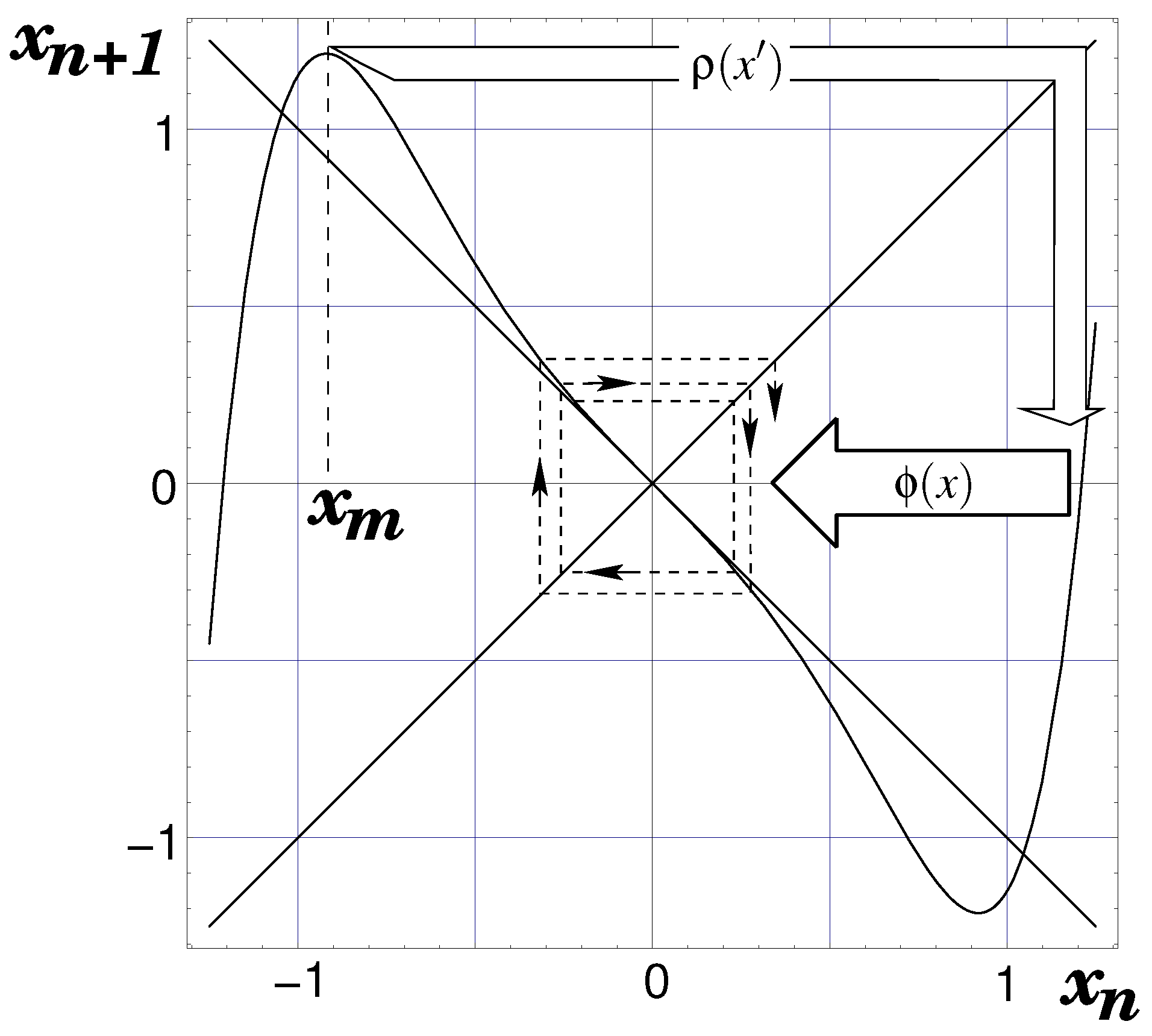
Figure 7.
Local map of Equation (141) for and its associated potential Equation (143). The potential barrier is also indicated. Reprinted from the book “New Advances on Chaotic Intermittency and its Applications,” authors Sergio Elaskar and Ezequiel del Rio, Copyright (2017) with permission from Springer Nature.

Figure 8.
Local map of Equation (154) for and its associated potential Equation (155). The potential barrier is also indicated. Reprinted from the book “New Advances on Chaotic Intermittency and its Applications,” authors Sergio Elaskar and Ezequiel del Rio, Copyright (2017) with permission from Springer Nature.

Figure 9.
Noisy map (183). The horizontal dashed line indicates the noiseless trajectory going into the laminar region. The nosily trajectory should be expanded to end inside the interval . Reprinted from the book “New Advances on Chaotic Intermittency and its Applications”, authors Sergio Elaskar and Ezequiel del Rio, Copyright (2017) with permission from Springer Nature.

Figure 10.
Map of Equation (189). Dashed arrows indicate the trajectory of a point near the maximum. Solid lines at both sides of the mentioned arrows indicate the effect of the noisy map on the same point, which will be mapped on the interval I over the graph of the map. Reprinted from the book “New Advances on Chaotic Intermittency and its Applications,” authors Sergio Elaskar and Ezequiel del Rio, Copyright (2017) with permission from Springer Nature.
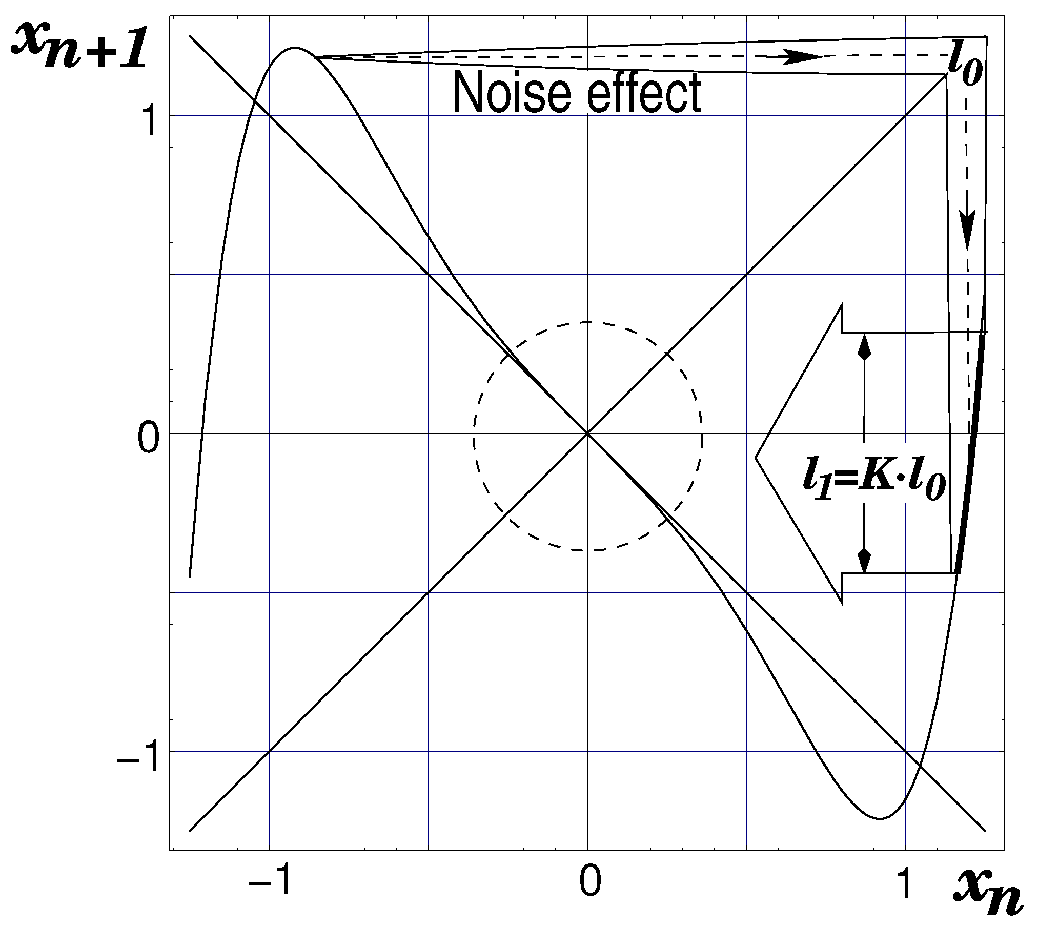
Figure 11.
NRPD corresponding to Equation (195) with . Dashed and solid lines show RPD and NRPD, respectively. Note that for , where .
Figure 11.
NRPD corresponding to Equation (195) with . Dashed and solid lines show RPD and NRPD, respectively. Note that for , where .

Figure 12.
Density evolution. Green arrows: Equation (215). Red arrows: Equation (214). Blue arrow: Equation (213).

Figure 13.
Reinjection process ruled by and functions.

Disclaimer/Publisher’s Note: The statements, opinions and data contained in all publications are solely those of the individual author(s) and contributor(s) and not of MDPI and/or the editor(s). MDPI and/or the editor(s) disclaim responsibility for any injury to people or property resulting from any ideas, methods, instructions or products referred to in the content. |
© 2023 by the authors. Licensee MDPI, Basel, Switzerland. This article is an open access article distributed under the terms and conditions of the Creative Commons Attribution (CC BY) license (https://creativecommons.org/licenses/by/4.0/).
Share and Cite
MDPI and ACS Style
Elaskar, S.; del Río, E. Review of Chaotic Intermittency. Symmetry 2023, 15, 1195. https://doi.org/10.3390/sym15061195
AMA Style
Elaskar S, del Río E. Review of Chaotic Intermittency. Symmetry. 2023; 15(6):1195. https://doi.org/10.3390/sym15061195
Chicago/Turabian StyleElaskar, Sergio, and Ezequiel del Río. 2023. "Review of Chaotic Intermittency" Symmetry 15, no. 6: 1195. https://doi.org/10.3390/sym15061195
Note that from the first issue of 2016, this journal uses article numbers instead of page numbers. See further details here.