The Analysis of Bifurcation, Quasi-Periodic and Solitons Patterns to the New Form of the Generalized q-Deformed Sinh-Gordon Equation

Abstract

In this manuscript, a new form of the generalized q-deformed Sinh-Gordon equation is investigated which could model physical systems with broken symmetries and to incorporate phenomena involving amplification or dissipation. The proposed model is explored based on the Lie symmetry approach. Using similarity reduction, the partial differential equation is transformed into an ordinary differential equation. By employing the generalized auxiliary equation approach, precise results for the derived equation are obtained. The solutions are graphically depicted as 3D, 2D, and contour plots. Furthermore, the qualitative analysis of the considered model is investigated by employing the concepts of bifurcation and chaos. The phase profiles are displayed for different sets of the parameters. Additionally, by applying an external periodic strength, quasi-periodic and chaotic behaviors are documented. Various tools for detecting chaos are discussed, including 3D and 2D phase patterns, time series, and Poincaré maps. Additionally, a sensitivity analysis is conducted for various initial conditions. The obtained findings are unique and indicate the viability and efficacy of the suggested strategies for evaluating soliton solutions and phase illustrations for various nonlinear models.

1. Introduction

In multiple scientific fields, nonlinear partial differential equations (NLPDEs) assist in modeling complicated phenomena that illustrate our day-to-day challenges. The usage of nonlinear models has proliferated in several disciplines, including demography [1], electromagnetic attraction in plasma [2], quantum science [3], and optics [4]. Identifying exact solutions of NLPDEs is a vital research discipline, since analytical solutions indicate the physical features of nonlinear systems [5,6]. Numerous effective approaches have been adopted to identify the analytical results for NLPDEs; some of them are the direct Ansatz approach [7], the direct Hirota method [8], the Painlevé approach [9], the modified auxiliary equation approach [10], and the Lie symmetry approach [11]. Among these methodologies, the Lie analysis technique is the most powerful and viable strategy for obtaining a precise solution to NLPDEs.

In the current work, the Lie symmetry approach [12,13] is employed to examine the investigated model. This idea was first introduced in the latter half of the nineteenth century by the mathematician Sophus Lie [14,15]. A Lie point symmetry is a one-parameter Lie group of transformations induced by a vector field that preserves the solution space of the equation. Each symmetry can be utilized to transform the partial differential equation (PDE) into an ordinary differential equation (ODE), thereby reducing the number of independent variables. Recently, many scholars have employed Lie analysis on different nonlinear models to obtain analytical solutions. Some notable examples include the works of Dorodnitsyn et al. [16], Jhangeer et al. [17], and Hussain et al. [18]. Numerous solutions have been discovered in the literature, including soliton solutions, trigonometric solutions, lump wave solutions, and more [19,20,21,22]. A soliton is a wave that preserves its form while moving at a fixed pace. The notion of optical solitons is particularly intriguing, as several nonlinear models possess soliton solutions. Some noteworthy examples are the Noyes Field model [21], Boussinesq equation [22], and Sine-Gordon equation [23,24].

The q-deformed equations serve a crucial role in the mathematical modeling of a variety of physical systems when they lose their symmetry [24,25,26]. Based on the premise of the q-deformed version of the Schrödinger equations, Q-bosons, black holes, the hydrogen atom, and the quantum harmonic oscillator were investigated [27,28,29]. The focus of this work is to explore the new form of the generalized q-deformed Sinh-Gordon equation in order to retrieve the analytical soliton solutions. The symmetry of the physical system is violated when the q-deformed function, as designed by Arai [30], becomes involved in the system. Symmetry breaking [31] is a basic phenomenon in particle physics. One of the most alluring and promising aspects of analyzing the discussed model is its potential in different fields, including quantum theory [32] and elasticity [33]. Eleuch [34] introduced a generalized form of the q-deformed model as follows:

$$\begin{array}{c}\hfill \frac{{\partial }^{2}u}{\partial r\partial s}=\alpha {[{\sinh }_q\left(u^{\beta }\right)]}^p-\delta ,\end{array}$$

(1)

where $\alpha$, $\beta$ and p are non-zero real constants, $\delta \in \mathbf{R}$ and $q\in (0,1]$.

Many scholars have examined the equation under evaluation in order to attain its analytical solutions. Raza et al. [35] employed $\exp (-\varphi (\xi \left)\right)$ and a generalized Riccati equation approach on the considered equation, extracting trigonometric and hyperbolic solutions. Ali and Abdel-Aty [36] solved the q-deformed equation analytically and numerically by utilizing an extended tanh methodology and a b-spline finite element technique, obtaining soliton solutions. Furthermore, Raza et al. [37] investigated Equation (1) using an extended generalized Kudryashov technique and an improved $\tan \left(\frac{\varphi }{2}\right)$ expansion approach to obtain new results.

In the current study, we deal with a new form of the generalized q-deformed Sinh-Gordon equation [38] as follows:

$$\begin{array}{c}\hfill \frac{{\partial }^{2}u}{\partial r\partial s}=e^{\alpha u}{[{\sinh }_q\left(u^{\beta }\right)]}^p-\delta ,\end{array}$$

(2)

where ${\sinh }_q$ is an Arai q-deformed function given as

$${\sinh }_q\left(u\right)=\frac{e^u-q{e}^{-u}}{2}.$$

For $q=1$, we obtain standard sinh functions.

This article aims to derive analytical solutions for the discussed model using the generalized auxiliary equation technique [39]. To our knowledge, Equation (2) has not been assessed by employing this technique in the previous literature. The suggested strategy has several advantages over previously explored methodologies since it offers results in a more generic and explicit form, including trigonometric, exponential, rational, and hyperbolic functions. The major goal of utilizing the similarity reduction approach is to attain the similarity variables. We transform the NLPDEs into certain nonlinear ODEs by applying these similarity factors. After that, we reveal some analytical solutions to these generated nonlinear ODEs. The findings are visually indicated for specific values of relevant parameters as 3D, contour, and 2D plots.

The analysis of differential equations (DEs) using chaos and bifurcation theory has become an esteemed field of research in recent years. These domains tend to be beneficial assets for comprehending any complex system regulated by DEs. A bifurcation is a qualitative change in the behavior of a dynamical system resulting from changing parameters. There are different schemes for bifurcation, such as the pitchfork, the period-doubling bifurcation, Hopf bifurcations, and saddle-node bifurcation. An intrinsic part of the study of DEs is the investigation of the complicated behavior of nonlinear waves and the exploration of chaos theory. The study of chaos is crucial in the twenty-first century. There are different strategies for spotting chaos. This analysis highlights the most useful ones, which are phase portraits, time analysis, and Poincaré maps.

To our knowledge, the chaotic and bifurcation analysis of the considered model has not been investigated in prior studies. Recently, Rafiq et al. [40] carried out a study of bifurcation and chaos for shallow water waves and also obtained multi-solitons. Lie and Huang [41] investigated the conformable Fokas–Lenells model by utilizing bifurcation and chaos theory, and Zhang et al. [42] conducted a bifurcation analysis on the modified FitzHugh–Nagumo neuron model and obtained new results. We also analyze the sensitivity of the considered model. Sensitivity analysis investigates how several uncertainties impact the overall uncertainty of the system in a mathematical model. A system is highly sensitive when minor changes in input result in drastic changes in the output of the system.

The layout of the article is as follows: The mathematical analysis of the model is discussed in Section 2. Section 3 deals with Lie symmetry analysis. In Section 4, symmetry reductions are given. Analytical solutions of the model under consideration are derived in Section 5, along with graphical representations. Bifurcation is addressed in Section 6. Section 7 deals with chaos theory, a sensitivity analysis of the considered model is presented in Section 8, and in Section 9, concluding remarks are given.

2. The Mathematical Analysis

By using the standard transformation of the form:

$$\begin{array}{c}\hfill x=cr+\frac{s}{c},\\ \hfill t=cr-\frac{s}{c},\end{array}$$

where c is an arbitrary parameter, Equation (2) is transformed into the following form:

$$\begin{array}{c}\hfill \frac{{\partial }^{2}u}{\partial x^2}-\frac{{\partial }^{2}u}{\partial t^2}=e^{\alpha u}{[{\sinh }_q\left(u^{\beta }\right)]}^p-\delta ,\end{array}$$

(3)

here, we will consider the case when $\alpha$ = $\beta$ = p = 1. Then Equation (3) can be written as

$$\begin{array}{c}\hfill \frac{{\partial }^{2}u}{\partial x^2}-\frac{{\partial }^{2}u}{\partial t^2}=e^u[{\sinh }_q\left(u\right)]-\delta .\end{array}$$

(4)

By employing the transformation

$$\phi =e^u,$$

and

$${\sinh }_q\left(u\right)=\frac{e^u-q{e}^{-u}}{2},{\cosh }_q\left(u\right)=\frac{e^u+q{e}^{-u}}{2}.$$

Equation (4) is converted into the following form:

$$2\phi ({\phi }_{xx}-{\phi }_{tt})-2({\phi }_x^2-{\phi }_t^2)-{\phi }^4+(q+2\delta ){\phi }^2=0.$$

(5)

In the next section, we will extract the Lie symmetries of Equation (5).

3. Lie Symmetry Analysis

Let us consider the one-parameter Lie group of infinitesimal transformations in $(x,t,\phi )$ given by

$$\begin{array}{c}\hfill x^{*}=x+\epsilon {\zeta }^1(x,t,\phi )+O\left({\epsilon }^2\right),\\ \hfill t^{*}=t+\epsilon {\zeta }^2(x,t,\phi )+O\left({\epsilon }^2\right),\\ \hfill {\phi }^{*}=\phi +\epsilon \tau (x,t,\phi )+O\left({\epsilon }^2\right),\end{array}$$

where group parameter $\epsilon \ll 1$ and ${\zeta }^1$, ${\zeta }^2$ and $\tau$ are coefficient functions. The vector field corresponding to the Lie group mentioned above may be represented as

$$\mathsf{V}={\zeta }^1(x,t,\phi )\frac{\partial }{\partial x}+{\zeta }^2(x,t,\phi )\frac{\partial }{\partial t}+\tau (x,t,\phi )\frac{\partial }{\partial \phi },$$

where the coefficient functions ${\zeta }^1(x,t,\phi )$, ${\zeta }^2(x,t,\phi )$ and $\tau (x,t,\phi )$ are to be evaluated later.

The invariance condition for Equation (5) with $\mathsf{V}$ becomes

$$P{r}^{\left(2\right)}\mathsf{V}(2\phi ({\phi }_{xx}-{\phi }_{tt})-2({\phi }_x^2-{\phi }_t^2)-{\phi }^4+(q+2\delta ){\phi }^2){\mid }_{Eq.5=0}=0,$$

(6)

where $P{r}^{\left(2\right)}\mathsf{V}$ is the second prolongation of $\mathsf{V}$ defined as

$$P{r}^{\left(2\right)}\mathsf{V}=\mathsf{V}+{\tau }^x\frac{\partial }{\partial {\phi }_x}+{\tau }^t\frac{\partial }{\partial {\phi }_t}+{\tau }^{xx}\frac{\partial }{\partial {\phi }_{xx}}+{\tau }^{tt}\frac{\partial }{\partial {\phi }_{tt}}+{\tau }^{xt}\frac{\partial }{\partial {\phi }_{xt}},$$

(7)

$$\left\{\begin{array}{c}{\tau }^x=D_x\left(\tau \right)-{\phi }_x{D}_x\left({\zeta }^1\right)-{\phi }_t{D}_x\left({\zeta }^2\right),\hfill \\ {\tau }^t=D_t\left(\tau \right)-{\phi }_x{D}_t\left({\zeta }^1\right)-{\phi }_t{D}_t\left({\zeta }^2\right),\hfill \\ {\tau }^{xx}=D_x\left({\tau }^x\right)-{\phi }_{xx}{D}_x\left({\zeta }^1\right)-{\phi }_{xt}{D}_x\left({\zeta }^2\right),\hfill \\ {\tau }^{tt}=D_t\left({\tau }^t\right)-{\phi }_{xt}{D}_t\left({\zeta }^1\right)-{\phi }_{tt}{D}_t\left({\zeta }^2\right),\hfill \\ {\tau }^{xt}=D_x\left({\tau }^t\right)-{\phi }_{xx}{D}_x\left({\zeta }^1\right)-{\phi }_{xt}{D}_x\left({\zeta }^2\right),\hfill \end{array}\right.$$

(8)

with $D_x$ and $D_t$ are total derivatives with respect to x and t, it can written as

$$D_i=\frac{\partial }{\partial x^i}+{\phi }_i\frac{\partial }{\partial \phi }+{\phi }_{ij}\frac{\partial }{\partial {\phi }_j}+...,i=1,2.$$

Plugging Equation (7) together with Equation (8) into Equation (6) yields the following system of determining equations:

$${\zeta }_{tt}^1=0,{\zeta }_x^2={\zeta }_t^1,{\zeta }_x^1={\zeta }_t^2={\zeta }_{\phi }^2={\zeta }_{\phi }^1={\tau }_{\phi }=0,$$

(9)

where ${\zeta }_{tt}=\frac{{\partial }^{2\zeta }}{\partial t^2}$,${\zeta }_x=\frac{\partial \zeta }{\partial x}$, ${\zeta }_t=\frac{\partial \zeta }{\partial t}$, ${\zeta }_{\phi }=\frac{\partial \zeta }{\partial \phi }$, ${\tau }_{\phi }=\frac{\partial \tau }{\partial \phi }$.

Solving above system (9) yields the symmetries for Equation (5) as follows:

$${\zeta }^1=C_{1}t+C_2,{\zeta }^2=C_{1}x+C_3,\tau =0,$$

(10)

where $C_i$, $i=1,2,3$ are constants. So, the infinitesimals of Equation (5) may be expresses as

$${\mathsf{V}}_1=\frac{\partial }{\partial x},{\mathsf{V}}_2=\frac{\partial }{\partial t},{\mathsf{V}}_3=t\frac{\partial }{\partial x}+x\frac{\partial }{\partial t}.$$

4. Symmetry Reductions

In this portion, we will reduce Equation (5) into corresponding ODEs by utilizing vector fields. For learning more about the Lie symmetry approach for differential equations, interested readers are directed to see [43,44].

Reduction using the symmetry •${\pounds }_1=\langle t{\mathsf{V}}_1+x{\mathsf{V}}_2\rangle$

The characteristic equation under this case can be expresses as

$$\frac{dx}{t}=\frac{dt}{x}=\frac{d\phi }{0}.$$

By integrating above equation, we acquire

$$\phi (x,t)=\chi \left(\eta \right),\mathrm{where}\eta =x^2-t^2.$$

(11)

By inserting Equation (11) into Equation (5), we obtain

$$8\eta \chi {\chi }^{″}-8\eta {\left({\chi }^{\prime }\right)}^2+8\chi {\chi }^{\prime }-{\chi }^4+(q+2\delta ){\chi }^2=0,$$

(12)

where ${}^{\prime }$ denotes the differentiation with respect to $\eta$.

Reduction using the translational symmetry•${\pounds }_2=\langle c_1{\mathsf{V}}_1+c_2{\mathsf{V}}_2\rangle$

The characteristic equation for this case is of the following form:

$$\frac{dx}{c_1}=\frac{dt}{c_2}=\frac{d\phi }{0}.$$

By integrating the above equation, we acquire

$$\phi (x,t)=\chi \left(\eta \right),\mathrm{where}\eta =c_{2}x-c_{1}t.$$

(13)

By inserting Equation (13) into Equation (5), we obtain

$$2(c_2^2-c_1^2)\chi {\chi }^{″}-2(c_2^2-c_1^2){\left({\chi }^{\prime }\right)}^2-{\chi }^4+(q+2\delta ){\chi }^2=0.$$

(14)

The next goal is to extract the traveling wave patterns for Equation (14) by employing the generalized auxiliary equation approach [39].

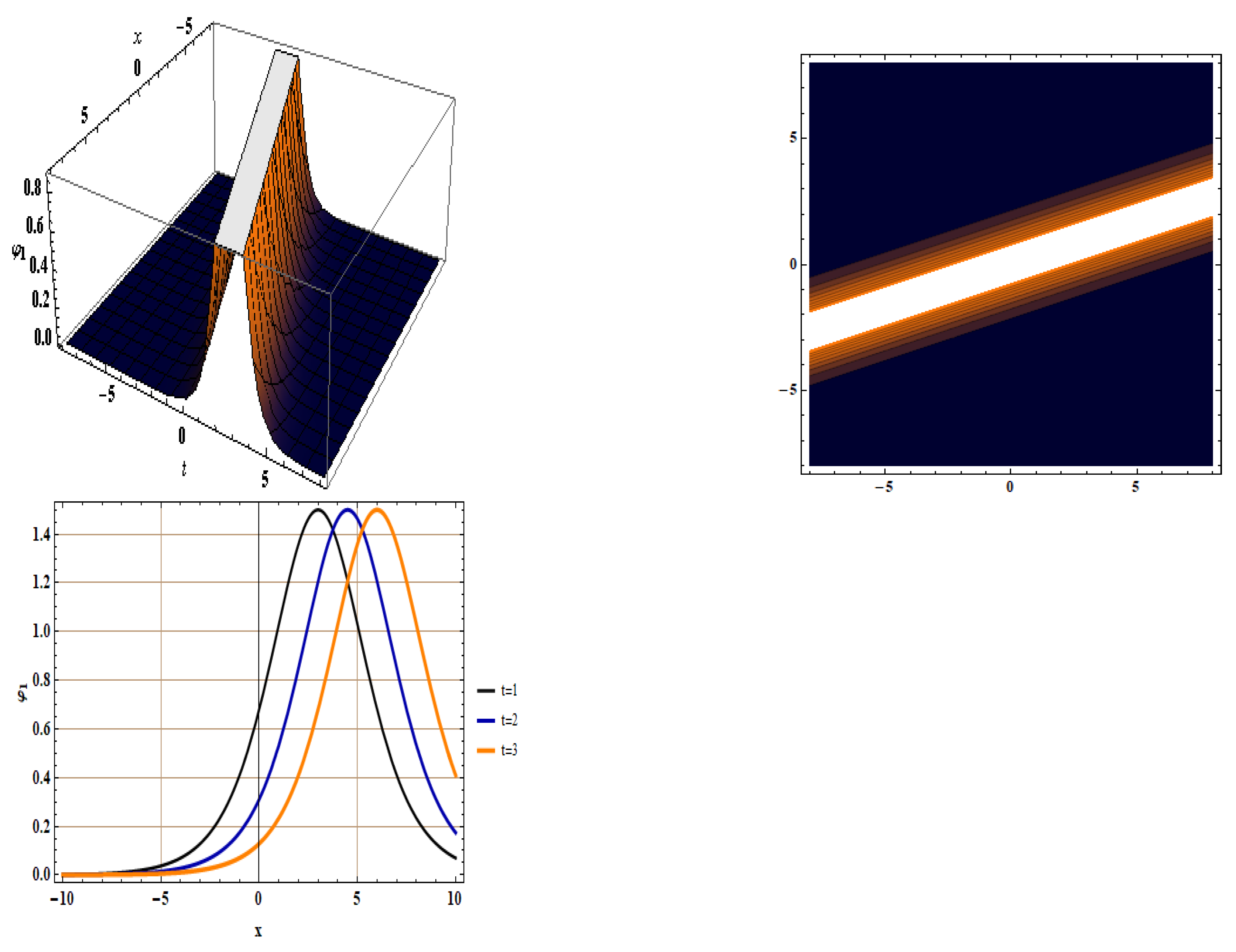
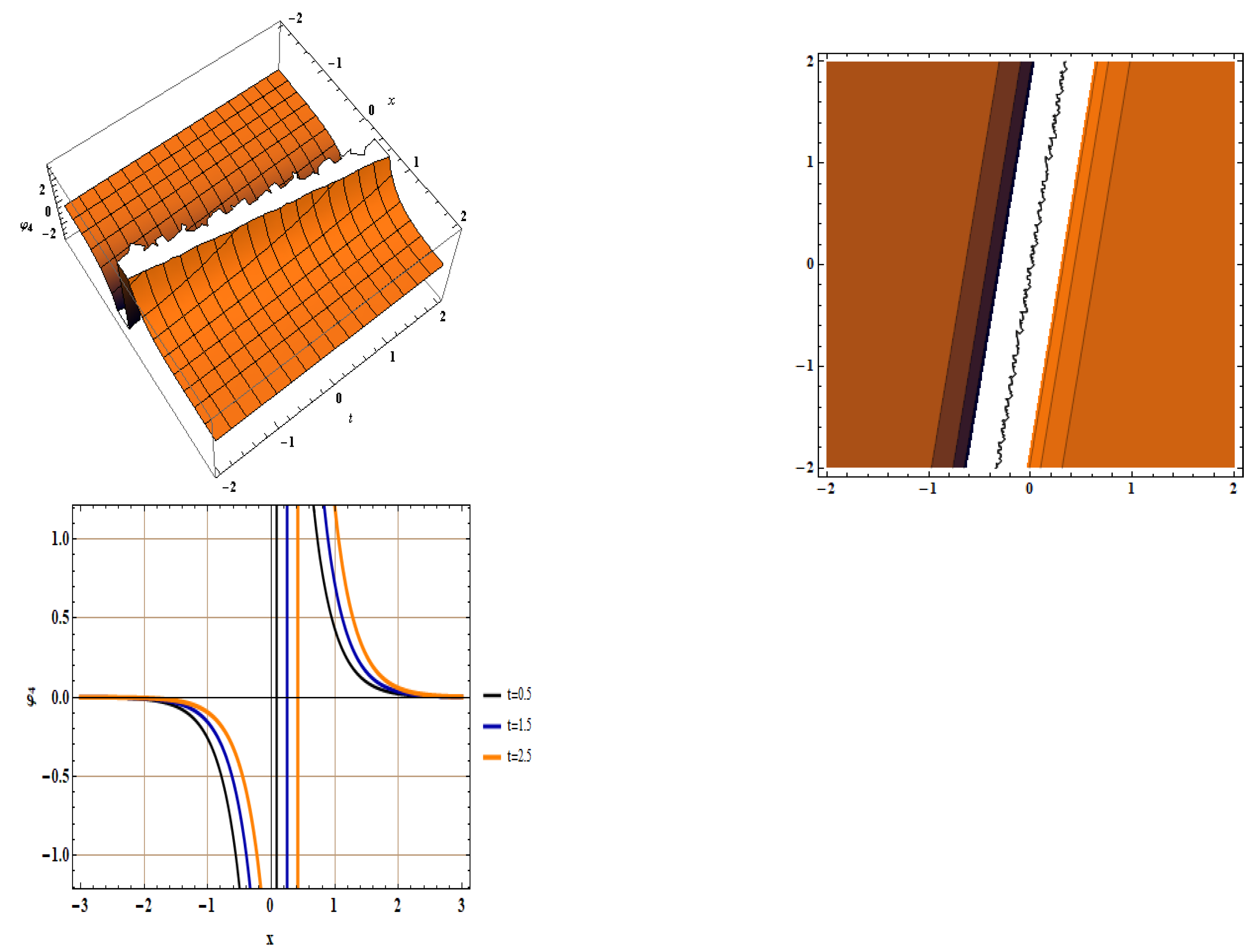
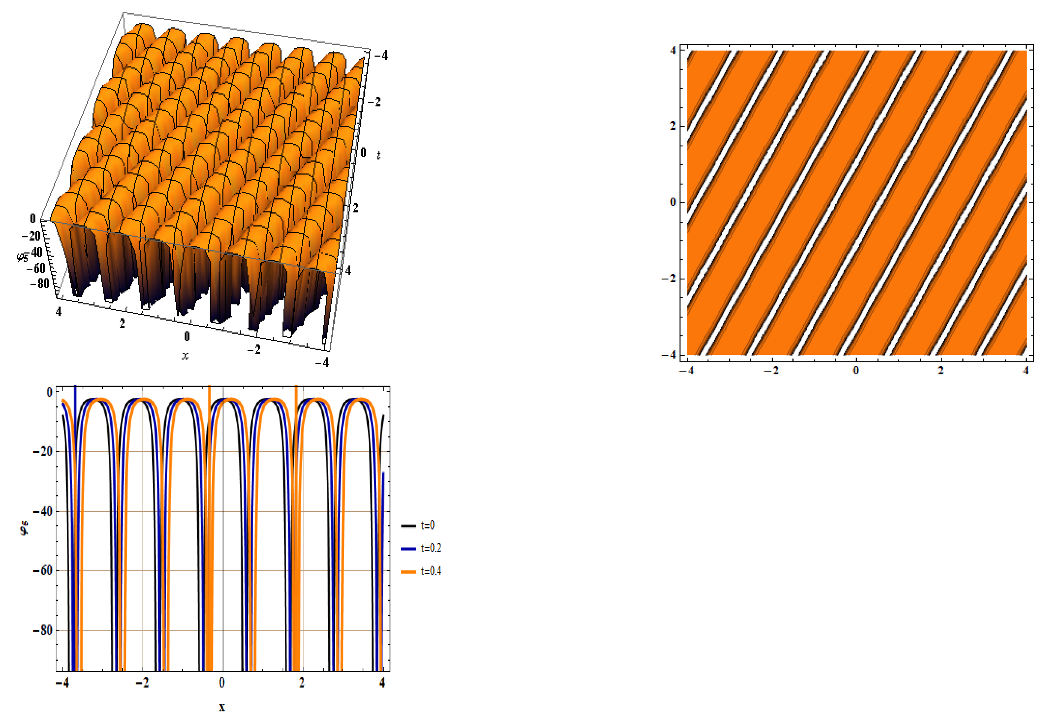
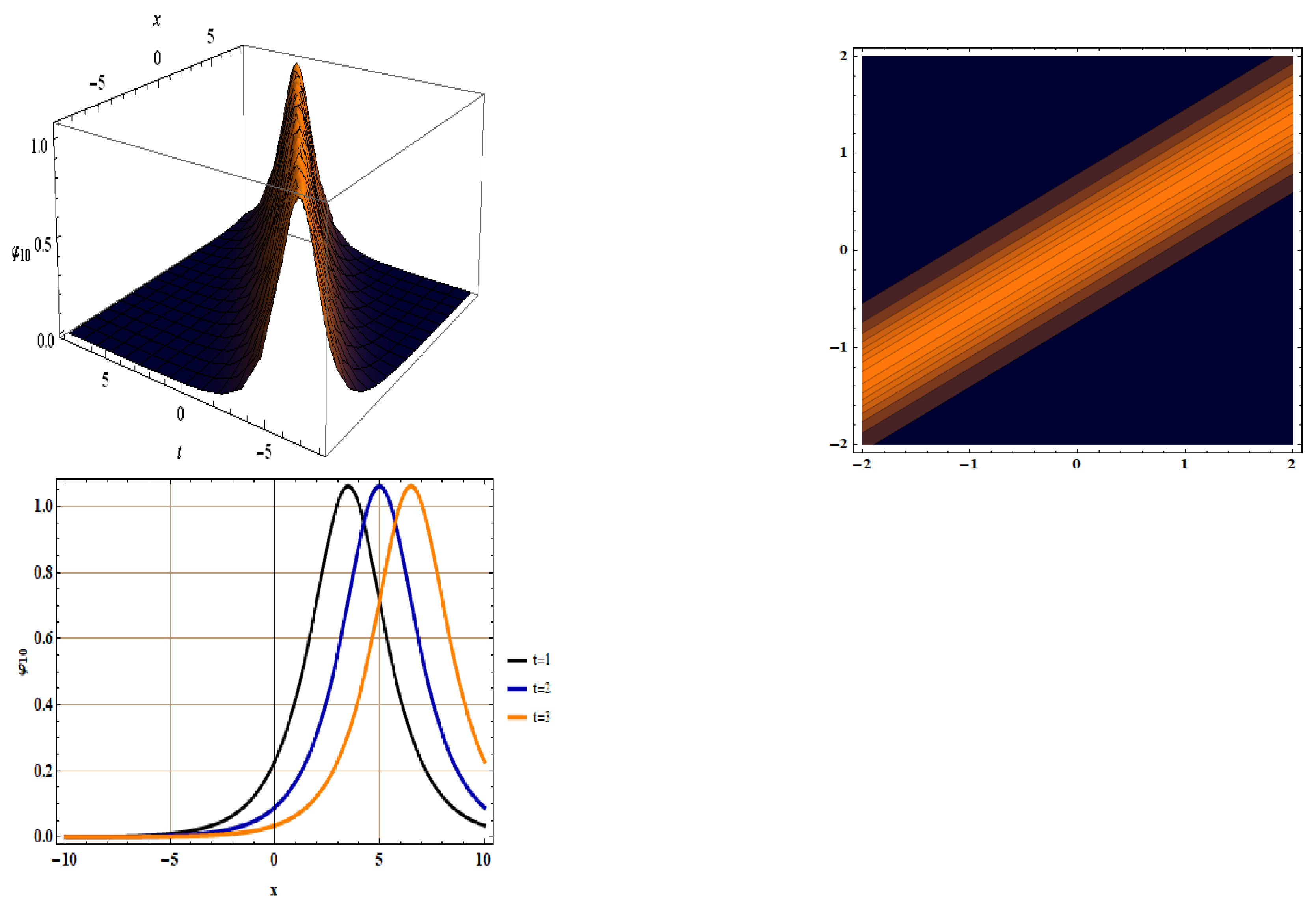
5. Soliton Solutions for Equation (5)

After turning PDE into ODEs in the preceding section, we will now obtain some analytical solutions to the resulting equation. Under present section, we will extract the traveling wave profiles of Equation (14) with the assistance of the generalized auxiliary equation approach. According to this methodology, the initial solution takes the following form:

$$\begin{array}{c}\hfill \chi \left(\eta \right)=\sum _{i=0}^M{w}_i{\mathsf{{\rm Y}}}^i\left(\eta \right),\end{array}$$

where the positive integer M can be evaluated by utilizing the homogeneous balance principle between the highest order derivative and the nonlinear term in the corresponding ODE. Balancing the terms $\chi {\chi }^{″}$ and ${\chi }^4$ in Equation (14) as $4M=M+M+2$ results in $M=1$. According to given technique for $M=1$, we make the following assumption about initial solution:

$$\chi \left(\eta \right)=w_0+w_1\mathsf{{\rm Y}}\left(\eta \right),$$

(15)

where $w_0$ and $w_1$ are arbitrary parameters to be evaluated later. Moreover, $\mathsf{{\rm Y}}=\mathsf{{\rm Y}}\left(\eta \right)$, satisfying the following ODE:

$${\mathsf{{\rm Y}}}^{\prime }=\sqrt{h_1{\mathsf{{\rm Y}}}^2+h_2{\mathsf{{\rm Y}}}^3+h_3{\mathsf{{\rm Y}}}^4}.$$

(16)

Here, $h_1$, $h_2$, and $h_3$ are real constants. Plugging Equations (15) and (16) into Equation (14) and reducing the coefficients of ${\mathsf{{\rm Y}}}^i$ to zero yields

$$\begin{array}{c}\hfill \left\{\begin{array}{c}{\mathsf{{\rm Y}}}^0:-{w_0}^4+\left(q+2\delta \right){w_0}^2=0,\hfill \\ {\mathsf{{\rm Y}}}^1:2\left(-{c_1}^2+{c_2}^2\right)w_0{w}_1{h}_1-4{w_0}^3{w}_1+2\left(q+2\delta \right)w_0{w}_1=0,\hfill \\ {\mathsf{{\rm Y}}}^2:3\left(-{c_1}^2+{c_2}^2\right)w_0{w}_1{h}_2-6{w_0}^2{w_1}^2+\left(q+2\delta \right){w_1}^2=0,\hfill \\ {\mathsf{{\rm Y}}}^3:4\left(-{c_1}^2+{c_2}^2\right)w_0{w}_1{h}_3+\left(-{c_1}^2+{c_2}^2\right){w_1}^2{h}_2-4w_0{w_1}^3=0,\hfill \\ {\mathsf{{\rm Y}}}^4:2\left(-{c_1}^2+{c_2}^2\right){w_1}^2{h}_3-{w_1}^4=0,\hfill \end{array}\right.\end{array}$$

after which, this system is solved for $w_0$, $w_1$, q, $\delta$, $h_1$, $h_2$, $h_3$, $c_1$, and $c_2$. With the aid of a mathematical tool such as Maple, the following solutions from above system can be determined.

$$\begin{array}{c}\hfill w_0=0,w_1=1.5,,h_2=0,h_3=-\frac{{w_1}^2}{2\left(c_1-c_2\right)\left(c_1+c_2\right)}.\end{array}$$

By plugging above values in Equation (15) and using the transformation given in Equation (13), the solutions of Equation (5) are obtained as follows,

• Type 1: For $h_1>0$ and $\mathsf{\Theta }=h_2^2-4h_1{h}_3>0$, we have

  $${\phi }_1(x,t)=1.5\left(\frac{2h_1{\mathrm{sech}}^2\left(\sqrt{h_1}\eta \right)}{\pm \sqrt{\mathsf{\Theta }}-h_2\mathrm{sech}\left(\sqrt{h_1}\eta \right)}\right).$$

  (17)

  $${\phi }_2(x,t)=1.5\left(\frac{2h_1{\mathrm{csch}}^2\left(\sqrt{h_1}\eta \right)}{\pm \sqrt{-\mathsf{\Theta }}-h_2\mathrm{csch}\left(\sqrt{h_1}\eta \right)}\right).$$

  (18)
• Type 2: For $h_1>0$ and $h_3>0$, we have

  $${\phi }_3(x,t)=1.5\left(\frac{-h_1{\mathrm{sech}}^2\left(\frac{\sqrt{h_1}}{2}\eta \right)}{h_2\pm 2\sqrt{h_1{h}_3}\tanh \left(\frac{\sqrt{h_1}}{2}\eta \right)}\right).$$

  (19)

  $${\phi }_4(x,t)=1.5\left(\frac{h_1{\mathrm{csch}}^2\left(\frac{\sqrt{h_1}}{2}\eta \right)}{h_2\pm 2\sqrt{h_1{h}_3}\coth \left(\frac{\sqrt{h_1}}{2}\eta \right)}\right).$$

  (20)
• Type 3: For $h_1<0$ and $\mathsf{\Theta }=h_2^2-4h_1{h}_3>0$, we have

  $${\phi }_5(x,t)=1.5\left(\frac{2h_1{\sec }^2\left(\sqrt{-h_1}\eta \right)}{\pm \sqrt{\mathsf{\Theta }}-h_2\sec \left(\sqrt{-h_1}\eta \right)}\right).$$

  (21)

  $${\phi }_6(x,t)=1.5\left(\frac{2h_1{\csc }^2\left(\sqrt{-h_1}\eta \right)}{\pm \sqrt{\mathsf{\Theta }}-h_2\csc \left(\sqrt{-h_1}\eta \right)}\right).$$

  (22)
• Type 4: For $h_1<0$ and $h_3>0$, we have

  $${\phi }_7(x,t)=1.5\left(\frac{-h_1{\sec }^2\left(\frac{\sqrt{-h_1}}{2}\eta \right)}{h_2\pm 2\sqrt{-h_1{h}_3}\tan \left(\frac{\sqrt{-h_1}}{2}\eta \right)}\right).$$

  (23)

  $${\phi }_8(x,t)=1.5\left(\frac{-h_1{\csc }^2\left(\frac{\sqrt{-h_1}}{2}\eta \right)}{h_2\pm 2\sqrt{-h_1{h}_3}\cot \left(\frac{\sqrt{-h_1}}{2}\eta \right)}\right).$$

  (24)
• Type 5: For $h_1>0$, we have

  $${\phi }_9(x,t)=1.5\left(\frac{4h_1{e}^{\pm \sqrt{h_1}\eta }}{{(e^{\pm \sqrt{h_1}\eta }-h_2)}^2-4h_1{h}_3}\right).$$

  (25)
• Type 6: For $h_1>0$ and $h_2=0$, we have

  $${\phi }_{10}(x,t)=1.5\left(\frac{\pm 4h_1{e}^{\pm \sqrt{h_1}\eta }}{1-4h_1{h}_3{e}^{\pm 2\sqrt{h_1}\eta }}\right).$$

  (26)
• Type 7: For $h_1=0$ and $h_2=0$, we have

  $${\phi }_{11}(x,t)=1.5\left(\pm \frac{1}{\sqrt{h_3}\eta }\right).$$

  (27)

  with $\eta =c_{2}x-c_{1}t$ and $\mathsf{\Theta }=h_2^2-4h_1{h}_3$.
• Bright solitons, singular solitons, and singular periodic solitons have been recorded for ${\phi }_1(x,t)$, ${\phi }_4(x,t)$, ${\phi }_5(x,t)$, and ${\phi }_{10}(x,t)$. The obtained results have been displayed in Figure 1, Figure 2, Figure 3 and Figure 4.

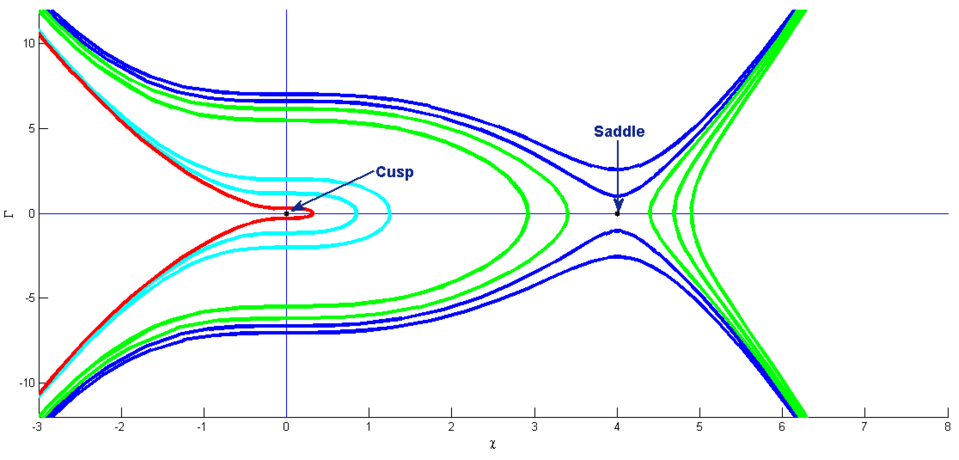
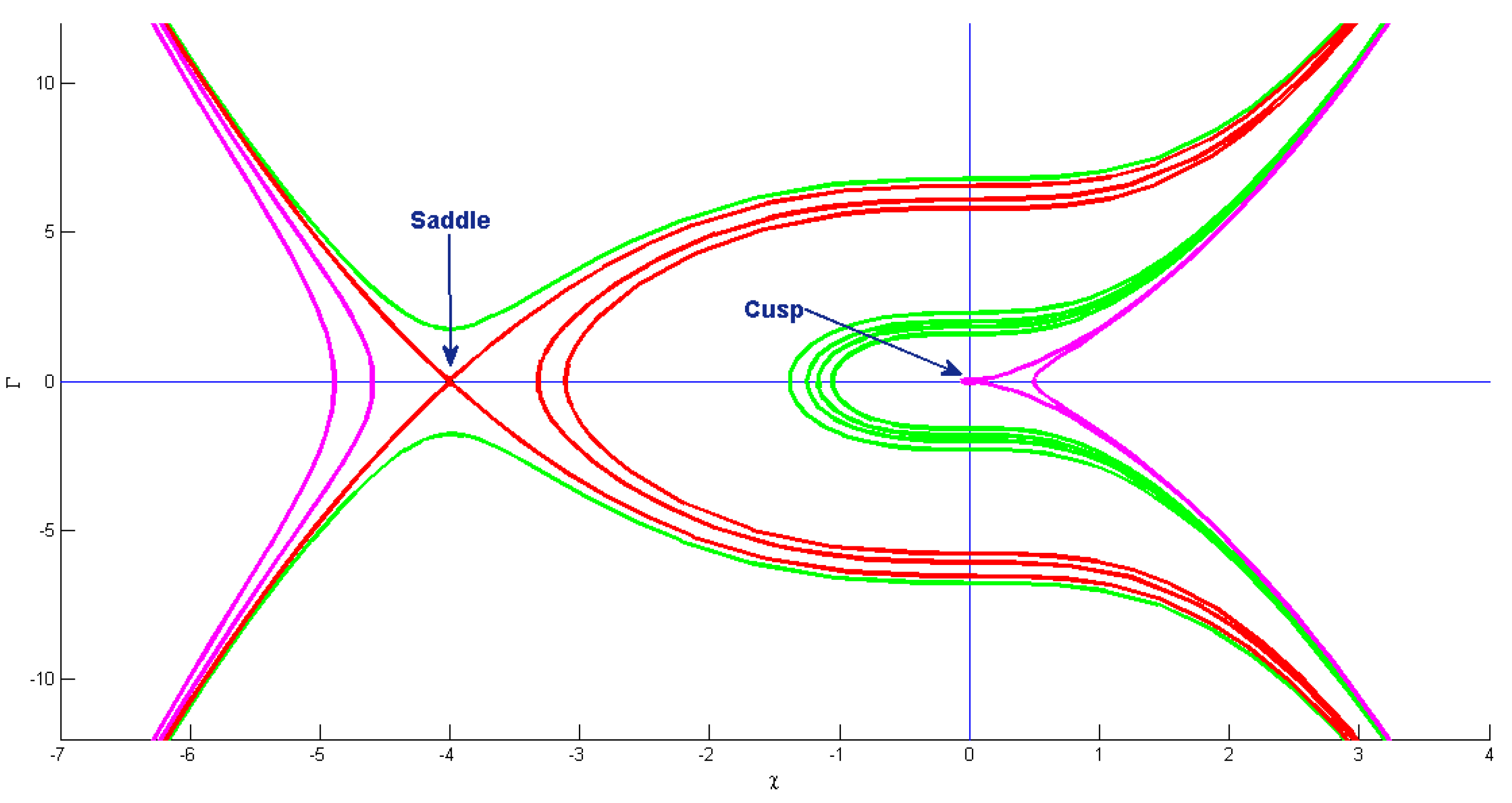
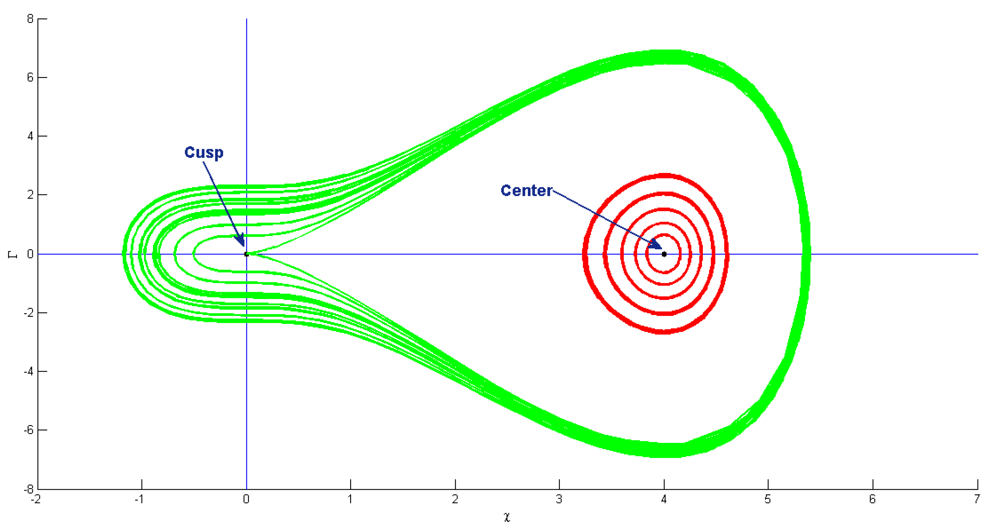
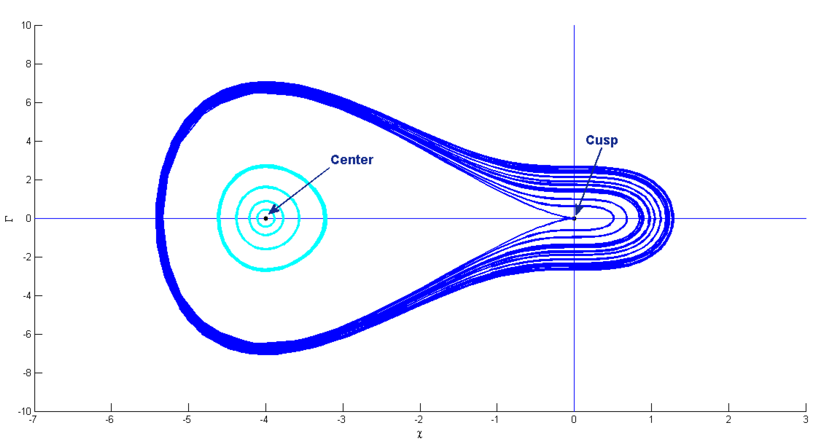
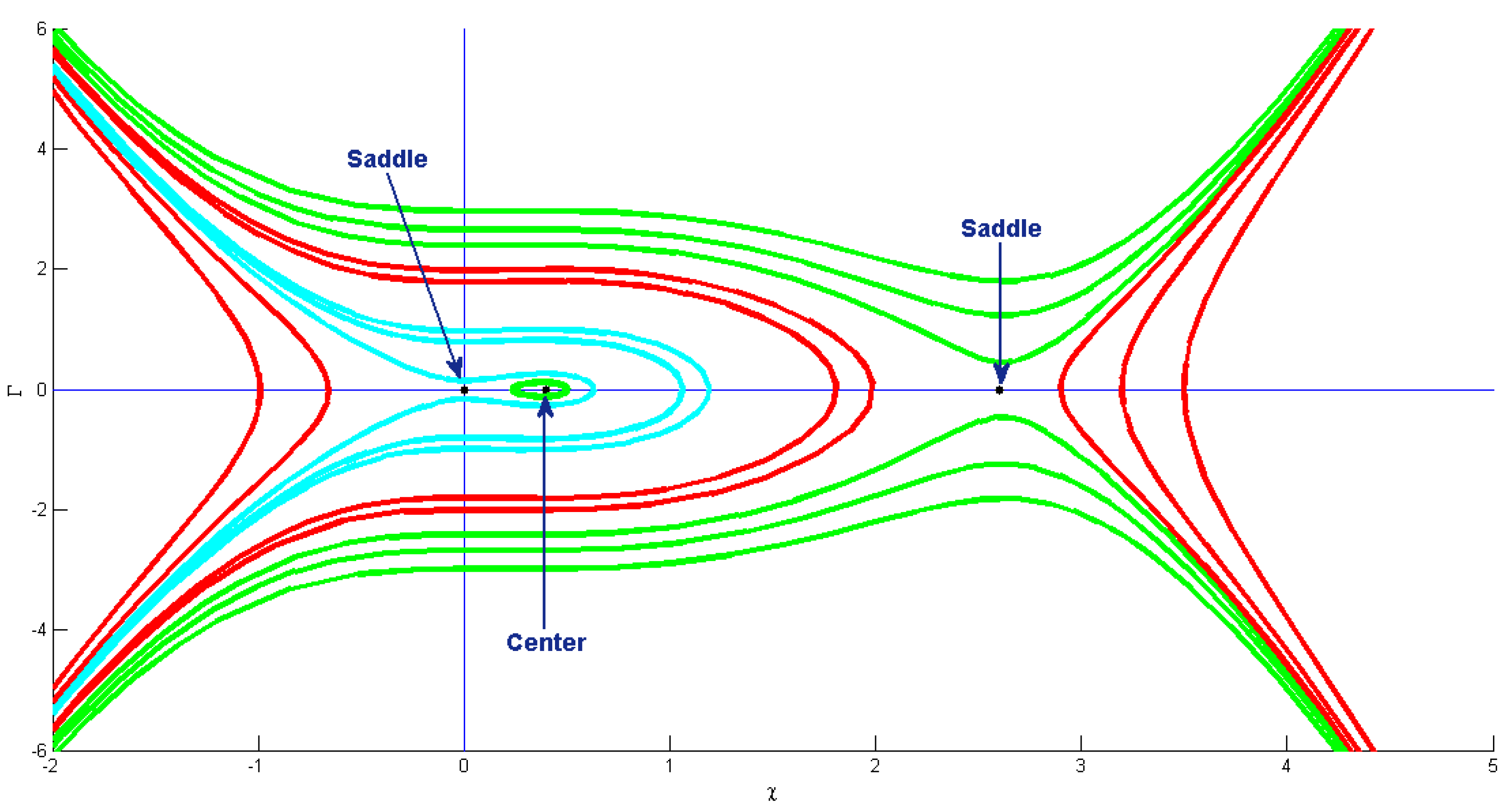
6. Bifurcation Analysis of Equation (5)

In this section, we examine Equation (2) using a bifurcation analysis. Using a Galilean transformation, Equation (14) can be transformed into a system of ordinary differential equations as

$$\left\{\begin{array}{c}\frac{d\chi }{d\eta }=\mathsf{\Gamma }\hfill \\ \frac{d\mathsf{\Gamma }}{d\eta }=\frac{2(c_2^2-c_1^2){\mathsf{\Gamma }}^2+{\chi }^4-(q+2\delta ){\chi }^2}{2(c_2^2-c_1^2)\chi },\hfill \end{array}\right.$$

(28)

which is not a Hamiltonian system, as it does not satisfy the Hamiltonian condition, that is,

$$\frac{d\chi }{d\eta }=\frac{\partial H}{\partial \mathsf{\Gamma }},\frac{d\mathsf{\Gamma }}{d\eta }=-\frac{\partial H}{\partial \chi }.$$

Here H represents the Hamiltonian. Using Equation (28), we obtain

$$\frac{d{\mathsf{\Gamma }}^2}{d\chi }=\frac{2(c_2^2-c_1^2){\mathsf{\Gamma }}^2+{\chi }^4-(q+2\delta ){\chi }^2}{(c_2^2-c_1^2)\chi },$$

(29)

where $\chi =0$ is a singular point of Equation (29). The solution for Equation (29) has the following form:

$${\mathsf{\Gamma }}^2={\chi }^{2}c+\frac{1}{2(c_1^2-c_2^2)}[4\delta \ln \left(\chi \right){\chi }^2+2q{\chi }^2\ln \left(\chi \right)-{\chi }^4],$$

(30)

where c is the constant of integration, we obtain

$${\left({\chi }^{\prime }\right)}^2-[{\chi }^{2}c+\frac{1}{2(c_1^2-c_2^2)}[4\delta \ln \left(\chi \right){\chi }^2+2q{\chi }^2\ln \left(\chi \right)-{\chi }^4]]=0.$$

(31)

Equation (31) can be expressed as

$$L(\chi ,\mathsf{\Gamma })={\mathsf{\Gamma }}^2-[{\chi }^{2}c+\frac{1}{2(c_1^2-c_2^2)}[4\delta \ln \left(\chi \right){\chi }^2+2q{\chi }^2\ln \left(\chi \right)-{\chi }^4]]=0,$$

(32)

which is a required conserved quantity. Furthermore, we perform a qualitative analysis of the above equation through utilizing the entire discrimination system. For this, consider the Equation (32) with its potential energy as

$$\begin{array}{c}\hfill W\left(\chi \right)=-[{\chi }^{2}c+\frac{1}{2(c_1^2-c_2^2)}[4\delta \ln \left(\chi \right){\chi }^2+2q{\chi }^2\ln \left(\chi \right)-{\chi }^4]]=0,\end{array}$$

further taking the derivative of the above equation; after some simplification, we have

$$W^{\prime }\left(\chi \right)=(-2c-\frac{2\delta }{(c_1^2-c_2^2)}-\frac{q}{(c_1^2-c_2^2)})\chi +\frac{2}{(c_1^2-c_2^2)}{\chi }^3-\frac{4\delta +2q}{(c_1^2-c_2^2)}\chi \ln \chi .$$

(33)

Employing the Taylor expansion of $\ln \left(\chi \right)$ around $\chi =0$, neglecting higher terms, yields

$$W^{\prime }\left(\chi \right)={\varrho }_1{\chi }^3-{\varrho }_2{\chi }^2+{\varrho }_3\chi ,$$

(34)

where ${\varrho }_1=\frac{2}{(c_1^2-c_2^2)}$, ${\varrho }_2=\frac{4\delta +2q}{(c_1^2-c_2^2)}$, and ${\varrho }_3=(-2c+\frac{2\delta }{(c_1^2-c_2^2)}+\frac{q}{(c_1^2-c_2^2)})$. By denoting

$$J(\chi ,\mathsf{\Gamma })=\left|\begin{array}{cc}0& 1\\ {\varrho }_3-2{\varrho }_2\chi +3{\varrho }_1{\chi }^2& 0\end{array}\right|$$

$$=-({\varrho }_3-2{\varrho }_2\chi +3{\varrho }_1{\chi }^2),$$

the eigenvalues on the singular point are

$${\lambda }_{\pm }(\chi ,\mathsf{\Gamma })=\pm \sqrt{({\varrho }_3-2{\varrho }_2\chi +3{\varrho }_1{\chi }^2)},$$

(35)

thus, $(\chi ,\mathsf{\Gamma })$ is a saddle point for $J(\chi ,\mathsf{\Gamma })<0$, a center for $J(\chi ,\mathsf{\Gamma })>0$, and a cusp for $J(\chi ,\mathsf{\Gamma })=0$.

The third order discriminant for the polynomial is

$$\mathsf{\Delta }={\varrho }_2^2{\varrho }_3^2-4{\varrho }_1{\varrho }_3^3,$$

(36)

and we obtain the following results that are shown below.

Case 1: Let $\mathsf{\Delta }=0$ and ${\varrho }_1>0$, ${\varrho }_2>0$ and ${\varrho }_3=0$, then

$$W^{\prime }\left(\chi \right)={\varrho }_1{(\chi -\mathit{j})}^2(\chi -\kappa ).$$

(37)

In this case, we obtain two points, $(\mathit{j},0)$, and $(\kappa ,0)$, as critical points. Considering such a case, $(\mathit{j},0)$ is the cusp and $(\kappa ,0)$ is the saddle point. By choosing $c_1=2$, $c_2=1.4$, ${\varrho }_1=1$, ${\varrho }_2=4$, ${\varrho }_3=0$, $\delta =2$, $q=0$, and $c=1$, we obtain $\mathit{j}=0$ and $\kappa =4$. These points are displayed in Figure 5.

Case 2: Let $\mathsf{\Delta }=0$ and ${\varrho }_1>0$, ${\varrho }_2<0$ and ${\varrho }_3=0$, then

$$W^{\prime }\left(\chi \right)={\varrho }_1{(\chi -\mathit{j})}^2(\chi -\kappa ).$$

(38)

In the present case, we have two points, $(\mathit{j},0)$ and $(\kappa ,0)$, as equilibrium points. Considering such a case $(\mathit{j},0)$ is the cusp and $(\kappa ,0)$ is the saddle point. By selecting $c_1=2$, $c_2=1.4$, ${\varrho }_1=1$, ${\varrho }_2=-4$, ${\varrho }_3=0$, $\delta =2$, $q=-8$, and $c=-1$, we obtain $\mathit{j}=0$ and $\kappa =-4$. These points are shown in Figure 6.

Case 3: Let $\mathsf{\Delta }=0$ and ${\varrho }_1<0$, ${\varrho }_2<0$ and ${\varrho }_3=0$, then

$$W^{\prime }\left(\chi \right)={\varrho }_1{(\chi -\mathit{j})}^2(\chi -\kappa ).$$

(39)

In the present case, two points, $(\mathit{j},0)$ and $(\kappa ,0)$, are critical points. Taking such a case, $(\mathit{j},0)$ is the cusp and $(\kappa ,0)$ is the central point. By fixing $c_2=2$, $c_1=1.4$, ${\varrho }_1=-1$, ${\varrho }_2=-4$, ${\varrho }_3=0$, $\delta =2$, $q=0$, and $c=-1$, we obtain $\mathit{j}=0$ and $\kappa =4$. These points are displayed in Figure 7.

Case 4: Let $\mathsf{\Delta }=0$ and ${\varrho }_1<0$, ${\varrho }_2>0$ and ${\varrho }_3=0$, then

$$W^{\prime }\left(\chi \right)={\varrho }_1{(\chi -\mathit{j})}^2(\chi -\kappa ).$$

(40)

In this case, we acquire $(\mathit{j},0)$ and $(\kappa ,0)$ as critical points. Considering this case, $(\mathit{j},0)$ is the cuspidal point and $(\kappa ,0)$ is the central point. By choosing $c_2=2$, $c_1=1.4$, ${\varrho }_1=-1$, ${\varrho }_2=4$, ${\varrho }_3=0$, $\delta =-2$, $q=0$ and $c=1$, we obtain $\mathit{j}=0$, and $\kappa =-4$. These points are presented in Figure 8.

Case 5: Let $\mathsf{\Delta }>0$ and ${\varrho }_1>0$, ${\varrho }_2>0$, ${\varrho }_3>0$ then

$$W^{\prime }\left(\chi \right)={\varrho }_1(\chi -\mathit{j})(\chi -\kappa )(\chi -\mathit{\ell }).$$

(41)

In this case, we acquire three points, $(\mathit{j},0)$, $(\kappa ,0)$, and $(\mathit{\ell },0)$, as equilibrium points. Considering such a case, $(\mathit{j},0)$ and $(\kappa ,0)$ are the saddle points, while $(\mathit{\ell },0)$ is the central point. By choosing $c_2=1.4$, $c_1=2$, ${\varrho }_1=1$, ${\varrho }_2=3$, ${\varrho }_3=1$, $\delta =0$, $q=3$, and $c=1$, we obtain $\mathit{j}=0$, $\kappa =2.6$ and $\mathit{\ell }=0.4$. These points are depicted in Figure 9.

Case 6: Let $\mathsf{\Delta }>0$ and ${\varrho }_1<0$, ${\varrho }_2=0$, ${\varrho }_3>0$, then

$$W^{\prime }\left(\chi \right)={\varrho }_1(\chi -\mathit{j})(\chi -\kappa )(\chi -\mathit{\ell }).$$

(42)

In this case, we obtain $(\mathit{j},0)$, $(\kappa ,0)$, and $(\mathit{\ell },0)$ as critical points. Taking such a case, $(\mathit{\ell },0)$ and $(\kappa ,0)$ are the central points, while $(\mathit{j},0)$ is the saddle point. By putting $c_2=2$, $c_1=1.4$, ${\varrho }_1=-1$, ${\varrho }_2=0$, ${\varrho }_3=1$, $\delta =0$, $q=0$, and $c=-0.5$, we obtain $\mathit{j}=0$, $\kappa =1$ and $\mathit{\ell }=-1$. These points are displayed in Figure 10.

Case 7: Let $\mathsf{\Delta }<0$ and ${\varrho }_1>0$, ${\varrho }_2>0$ and ${\varrho }_3>0$, then

$$W^{\prime }\left(\chi \right)={\varrho }_1(\chi -\mathit{j})[{(\chi -\kappa )}^2+{\mathit{\ell }}^2].$$

(43)

In present case, we acquire only one point, $(\mathit{j},0)$, as a critical point. It can be the center for ${\varrho }_3<0$ and the saddle for ${\varrho }_3>0$.

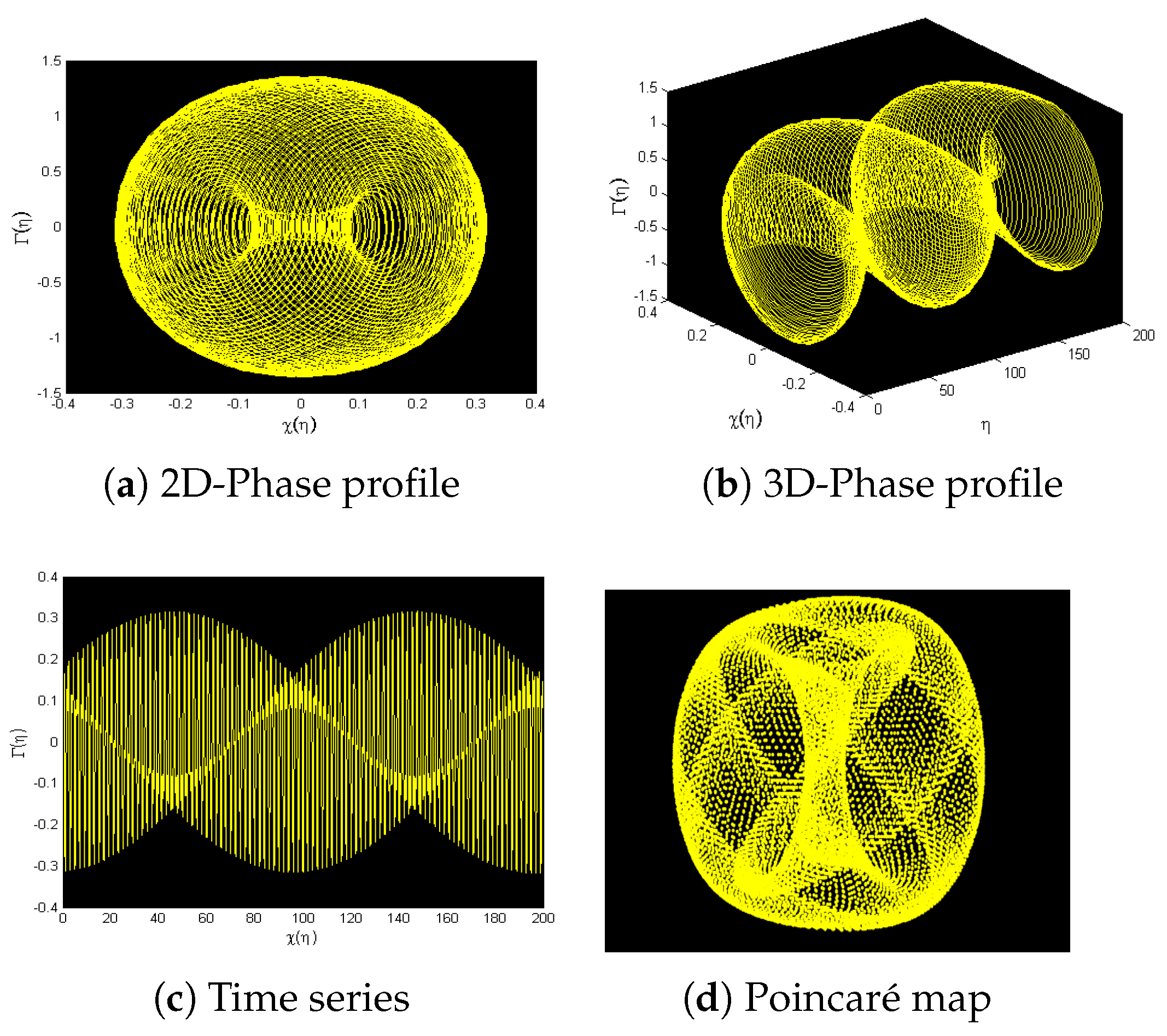
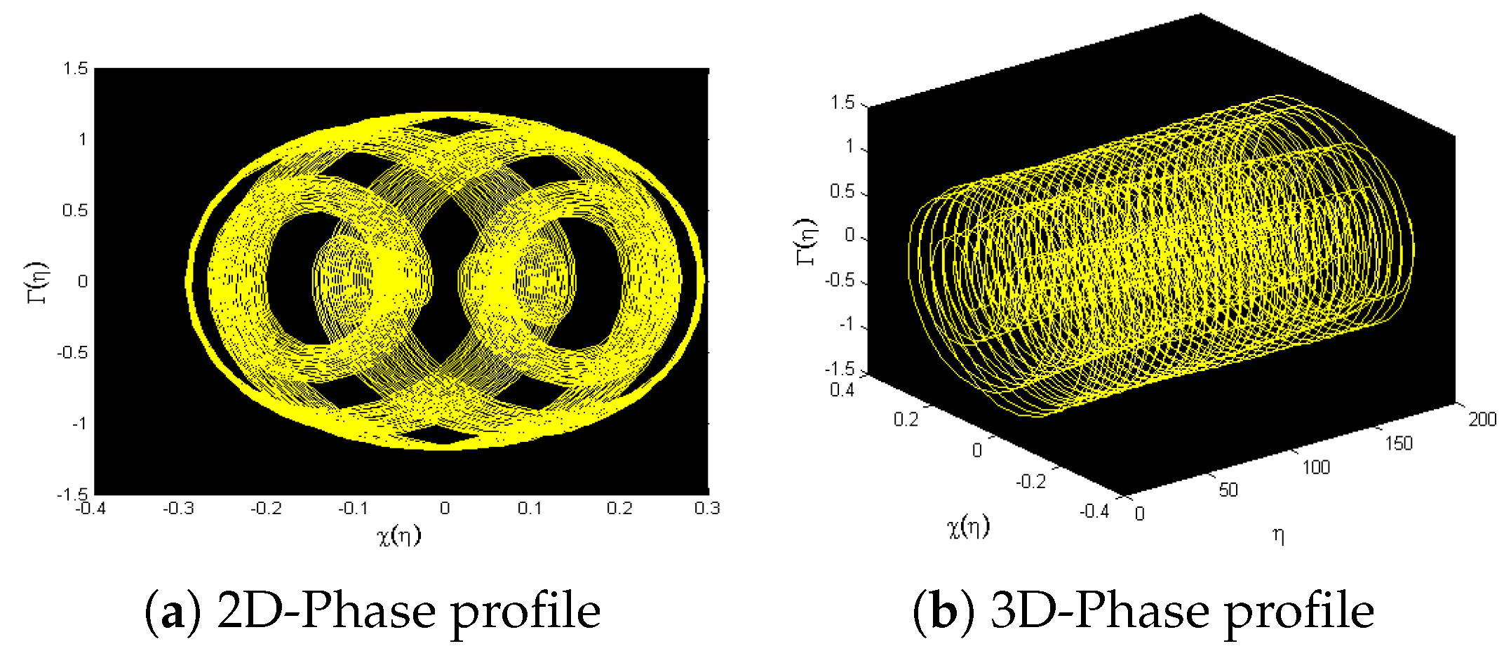
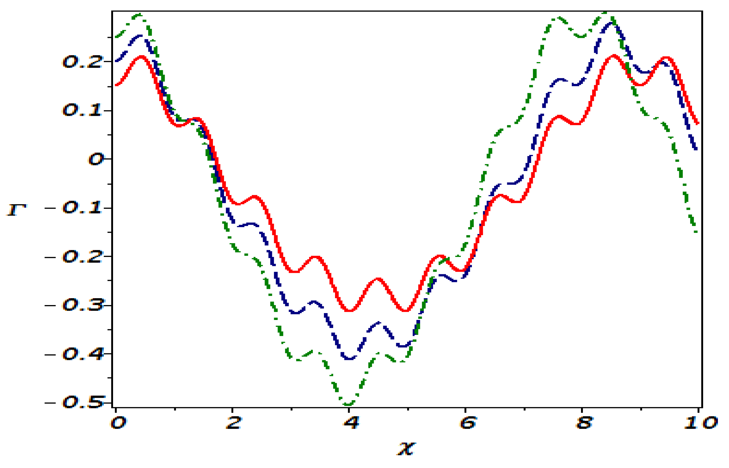
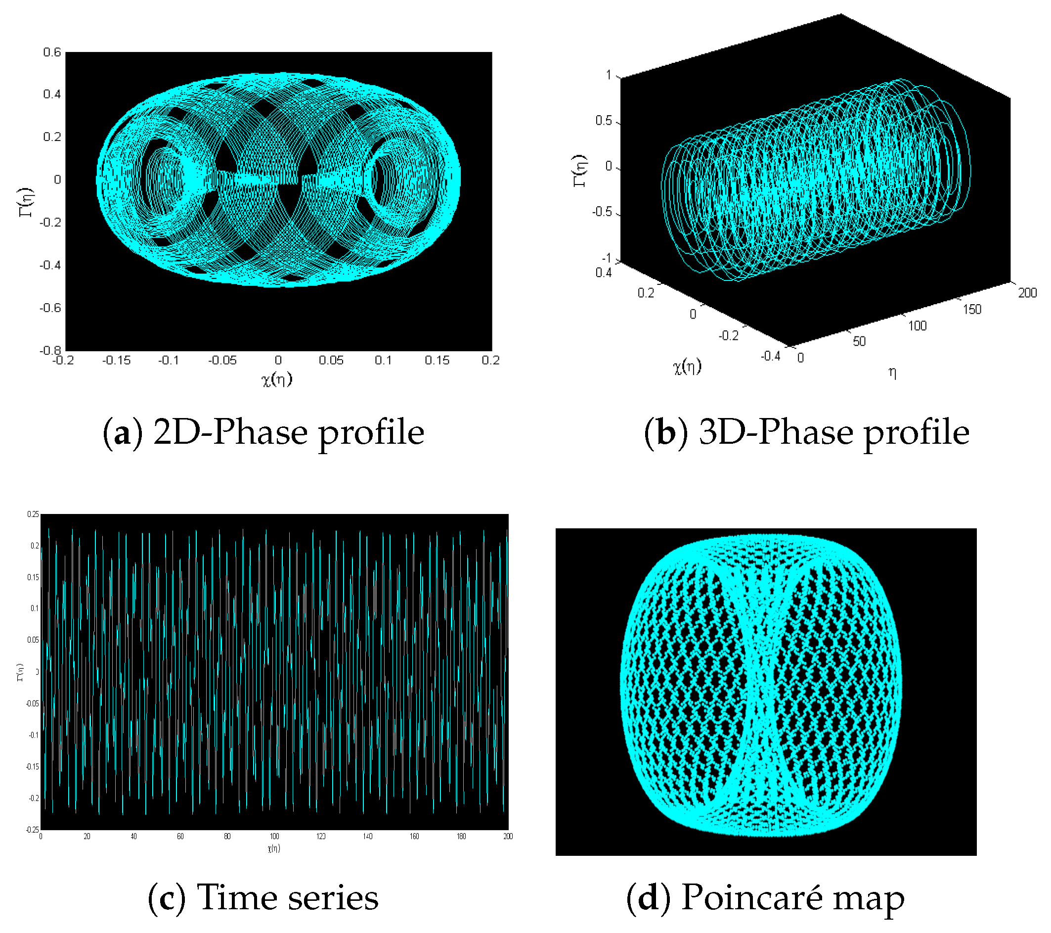
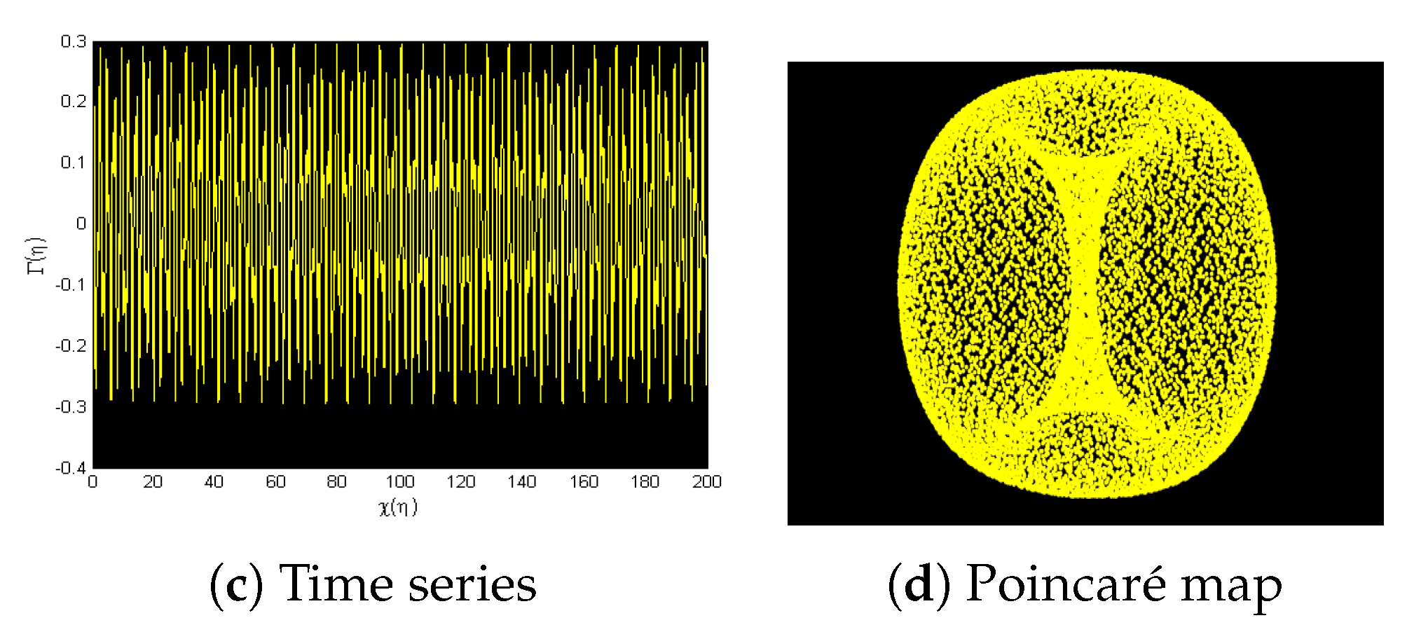
7. Phase Patterns for Quasi-Periodic Behavior

In this section, we analyze the quasi-periodic patterns of the perturbed system as follows:

$$\left\{\begin{array}{c}\frac{d\chi }{d\eta }=\mathsf{\Gamma }\hfill \\ \frac{d\mathsf{\Gamma }}{d\eta }={\varrho }_1{\chi }^3-{\varrho }_2{\chi }^2+{\varrho }_3\chi +{\rho }_0\cos \left(\kappa \eta \right),\hfill \end{array}\right.$$

(44)

where ${\varrho }_1=\frac{2}{(c_1^2-c_2^2)}$, ${\varrho }_2=\frac{4\delta +2q}{(c_1^2-c_2^2)}$ and ${\varrho }_3=(-2c+\frac{2\delta }{(c_1^2-c_2^2)}+\frac{q}{(c_1^2-c_2^2)})$.

Here, in the above system (44), ${\rho }_0$ represents the strength of the disruption and $\kappa$ represents the frequency. System (44) has an external periodic force of ${\rho }_0\cos \left(\kappa \eta \right)$, which is missing in system (28), to inspect the chaotic and periodic patterns of Equation (2). To tackle this issue, we employ a variety of tools, including the phase portrait approach, time series profiling, and Poincaré maps. To analyze the problem from different perspectives, we will assess the impact of the parameters ${\varrho }_1$, ${\varrho }_2$, ${\varrho }_3$, ${\rho }_0$, and $\kappa$ by assuming two alternate scenarios. In the first scenario, we will keep ${\varrho }_1$, ${\varrho }_2$, ${\varrho }_3$, and $\kappa$ constant and examine the impact of ${\rho }_0$. In the second case, we will investigate the effect of modifying the other factors while considering ${\rho }_0$ and $\phi$ as constants.

In Figure 11, 3D and 2D phase plots, time analysis graphs, and Poincaré maps are depicted for ${\varrho }_1=-3$, ${\varrho }_2=1.5$, ${\varrho }_3=-0.5$, ${\rho }_0=1.5$, and $\kappa =2\pi$. It is observed that system (44) exhibits quasi-periodic behavior for ${\rho }_0=1.5$. Figure 12 presents 3D and 2D plots along with time analysis graphs and Poincaré maps for ${\rho }_0=2.5$, while keeping the other factors the same as in Figure 11. System (44) appears to display quasi-periodic characteristics for ${\rho }_0=2.5$. In Figure 13, 3D and 2D plots, time series profiles, and Poincaré maps are shown for ${\varrho }_1=-3.5$, ${\varrho }_2=4$, ${\varrho }_3=-1.5$, ${\rho }_0=3.5$, and $\kappa =2\pi$. It is observed that system (44) exhibits quasi-periodic characteristics, while the Poincaré section has several disordered points indicating chaotic motion for the given parameters. In Figure 14, 3D and 2D plots, time series profiles, and Poincaré maps are displayed for ${\varrho }_1=-5.5$, ${\varrho }_2=2.5$, ${\varrho }_3=-2$, ${\rho }_0=3.5$, and $\kappa =2\pi$. It is noted that system (44) demonstrates a quasi-periodic pattern, while the Poincaré map shows many irregular points and depicts chaotic behavior.

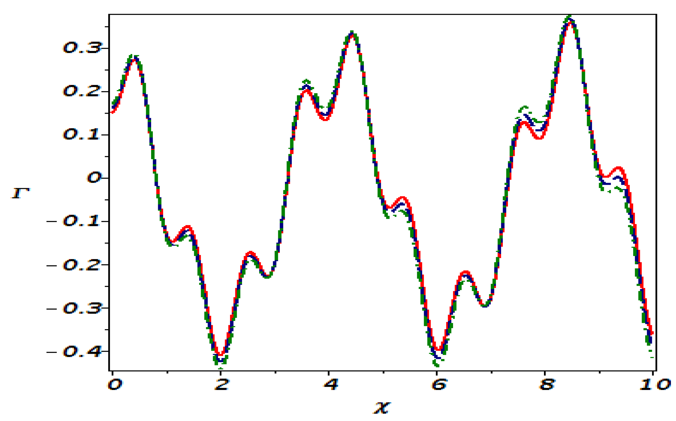
8. Sensitivity Analysis

Here, we have the sensitivity of the disturbed system (44). For this objective, we have taken into consideration three distinct initial conditions: $(\chi ,\mathsf{\Gamma })=(0.15,0)$, identified by the red solid line, $(\chi ,\mathsf{\Gamma })=(0.16,0)$, plotted with the blue dotted curve, and $(\chi ,\mathsf{\Gamma })=(0.17,0)$, shown by the green dotted curve. In Figure 15 and Figure 16, three solutions are addressed by considering the same values of parameters as those considered in Figure 11 and Figure 14. In Figure 17 and Figure 18, we make a tiny adjustment in the initial values, and the solutions are attained by choosing the same values for the parameters as in Figure 11 and Figure 14. It is indicated that a slight modification in initial conditions has no major impact on the solution. As a consequence, we conclude that the proposed model is not very sensitive.

9. Concluding Remarks

In this paper, we have investigated a new form of the generalized q-deformed Sinh-Gordon equation. The proposed model has been explored through a Lie symmetry analysis, where we have calculated the Lie point symmetries using the Lie group’s invariance criterion. By employing similarity reduction, we have transformed the partial differential equation (PDE) into an ordinary differential equation (ODE). Using the generalized auxiliary equation approach, we have generated a range of soliton profiles for the derived ODEs, considering various values of the parameters. The collected data are presented in the form of 2D, 3D, and contour graphical patterns. Based on our analysis, we have obtained the following results for the proposed model.

In Figure 1, we extracted bright solitons for ${\phi }_1$ by setting $h_1=1$, $h_2=0$, $h_3=0.2$, $c_1=0.5$, and $c_2=3$. Singular solitons for ${\phi }_4(x,t)$ were indicated in Figure 2, using the same parameter values. In Figure 3, we detected singular periodic solitons for ${\phi }_5(x,t)$ with $h_1=-2.1$, $h_2=0$, $h_3=0.75$, $c_1=1$, and $c_2=2$. Figure 4 shows the detection of bright solitons for ${\phi }_{10}(x,t)$ with $h_1=0.1$, $h_2=0$, $h_3=-0.2$, $c_1=3$, and $c_2=2$.

Furthermore, we have conducted a qualitative analysis of the model by investigating bifurcation and chaos. We have transformed the model into a dynamical system using the Galilean transformation and performed a bifurcation analysis. Phase profiles for different parameter scenarios are displayed in Figure 5, Figure 6, Figure 7, Figure 8, Figure 9 and Figure 10. Additionally, by introducing an external periodic strength, we have observed quasi-periodic and chaotic behaviors. Various tools were employed to detect chaos, including 3D and 2D phase patterns, time analysis, and Poincaré maps, as shown in Figure 11, Figure 12, Figure 13 and Figure 14. Moreover, we have performed a sensitivity analysis with different initial conditions and found that the proposed model is not highly sensitive. Slight modifications in the initial conditions did not have a significant impact on the solutions. These unique findings indicate the effectiveness and viability of the suggested strategies for evaluating soliton solutions and illustrating phases in various nonlinear models.

References

1. Bruzzone, O.A.; Perri, D.V.; Easdale, M.H. Vegetation responses to variations in climate: A combined ordinary differential equation and sequential Monte Carlo estimation approach. Ecol. Inform. 2023, 73, 101913. [Google Scholar] [CrossRef]
2. Zhou, T.Y.; Tian, B.; Zhang, C.R.; Liu, S.H. Auto-Bäcklund transformations, bilinear forms, multiple-soliton, quasi-soliton and hybrid solutions of a (3 + 1)-dimensional modified Korteweg-de Vries-Zakharov-Kuznetsov equation in an electron-positron plasma. Eur. Phys. J. Plus 2022, 137, 912. [Google Scholar] [CrossRef]
3. Whitham, G.B. Linear and Nonlinear Waves; John Wiley: Hoboken, NJ, USA, 2011. [Google Scholar]
4. Akinyemi, L.; Rezazadeh, H.; Yao, S.W.; Akbar, M.A.; Khater, M.M.; Jhangeer, A.; Inc, M.; Ahmad, H. Nonlinear dispersion in parabolic law medium and its optical solitons. Results Phys. 2021, 26, 104411. [Google Scholar] [CrossRef]
5. Hassan, S.M.; Altwaty, A.A. Optical Solitons of The Extended Gerdjikov-Ivanov Equation in DWDM System by Extended Simplest Equation Method. Appl. Math. Inf. Sci. 2020, 14, 901–907. [Google Scholar]
6. Khater, M.M.A.; Attia, R.A.M.; Abdel-Aty, A. Computational analysis of a nonlinear fractional emerging telecommunication model with higher–order dispersive cubic–quintic. Inf. Sci. Lett. 2020, 9, 83–93. [Google Scholar]
7. Nguyen, L.T.K. Wronskian formulation and Ansatz method for bad Boussinesq equation. Vietnam J. Math. 2016, 44, 449–462. [Google Scholar] [CrossRef]
8. Hirota, R. Direct methods in soliton theory. Solitons 1980, 44, 157–176. [Google Scholar]
9. Raza, N.; Seadawy, A.R.; Kaplan, M.; Butt, A.R. Symbolic computation and sensitivity analysis of nonlinear Kudryashov’s dynamical equation with applications. Phys. Scr. 2021, 96, 105216. [Google Scholar] [CrossRef]
10. Zainab, I.; Akram, G. Effect of derivative on time fractional Jaulent-Miodek system under modified auxiliary equation method and exp(−g(O))-expansion method. Chaos Solitons Fractals 2023, 168, 113147. [Google Scholar] [CrossRef]
11. Hashemi, M.S.; Mirzazadeh, M. Optical solitons of the perturbed nonlinear Schrödinger equation using Lie symmetry method. Optik 2023, 281, 170816. [Google Scholar] [CrossRef]
12. Kumar, S.; Kumar, D.; Kumar, A. Lie symmetry analysis for obtaining the abundant exact solutions, optimal system, and dynamics of solitons for a higher-dimensional Fokas equation. Chaos Solitons Fractals 2021, 142, 110507. [Google Scholar] [CrossRef]
13. Cimpoiasu, R.; Rezazadeh, H.; Florian, D.A.; Ahmad, H.; Nonlaopon, K.; Altanji, M. Symmetry reductions and invariant-group solutions for a two-dimensional Kundu-Mukherjee-Naskar model. Results Phys. 2021, 28, 104583. [Google Scholar] [CrossRef]
14. Bluman, G.W.; Kumei, S. Symmetries and Differential Equations; Springer Science and Business Media: Berlin, Germany, 2013; Volume 81. [Google Scholar]
15. Kosmann-Schwarzbach, Y. Groups and Symmetries; Springer: New York, NY, USA, 2010. [Google Scholar]
16. Dorodnitsyn, V.A.; Kaptsov, E.I.; Kozlov, R.V.; Meleshko, S.V. One-dimensional MHD flows with cylindrical symmetry: Lie symmetries and conservation laws. Int. J.-Non-Linear Mech. 2023, 148, 104290. [Google Scholar] [CrossRef]
17. Jhangeer, A.; Raza, N.; Rezazadeh, H.; Seadawy, A. Nonlinear self-adjointness, conserved quantities, bifurcation analysis and travelling wave solutions of a family of long-wave unstable lubrication model. Pramana 2020, 94, 87. [Google Scholar] [CrossRef]
18. Hussain, A.; Usman, M.; Al-Sinan, B.R.; Osman, W.M.; Ibrahim, T.F. Symmetry analysis and closed-form invariant solutions of the nonlinear wave equations in elasticity using optimal system of Lie subalgebra. Chin. J. Phys. 2023, 83, 1–13. [Google Scholar] [CrossRef]
19. Abdalla, A.; Abbas, I.; Sapoor, H. The Effects of Fractional Derivatives of Bio-Heat Model in Living Tissues using Analytical-Numerical Method. Inf. Sci. Lett. 2022, 11, 7–13. [Google Scholar]
20. Zada, L.; Al-Hamami, M.; Nawaz, R.; Jehanzeb, S.; Morsy, A.; Abdel-Aty, A.; Nisar, K.S. A New Approach for Solving Fredholm Integro-Differential Equations. Inf. Sci. Lett. 2021, 10, 407–415. [Google Scholar]
21. Akinyemi, L. A fractional analysis of Noyes-Field model for the nonlinear Belousov-Zhabotinsky reaction. Comput. Appl. Math. 2020, 39, 175. [Google Scholar] [CrossRef]
22. Nguyen, L.T.K. Soliton solution of good Boussinesq equation. Vietnam J. Math. 2016, 44, 375–385. [Google Scholar] [CrossRef]
23. Nguyen, L.T.K.; Smyth, N.F. Modulation Theory for Radially Symmetric Kink Waves Governed by a Multi-Dimensional Sine-Gordon Equation. J. Nonlinear Sci. 2023, 33, 11. [Google Scholar] [CrossRef]
24. Hirota, R. Exact solution of the sine-Gordon equation for multiple collisions of solitons. J. Phys. Soc. Jpn. 1972, 33, 1459–1463. [Google Scholar] [CrossRef]
25. Lavagno, A.; Scarfone, A.; Narayana Swamy, P. Classical and quantum q-deformed physical systems. Eur. Phys. J. C 2006, 47, 253–261. [Google Scholar] [CrossRef]
26. Kaniadakis, G.; Lavagno, A.; Quarati, P. Kinetic model for q-deformed bosons and fermions. Phys. Lett. 1997, 227, 227–231. [Google Scholar] [CrossRef] [Green Version]
27. Eleuch, H.; Ben Nessib, N.; Bennaceur, R. Quantum model of emission in a weakly non ideal plasma. Eur. Phys. J. D 2004, 29, 391–395. [Google Scholar] [CrossRef]
28. Aganagic, M.; Ooguri, H.; Saulina, N.; Vafa, C. Black holes, q-deformed 2d Yang–Mills, and non-perturbative topological strings. Nuclear Phys. B 2005, 715, 304–348. [Google Scholar] [CrossRef] [Green Version]
29. Dil, E.; Kolay, E.; Ersanli, C.C. On the deformed Einstein equations and quantum black holes. J. Phys. Conf. Ser. 2016, 766, 012004. [Google Scholar] [CrossRef] [Green Version]
30. Arai, A. Exact solutions of multi-component nonlinear Schrödinger and Klein-Gordon equations in two-dimensional space-time. J. Phys. Math. Gen. 2001, 34, 4281. [Google Scholar] [CrossRef]
31. Chai, N.; Dymarsky, A.; Smolkin, M. Model of persistent breaking of discrete symmetry. Phys. Rev. Lett. 2022, 128, 011601. [Google Scholar] [CrossRef]
32. Berra-Montiel, J.; Molgado, A. Coherent representation of fields and deformation quantization. Int. J. Geom. Methods Mod. Phys. 2020, 17, 2050166. [Google Scholar] [CrossRef]
33. Holmes, D.P. Elasticity and stability of shape-shifting structures. Curr. Opin. Colloid Interface Sci. 2019, 40, 118–137. [Google Scholar] [CrossRef] [Green Version]
34. Eleuch, H. Some analytical solitary wave solutions for the generalized q-deformed Sinh-Gordon equation. Adv. Math. Phys. 2018, 2018, 5242757. [Google Scholar] [CrossRef] [Green Version]
35. Raza, N.; Arshed, S.; Alrebdi, H.I.; Abdel-Aty, A.H.; Eleuch, H. Abundant new optical soliton solutions related to q-deformed Sinh-Gordon model using two innovative integration architectures. Results Phys. 2022, 35, 105358. [Google Scholar] [CrossRef]
36. Ali, K.K.; Abdel-Aty, A.H. An extensive analytical and numerical study of the generalized q-deformed Sinh-Gordon equation. J. Ocean. Eng. Sci. 2022. [Google Scholar] [CrossRef]
37. Raza, N.; Butt, A.R.; Arshed, S.; Kaplan, M. A new exploration of some explicit soliton solutions of q-deformed Sinh-Gordon equation utilizing two novel techniques. Opt. Quantum Electron. 2023, 55, 200. [Google Scholar] [CrossRef]
38. Ali, K.K.; Alrebdi, H.I.; Alsaif, N.A.; Abdel-Aty, A.H.; Eleuch, H. Analytical Solutions for a New Form of the Generalized q-Deformed Sinh-Gordon Equation: 2 u z ζ = e α u [ sinh q ( u γ ) ] p δ . Symmetry 2023, 15, 470. [Google Scholar] [CrossRef]
39. Almusawa, H.; Jhangeer, A. A study of the soliton solutions with an intrinsic fractional discrete nonlinear electrical transmission line. Fractal Fract. 2022, 6, 334. [Google Scholar] [CrossRef]
40. Rafiq, M.H.; Raza, N.; Jhangeer, A. Dynamic study of bifurcation, chaotic behavior and multi-soliton profiles for the system of shallow water wave equations with their stability. Chaos Solitons Fractals 2023, 171, 113436. [Google Scholar] [CrossRef]
41. Li, Z.; Huang, C. Bifurcation, phase portrait, chaotic pattern and optical soliton solutions of the conformable Fokas-Lenells model in optical fibers. Chaos Solitons Fractals 2023, 169, 113237. [Google Scholar] [CrossRef]
42. Zhang, X.; Min, F.; Dou, Y.; Xu, Y. Bifurcation analysis of a modified FitzHugh-Nagumo neuron with electric field. Chaos Solitons Fractals 2023, 170, 113415. [Google Scholar] [CrossRef]
43. Olver, P.J. Applications of Lie Groups to Differential Equations; Springer Science and Business Media: Berlin, Germany, 1993; Volume 107. [Google Scholar]
44. Ibragimov, N.H. CRC Handbook of Lie Group Analysis of Differential Equations; CRC Press: Boca Raton, FL, USA, 1995; Volume 3. [Google Scholar]
Figure 1. The 3D, Contour, and 2D plots for φ 1 ( x , t ) by taking h 1 = 0.1 , h 2 = 0 , h 3 = 0.1 , c 1 = 3 and c 2 = 1 .
Symmetry 15 01324 g001
Figure 2. The 3D, Contour, and 2D plots for φ 4 ( x , t ) by taking h 1 = 1 , h 2 = 0 , h 3 = 0.2 , c 1 = 0.5 and c 2 = 3 .
Symmetry 15 01324 g002
Figure 3. The 3D, Contour, and 2D plots for φ 5 ( x , t ) by taking h 1 = 2.1 , h 2 = 0 , h 3 = 0.75 , c 1 = 1 and c 2 = 2 .
Symmetry 15 01324 g003
Figure 4. 3D, Contour and 2D plot for φ 10 ( x , t ) by taking h 1 = 0.1 , h 2 = 0 , h 3 = 0.2 , c 1 = 3 and c 2 = 2 .
Symmetry 15 01324 g004
Figure 5. Phase pattern of bifurcation analysis for system (28) when Δ = 0 with ϱ 1 > 0 , ϱ 2 > 0 , and ϱ 3 = 0 .
Symmetry 15 01324 g005
Figure 6. Phase pattern of bifurcation analysis for system (28) when Δ = 0 with ϱ 1 > 0 , ϱ 2 < 0 and ϱ 3 = 0 .
Symmetry 15 01324 g006
Figure 7. Phase pattern of bifurcation analysis for system (28) when Δ = 0 with ϱ 1 < 0 , ϱ 2 < 0 and ϱ 3 = 0 .
Symmetry 15 01324 g007
Figure 8. Phase pattern of bifurcation analysis for system (28) when Δ = 0 with ϱ 1 < 0 , ϱ 2 > 0 and ϱ 3 = 0 .
Symmetry 15 01324 g008
Figure 9. Phase portrait of bifurcation for system (28) when Δ > 0 with ϱ 1 > 0 , ϱ 2 > 0 and ϱ 3 > 0 .
Symmetry 15 01324 g009
Figure 10. Phase profile of bifurcation analysis for system (28) when Δ > 0 and ϱ 1 < 0 , ϱ 2 = 0 , ϱ 3 > 0 .
Symmetry 15 01324 g010
Figure 11. For ϱ 1 = 3 , ϱ 2 = 1.5 , ϱ 3 = 0.5 , ρ 0 = 1.5 , and κ = 2 π , nonlinear dynamical system (44) is displayed by using various chaos-detecting tools for initial condition (0.08,0.08).
Symmetry 15 01324 g011
Figure 12. For ϱ 1 = 3 , ϱ 2 = 1.5 , ϱ 3 = 0.5 , ρ 0 = 2.5 , and κ = 2 π , nonlinear dynamical system (44) is displayed by using various chaos-detecting tools for initial condition (0.08,0.08).
Symmetry 15 01324 g012
Figure 13. For ϱ 1 = 3.5 , ϱ 2 = 4 , ϱ 3 = 1.5 , ρ 0 = 3.5 , and κ = 2 π , nonlinear dynamical system (44) is displayed by using various chaos-detecting tools for initial condition (0.08,0.08).
Symmetry 15 01324 g013
Figure 14. For ϱ 1 = 5.5 , ϱ 2 = 2.5 , ϱ 3 = 2 , ρ 0 = 3.5 , and κ = 2 π , nonlinear dynamical system (44) is displayed by using various chaos-detecting tools for initial condition (0.08,0.08).
Symmetry 15 01324 g014aSymmetry 15 01324 g014b
Figure 15. Sensitivity profile of system (44) with the same parameters as considered in Figure 11, with initial values (0.15,0) in red (solid), (0.16,0) in blue (dotted), and (0.17,0) in green (dotted).
Symmetry 15 01324 g015
Figure 16. Sensitivity profile of system (44) with the same parameters as considered in Figure 14, with initial values (0.15,0) in red (solid), (0.16,0) in blue (dotted), and (0.17,0) in green (dotted).
Symmetry 15 01324 g016
Figure 17. Sensitivity profile of system (44) with the same parameters as considered in Figure 11, with initial values (0.15,0) in red (solid), (0.20,0) in blue (dotted), and (0.25,0) in green (dotted).
Symmetry 15 01324 g017
Figure 18. Sensitivity profile of system (44) with the same parameters as considered in Figure 14, with initial values (0.15,0) in red (solid), (0.20,0) in blue (dotted), and (0.25,0) in green (dotted).
Symmetry 15 01324 g018
Disclaimer/Publisher’s Note: The statements, opinions and data contained in all publications are solely those of the individual author(s) and contributor(s) and not of MDPI and/or the editor(s). MDPI and/or the editor(s) disclaim responsibility for any injury to people or property resulting from any ideas, methods, instructions or products referred to in the content.