

Modeling of System Availability and Bayesian Analysis of Bivariate Distribution

1
Department of Statistics, COMSATS University Islamabad, Lahore Campus, Lahore 54000, Pakistan
2
Pakistan Bureau of Statistics, Islamabad 44000, Pakistan
3
Department of Mathematical Sciences, College of Science, Princess Nourah bint Abdulrahman University, P.O. Box 84428, Riyadh 11671, Saudi Arabia
4
Department of Mathematics and Statistics, University of Saskatchewan, Saskatoon, SK S7N 5A2, Canada
*
Author to whom correspondence should be addressed.
Symmetry 2023, 15(9), 1698; https://doi.org/10.3390/sym15091698
Submission received: 21 July 2023
/
Revised: 23 August 2023
/
Accepted: 24 August 2023
/
Published: 4 September 2023
(This article belongs to the Special Issue Skewed (Asymmetrical) Probability Distributions and Applications across Disciplines III)
Abstract
:To meet the desired standard, it is important to monitor and analyze different engineering processes to obtain the desired output. The bivariate distributions have received a significant amount of attention in recent years due to their ability to describe randomness of natural as well as artificial mechanisms. In this article, a bivariate model is constructed by compounding two independent asymmetric univariate distributions and by using the nesting approach to study the effect of each component on reliability for better understanding. Furthermore, the Bayes analysis of system availability is studied by considering prior parametric variations in the failure time and repair time distributions. Basic statistical characteristics of marginal distribution like mean median and quantile function are discussed. We used inverse Gamma prior to study its frequentist properties by conducting a Monte Carlo Markov Chain (MCMC) sampling scheme.
1. Introduction
To model and analyze the relation of random variables in many fields, bivariate distributions are of great importance. A significant amount of work is present in the area of lifetime modeling. Many bivariate distributions are developed and studied by [1,2,3,4,5,6,7,8,9]. Downton [10] derives a bivariate exponential distribution using a simple failure model and studies the reliability of the revealed bivariate exponential distribution. Bemis [11] discusses the reliability of two parallel systems which follow bivariate exponential distribution. Hougaard [12] discusses details of modeling the multivariate survival models. Wang [13] studies the reliability measures of a new bivariate extended exponential distribution. He explores the aging properties of the new distributions like IFR, DFR, IFRA and DFRA. Filus and Filus [14] describe two distinct techniques to construct multivariate classes of distributions and develop reliability models for multicomponent systems. Sarper [15] reports the upcoming reliability of two positively correlated components using the bivariate exponential distribution. Nadarajah and Kotz [16,17] present different forms of reliability using bivariate gamma distribution and bivariate exponential distribution, respectively. Pulcini [18] suggests a bivariate distribution to model near-future failure data and describes its reliability. Nadarajah and Kotz [19] gives the explicit expression for the reliability measure of bivariate beta distribution. Gupta [20] gives two bivariate distributions with exponential conditionals and studies the reliability of the illustrated models. Ahsanullah et al. [21] describe a new bivariate pseudo-Weibull distribution to study the failure rate of component reliability. Yunus and Khan [22] derive the bivariate non-central chi-squared (BNCC) distribution by compounding the Poisson distribution with the correlated bivariate central chi-squared distribution, aiming to compute the power function of the test after pre-testing. O’Connor [23] discusses the use of several univariate and bivariate distributions in the field of reliability engineering. Gupta and Gupta [24] suggest a bivariate lognormal distribution to study the reliability of series and parallel systems. They describe the monotonicity of the failure rates. Tang et al. [25] evaluate the reliability of bivariate distributions under incomplete probability information for dependent structures. They use copulas to construct the bivariate distribution and study its impact on reliability. Tang et al. [26] formulate the general parallel system reliability using the copula technique. They provide a generalization of system reliability bounds under a copula framework for incomplete probability information. Navarro and Sarabia [27] examine the reliability properties of two classes of distributions with conditional proportional hazard rate specifications. They also discuss the series and parallel systems of these models. Verrill et al. [28] implicate the bivariate Gaussian–Weibull distribution to model wood strength and study it for the reliability of wood systems. Gupta [29] conducts a reliability study for the bivariate Birnbaum—Saunders distribution. He derives the distributions for parallel and series systems. El-Damcese et al. [30] suggest bivariate exponentiated generalized Weibull–Gompertz distribution and study it in a reliability context. Khan et al. [31] derive the pdf and cdf of the singly and doubly correlated bivariate non-central F (BNCF) distributions. The doubly correlated BNCF is obtained by mixing the correlated BNCC with an independent central chi-squared distribution. Klein et al. [32] scrutinize hydrological multi-model ensembles using pair copula and discuss the reliability of hydrological models. Vaidyanathan et al. [33] contribute a bivariate distribution to model lifetime data using the Morgenstern approach and study the reliability properties of the contributed model. Mercier and Pham [34] design a bivariate random shock model and review the reliability of the shock model. Lee et al. [35] provide a bivariate distribution using conditional failure rate to model discrete random variable. Their method is also flexible to model negative and positive dependence. Ibrahim et al. [36] apply a Marshall–Olkin shock model to generate bivariate exponentiated generalized exponential distribution and study the reliability properties of the constructed model. Fuqing et al. [37] consider a bivariate Weibull distribution to describe the reliability of two-dimensional life data. Tahmasebi et al. [38] conduct a study of reliability characteristics of the bivariate Rayleigh distribution. Temraz [39] provides an analysis of the system of two dependent components and implements it into a load-sharing and degradation facility. Hu et al [40] study time-dependent system reliability, computed as the probability that the responses of a system do not exceed prescribed failure thresholds over a time duration of interest. Goharian et al. [41] construct a bivariate model to asses the reliability and vulnerability of the water system performance index. Sarhan [42] suggests the generalized bivariate Rayleigh distribution and studies its reliability characteristics. Vineshkumar and Nair [43] illustrate bivariate lifetime distribution using quantile functions. They give basic reliability functions in terms of quantile functions. Yang et al. [44] established bivariate distribution by a mixture of two distributions, i.e., Weibull model and lognormal distribution for wind speed and air density, respectively, for the assessment of wind energy.
In this article, we suggest a bivariate distribution by compounding two independent so-called nested models; exponential inverse Lomax and Weibull Inverse Lomax distributions. In many real-life phenomena, data have complex forms, and modeling such data by employing usual models may lead to weak inferences. In order to solve this issue, we need complex models in which one distribution may depend on another distribution rather than the variables only, as is the case in order statistics distribution, where we must have the knowledge of cdf of under the study variable. The technique used in this article to construct so-called nested models is somewhat inspired by order statistics distribution. The aim of this study is to compound these nested models to construct a bivariate model and perform the reliability analysis.
2. Methodology
Let X be a random variable with pdf and cdf and T be a continuous random variable with pdf and cdf and , respectively; then, the cdf of distribution described by [45] is
2.1. Weibull Inverse Lomax Distribution
Let T be a Weibull random variable with parameters and and X be an Inverse Lomax distributed variate with parameter ; then, the Weibull Inverse Lomax has the probability density function using (1) and is given as
Moreover, the cdf of Wiebull Inverse Lomax distribution is
2.2. Properties of Weibull Inverse Lomax Distribution
Some statistical properties of like first inverse moment, median, mode, quantile function and survival function of Weibull Inverse Lomax distribution are given below.
First inverse moment: let X be a random variable following Weibul Inverse Lomax distribution; then, the first inverse moment of the X is
where is the gamma function.
Median: The median of Weibull Inverse Lomax distribution is
Quantile function: The quantile of Weibull Inverse Lomax distribution is
2.3. Exponential Inverse Lomax Distribution
Let T be an exponential random variable with parameter and Y be an Inverse Lomax random variable with parameter ; then, the probability density function of the resulting Exponential Inverse Lomax distribution by using (1) is
with respective cdf as
2.4. Properties of Exponential Inverse Lomax Distribution
First Inverse moment: Let the random variable Y be distributed as Exponential Inverse Lomax distribution; then, the expected value of is
Median: The median of Exponential Inverse Lomax distribution is
Quantile function: The quantile function of Exponential Inverse Lomax distribution is
2.5. Bivariate Exponential Wiebull Inverse Lomax Distribution
The bivariate Exponential Weibull Inverse Lomax distribution (BEWIL) is obtained by compounding independent variables X and Y with respective pdf in (2) and (7). The pdf of BEWIL is stated as
The joint cumulative distribution function (cdf) of (12) is
3. Reliability Measures
In this section, some reliability measures like survival function, hazard rate and stress strength analysis of BEWIL distribution are given.
3.1. Survival Function
The survival function is an algorithm to measure the probability that a device will perform after a certain time or period. The aging properties are based on the survival function and are computed for BEWIL distribution as
3.2. Hazard Rate Function
The hazard rate function, also known as instantaneous failure rate or force of mortality, is the probability of the event occurring during any given time point. There are different versions of bivariate hazard (failure) rate of which we consider the one given by [46] as
where and . For application of the BEWIL distribution in lifetime situations, we investigate the condition for monotonic aging. A distribution is called a bivariate increasing hazard rate (IHR) or decreasing hazard rate (DHR) if and are increasing or decreasing functions in x and y, respectively. It is easy to verify that and using (14). The derivatives with respect to x and y are non-positive, ∀ . Thus, BEWIL strictly follows DHR property.
3.3. Stress and Strength Analysis
The stress and strength analysis gives the life of the component for random strength Y exposed to stress X and fails when , so is the reliability measure of a component. Nadarajah and Kotz [17] study the reliability component for certain bivariate exponential distributions. The reliability component of BEWIL distribution can be measured as
The integral part of the reliability component cannot be solved analytically, so numerical integration is used to solve it.
3.4. Mean Residual Life Time
The mean residual life time function for bivariate distribution is given as
4. Distribution of Availability of the System
In this section, we construct the distribution of total time of failure and repair to check the availability of a certain system. Let X and Y be jointly distributed as BEWI; then, the joint distribution of total time of failure and repair of a system () with proportional failure time () denoted by is given as
where and . The marginal distribution of sum and proportion is obtained by integrating (21) with respect to W and S, respectively.
An asymmetric behavior of distribution of total time (failure and repair) is observable in Figure 5. The histogram shows the distribution of data while the curve reflects the theoretical model fitted to data; both follow the same trend.
5. Parameter Estimation
5.1. Maximum Likelihood Technique
This section addresses the maximum likelihood estimation of the parameters of BEWIL distribution in (12). The likelihood function of BEWIL distribution in (12) of n independent pairs of observed data is given as
The respective log-likelihood of (22) is written as
To find the maximum likelihood estimates of and , we partially differentiate (23) with respect to and , and obtain
Since X and Y are independent, (24)–(26) represent usual MLEs of Rayleigh inverse Lomax distribution and (27) and (28) show usual MLEs of exponential inverse Lomax distribution. Solving (24)–(28) non-linear equations simultaneously, we obtain MLEs of and k. In the literature, several methods are available to solve non-linear equations. The Newton–Raphson method is used in this research to solve the non-linear equation. The numerical results of MLE estimators with their standard error of estimates are reported in Table 1.
5.2. Fisher Information Matrix
The Fisher information matrix can be used for interval estimation and hypothesis testing. The Fisher information matrix can be obtained by taking the second-order derivative with respect to parameters and
5.3. Bayesian Technique
Bayesian inference takes probability as a degree of belief of how likely something is to be true based on all relevant information at hand. In other words, the Bayesian framework tries to find the best estimate of parameters using available data and prior information about the parameter. In the Bayesian structure, the specification of prior is very important as well as arduous. The prior can portray many features in Bayesian analysis. Conceivably, the most precise prior provides apropos information to the understudy problem. There are mainly five levels of prior one can take into account to perform Bayesian analysis, as follows:
- Flat prior;
- Super-vague but proper prior;
- Weakly informative prior;
- Generic weakly informative prior;
- Specific informative prior.
Lemoine [47] describes in detail why one should avoid non-informative (flat prior) and move beyond it. A weak informative prior can be rather productive. Mostly, the availability of specific knowledge of prior is not possible, so the selection of diffuse prior lets the likelihood monopolize the inference. Demirhan and Kalaylioglu [48] use diffuse inverse Gamma for analysis of normal hierarchical models. In this research, independent diffuse gamma priors are used
where and are the hyper parameters and are positive. By combining (22) and (44), the joint density function of and y is
so the posterior density function of and can be written as
6. Application
In this section, we consider a dataset given by [49] consisting of 25 successive uptimes (or inter-failure times) and downtimes (or repair times) that are recorded in hours for a certain system. This example is related to the reliability of a repairable system by assuming that the repairs are instantaneous. As repairs take time, we therefore consider their impact. When the system is up (operating), it produces products but when it is down (malfunctioning), the manufacturer is interested in how rapidly the system will be up again. This is the main idea behind availability.
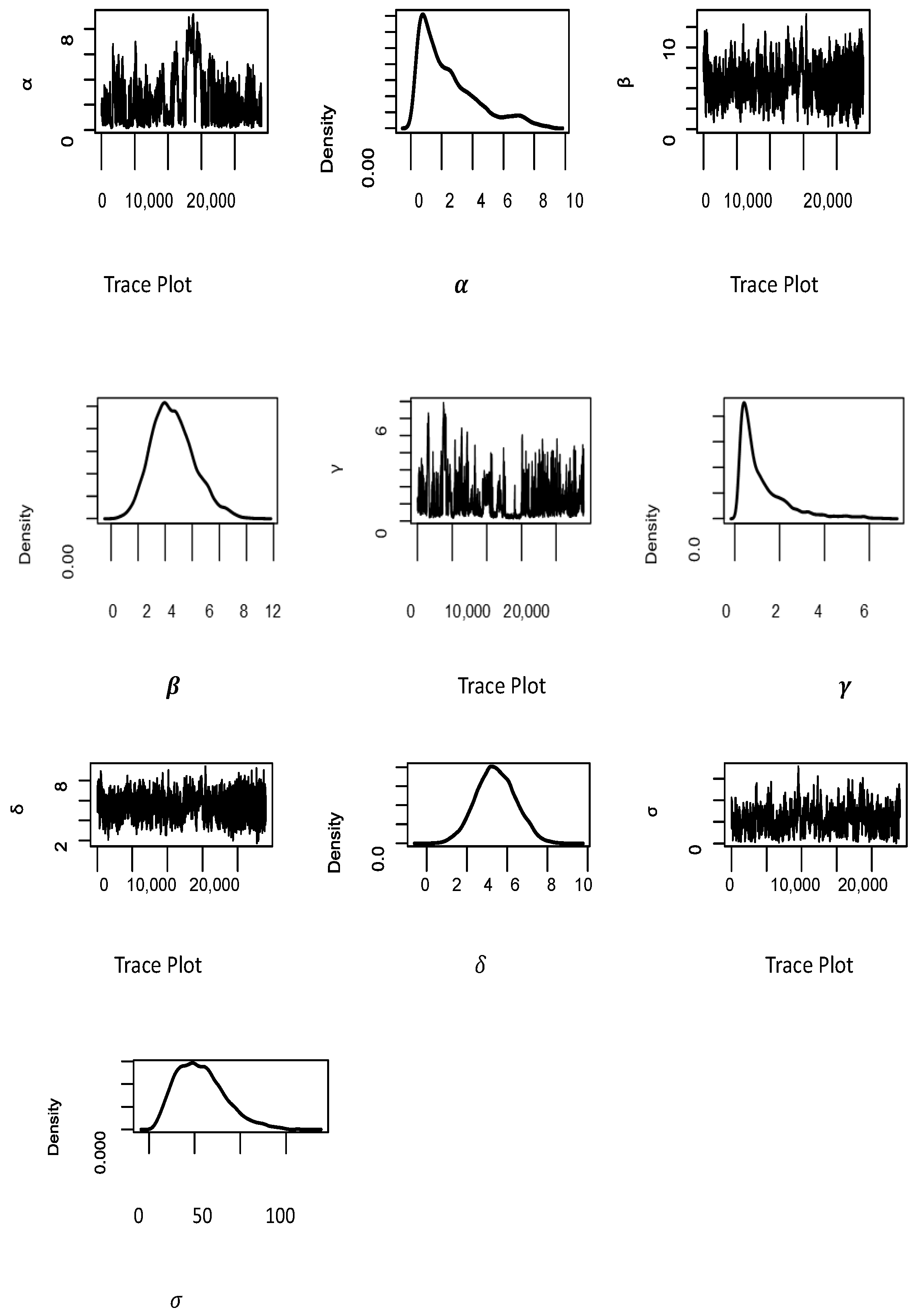
The maximum likelihood estimation and Bayesian analysis of the proposed bivariate model for given data is performed using R packages [50,51], respectively. The results of MLEs are given in Table 1 and contour plot in Figure 6, which shows that our model fits the data well. For Bayesian analysis, defuse inverse Gamma distribution is used as prior and metropolis hasting algorithm is used and the results are given in Table 2. The Metropolis acceptance rate is 0.32139, which meets the standard value described in the literature. We use thinning interval 5, which helps to reduce correlation in the samples. The burns-in is planned to give the Markov Chain time to arrive at its balance dispersion. We have used burn-in of 20,000 and a total iteration of 139,996 run with a sample of size 24,000 per chain. Figure 7 shows that the parameters seem to be rather stable.
7. Conclusions
In this research, a new Bivariate Exponential Wiebull Inverse Lomax distribution (BEWIL) is proposed by compounding two independent asymmetric univariate nested distributions to model the availability of the system. The aging properties of BEWIL are also derived. The real-life data are exposed to show the efficacy of the new proposed model. To support the model efficacy, graphical presentations are also reported. The parameters of the proposed model are estimated by both the classical (MLE) and Bayesian approaches. The newly proposed bivariate distribution BEWIL appears to model system availability well. Our proposed model BEWIL is suitable for modeling the survival of systems which depend on two independent components, which makes it flexible to implement in different fields of research like medical, environment, agriculture and others. Although the proposed model is rather flexible, it has limitation that cannot be implemented to a scenario wherein the components are dependent. The researcher can extended this work to model the phenomena with dependent structures. The researchers can also derive test statistic to test the hypothesis. The suggested model addresses the problem of availability of a system in the presence of independent components, and can be implemented in several fields.
Author Contributions
Conceptualization: M.F., A.G. and H.M.A. Methodology: M.F., H.M.A. and S.K.K. Software: M.F., H.M.A. and A.G. Validation: M.F., H.M.A. and S.K.K. Formal analysis: M.F., A.G. and H.M.A. Investigation: H.M.A. and S.K.K. Resources: H.M.A. Data curation: S.K.K. Writing—original draft preparation: M.F. and A.G. writing—review and editing: H.M.A. and S.K.K. Project administration: A.G. Funding acquisition: H.M.A. All authors have read and agreed to the published version of the manuscript.
Funding
Princess Nourah bint Abdulrahman University Researchers Supporting Project number (PNURSP2023R 299), Princess Nourah bint Abdulrahman University, Riyadh, Saudi Arabia.
Data Availability Statement
The relevant data is available in the manuscript.
Conflicts of Interest
The authors declare that they have no conflict of interest.
References
- Lancaster, H. The structure of bivariate distributions. Ann. Math. Stat. 1958, 29, 719–736. [Google Scholar] [CrossRef]
- Gumbel, E.J. Bivariate exponential distributions. J. Am. Stat. Assoc. 1960, 55, 698–707. [Google Scholar] [CrossRef]
- Freund, J.E. A bivariate extension of the exponential distribution. J. Am. Stat. Assoc. 1961, 56, 971–977. [Google Scholar] [CrossRef]
- Marshall, A.W.; Olkin, I. A multivariate exponential distribution. J. Am. Stat. Assoc. 1967, 62, 30–44. [Google Scholar] [CrossRef]
- Block, H.W.; Basu, A. A continuous, bivariate exponential extension. J. Am. Stat. Assoc. 1974, 69, 1031–1037. [Google Scholar]
- Ali, M.M.; Mikhail, N.; Haq, M.S. A class of bivariate distributions including the bivariate logistic. J. Multivar. Anal. 1978, 8, 405–412. [Google Scholar] [CrossRef]
- Holland, P.W.; Wang, Y.J. Dependence function for continuous bivariate densities. Commun. Stat.-Theory Methods 1987, 16, 863–876. [Google Scholar] [CrossRef]
- Arnold, B.C.; Ng, H.K.T. Flexible bivariate beta distributions. J. Multivar. Anal. 2011, 102, 1194–1202. [Google Scholar] [CrossRef]
- Lee, H.; Cha, J.H. On construction of general classes of bivariate distributions. J. Multivar. Anal. 2014, 127, 151–159. [Google Scholar] [CrossRef]
- Downton, F. Bivariate exponential distributions in reliability theory. J. R. Stat. Soc. Ser. B (Methodol.) 1970, 32, 408–417. [Google Scholar] [CrossRef]
- Bemis, B.M. Some Statistical Inferences for the Bivariate Exponential Distribution. Ph.D. Thesis, University of Missouri, Rolla, MO, USA, 1971. [Google Scholar]
- Hougaard, P. Modelling multivariate survival. Scand. J. Stat. 1987, 14, 291–304. [Google Scholar]
- Wang, C. Analysis of a New Bivariate Distribution in Reliability Theory. Doctor’s Dissertation, The University of Arizona, Tucson, AZ, USA, 2000. [Google Scholar]
- Filus, J.; Filus, L. On two new methods for constructing multivariate probability distributions with system reliability motivations. In Proceedings of the Applied Stochastic Models and Data Analysis Conference, ‘ASMDA, Brest, France, 17–20 May 2005; pp. 17–20. [Google Scholar]
- Sarper, H. Reliability analysis of descent systems of planetary vehicles using bivariate exponential distribution. In Proceedings of the Annual Reliability and Maintainability Symposium, Alexandria, VA, USA, 24–27 January 2005; pp. 165–169. [Google Scholar]
- Nadarajah, S.; Kotz, S. Reliability for a bivariate gamma distribution. Stochastics Qual. Control 2005, 20, 111–119. [Google Scholar] [CrossRef]
- Nadarajah, S.; Kotz, S. Reliability for some bivariate exponential distributions. Math. Probl. Eng. 2006, 2006, 041652. [Google Scholar] [CrossRef]
- Pulcini, G. A bivariate distribution for the reliability analysis of failure data in presence of a forewarning or primer event. Commun. Stat.-Theory Methods 2006, 35, 2107–2126. [Google Scholar] [CrossRef]
- Nadarajah, S.; Kotz, S. The beta exponential distribution. Reliab. Eng. Syst. Saf. 2006, 91, 689–697. [Google Scholar] [CrossRef]
- Gupta, R.C. Reliability studies of bivariate distributions with exponential conditionals. Math. Comput. Model. 2008, 47, 1009–1018. [Google Scholar] [CrossRef]
- Ahsanullah, M.; Shahbaz, S.; Shahbaz, M.Q.; Mohsin, M. Concomitants of upper record statistics for bivariate pseudo–weibull distribution. Appl. Appl. Math. 2010, 5, 1379–1388. [Google Scholar]
- Yunus, R.M.; Khan, S. The bivariate noncentral chi-square distribution—A compound distribution approach. Appl. Math. Comput. 2011, 217, 6237–6247. [Google Scholar] [CrossRef]
- O’Connor, A.N. Probability Distributions Used in Reliability Engineering; Center for Risk and Reliability: College Park, MD, USA, 2011. [Google Scholar]
- Gupta, P.L.; Gupta, R.C. Some properties of the bivariate lognormal distribution for reliability applications. Appl. Stoch. Model. Bus. Ind. 2012, 28, 598–606. [Google Scholar] [CrossRef]
- Tang, X.-S.; Li, D.-Q.; Zhou, C.-B.; Zhang, L.-M. Bivariate distribution models using copulas for reliability analysis. Proc. Inst. Mech. Eng. Part O J. Risk Reliab. 2013, 227, 499–512. [Google Scholar] [CrossRef]
- Tang, X.-S.; Li, D.-Q.; Zhou, C.-B.; Phoon, K.-K.; Zhang, L.-M. Impact of copulas for modeling bivariate distributions on system reliability. Struct. Saf. 2013, 44, 80–90. [Google Scholar] [CrossRef]
- Navarro, J.; Sarabia, J.M. Reliability properties of bivariate conditional proportional hazard rate models. J. Multivar. Anal. 2013, 113, 116–127. [Google Scholar] [CrossRef]
- Verrill, S.P.; Evans, J.W.; Kretschmann, D.E.; Hatfield, C.A. Reliability implications in wood systems of a bivariate gaussian–weibull distribution and the associated univariate pseudo-truncated weibull. J. Test. Eval. 2014, 42, 412–419. [Google Scholar] [CrossRef]
- Gupta, R.C. Reliability studies of bivariate birnbaum-saunders distribution. Probab. Eng. Inf. Sci. 2015, 29, 265. [Google Scholar] [CrossRef]
- El-Damcese, M.; Mustafa, A.; Eliwa, M. Bivariate exponentaited generalized weibull-gompertz distribution. arXiv 2015, arXiv:1501.02241. [Google Scholar]
- Khan, S.; Pratikno, B.; Ibrahim, A.I.; Yunus, R.M. The correlated bivariate noncentral f distribution and its application. Commun. Stat.-Simul. Comput. 2016, 45, 3491–3507. [Google Scholar] [CrossRef]
- Klein, B.; Meissner, D.; Kobialka, H.-U.; Reggiani, P. Predictive uncertainty estimation of hydrological multi-model ensembles using pair-copula construction. Water 2016, 8, 125. [Google Scholar] [CrossRef]
- Vaidyanathan, V.S.; Sharon Varghese, A. Morgenstern Type Bivariatelindley Distribution. Stat. Optim. Inf. Comput. 2016, 4, 132–146. [Google Scholar] [CrossRef]
- Mercier, S.; Pham, H.H. A bivariate failure time model with random shocks and mixed effects. J. Multivar. Anal. 2017, 153, 33–51. [Google Scholar] [CrossRef]
- Lee, H.; Cha, J.H.; Pulcini, G. Modeling discrete bivariate data with applications to failure and count data. Qual. Reliab. Int. 2017, 33, 1455–1473. [Google Scholar] [CrossRef]
- Ibrahim, M.; Eliwa, M.; Morshedy, M.E. Bivariate exponentiated generalized linear exponential distribution with applications in reliability analysis. arXiv 2017, arXiv:1710.00502. [Google Scholar]
- Yuan, F.; Barabadi, A.; Lu, J. Reliability modelling on two-dimensional life data using bivariate weibull distribution: With case study of truck in mines. Eksploat. Niezawodn. 2017, 19, 650–659. [Google Scholar]
- Tahmasebi, S.; Jafari, A.A.; Ahsanullah, M. Reliability characteristics of bivariate rayleigh distribution and concomitants of its order statistics and record values. Stud. Sci. Math. Hung. 2017, 54, 151–170. [Google Scholar] [CrossRef]
- Temraz, N.S.Y. Availability and Reliability Analysis for Dependent System with Load-Sharing and Degradation Facility. Int. J. Syst. Sci. Appl. Math. 2018, 3, 10–15. [Google Scholar] [CrossRef]
- Hu, Z.; Zhu, Z.; Du, X. Time-dependent system reliability analysis for bivariate responses. ASCE-ASME J. Risk Uncertain. Eng. Syst. 2018, 4, 031002. [Google Scholar] [CrossRef]
- Goharian, E.; Burian, S.J.; Karamouz, M. Using joint probability distribution of reliability and vulnerability to develop a water system performance index. J. Water Resour. Plan. Manag. 2018, 144, 04017081. [Google Scholar] [CrossRef]
- Sarhan, A. The bivariate generalized rayleigh distribution. J. Math. Sci. Model. 2019, 2, 99–111. [Google Scholar] [CrossRef]
- Vineshkumar, B.; Nair, N.U. Bivariate quantile functions and their applications to reliability modelling. Statistica 2019, 79, 3–21. [Google Scholar]
- Yang, Z.; Huang, W.; Dong, S.; Li, H. Mixture bivariate distribution of wind speed and air density for wind energy assessment. Energy Convers. Manag. 2023, 276, 116540. [Google Scholar] [CrossRef]
- Farooq, M.M.; Mohsin, M.; Farman, M.; Akgül, A.; Saleem, M.U. Generalization method of generating the continuous nested distributions. Int. J. Nonlinear Sci. Numer. 2022, 24, 1327–1353. [Google Scholar] [CrossRef]
- Johnson, N.L.; Kotz, S. A vector multivariate hazard rate. J. Multivar. Anal. 1975, 5, 53–66. [Google Scholar] [CrossRef]
- Lemoine, N.P. Moving beyond noninformative priors: Why and how to choose weakly informative priors in bayesian analyses. Oikos 2019, 128, 912–928. [Google Scholar] [CrossRef]
- Demirhan, H.; Kalaylioglu, Z. Joint prior distributions for variance parameters in bayesian analysis of normal hierarchical models. J. Multivar. Anal. 2015, 135, 163–174. [Google Scholar] [CrossRef]
- Hamada, M.S.; Wilson, A.; Reese, C.S.; Martz, H. Bayesian Reliability; Springer: Berlin/Heidelberg, Germany, 2008. [Google Scholar]
- Henningsen, A.; Toomet, O. maxlik: A package for maximum likelihood estimation in R. Comput. Stat. 2011, 26, 443–458. [Google Scholar] [CrossRef]
- Martin, A.D.; Quinn, K.M.; Park, J.H. MCMCpack: Markov chain monte carlo in R. J. Stat. Softw. 2011, 42, 22. [Google Scholar] [CrossRef]
Figure 1.
Contour plot for different parameteric combinations.
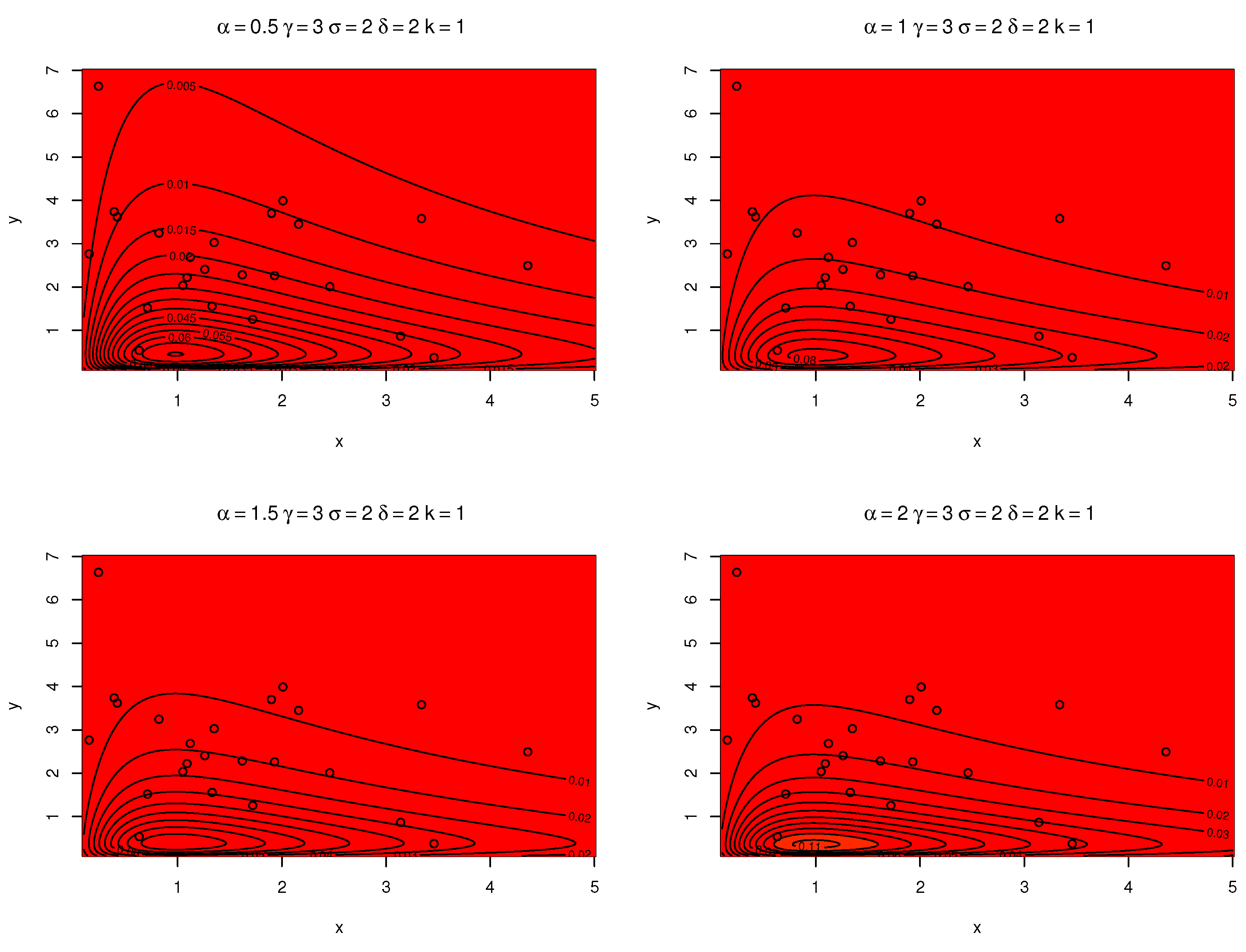
Figure 2.
Contour plot for different parameteric combinations.

Figure 3.
Contour plot for different parameteric combinations.
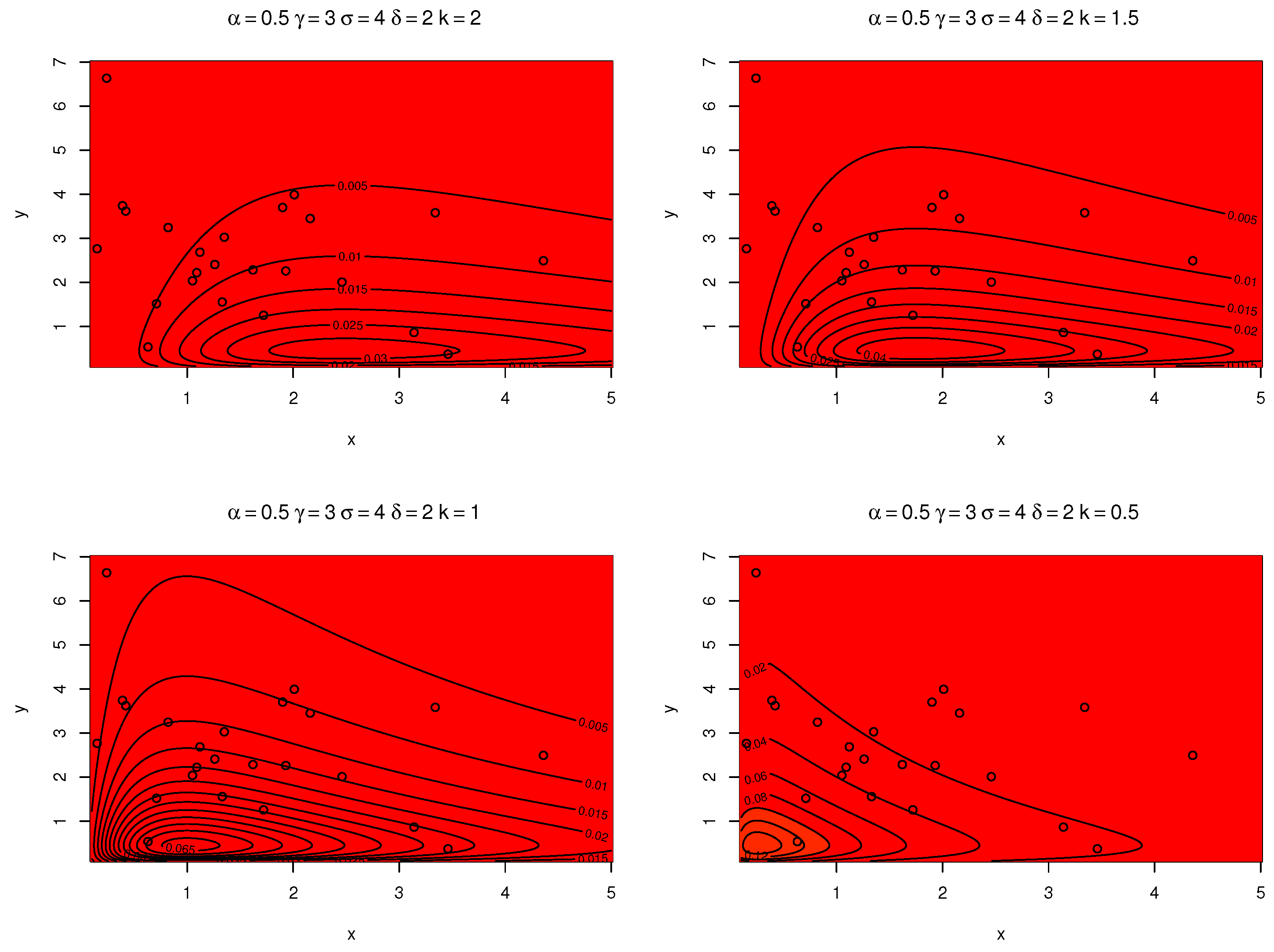
Figure 4.
Contour plot for different parametric combinations.
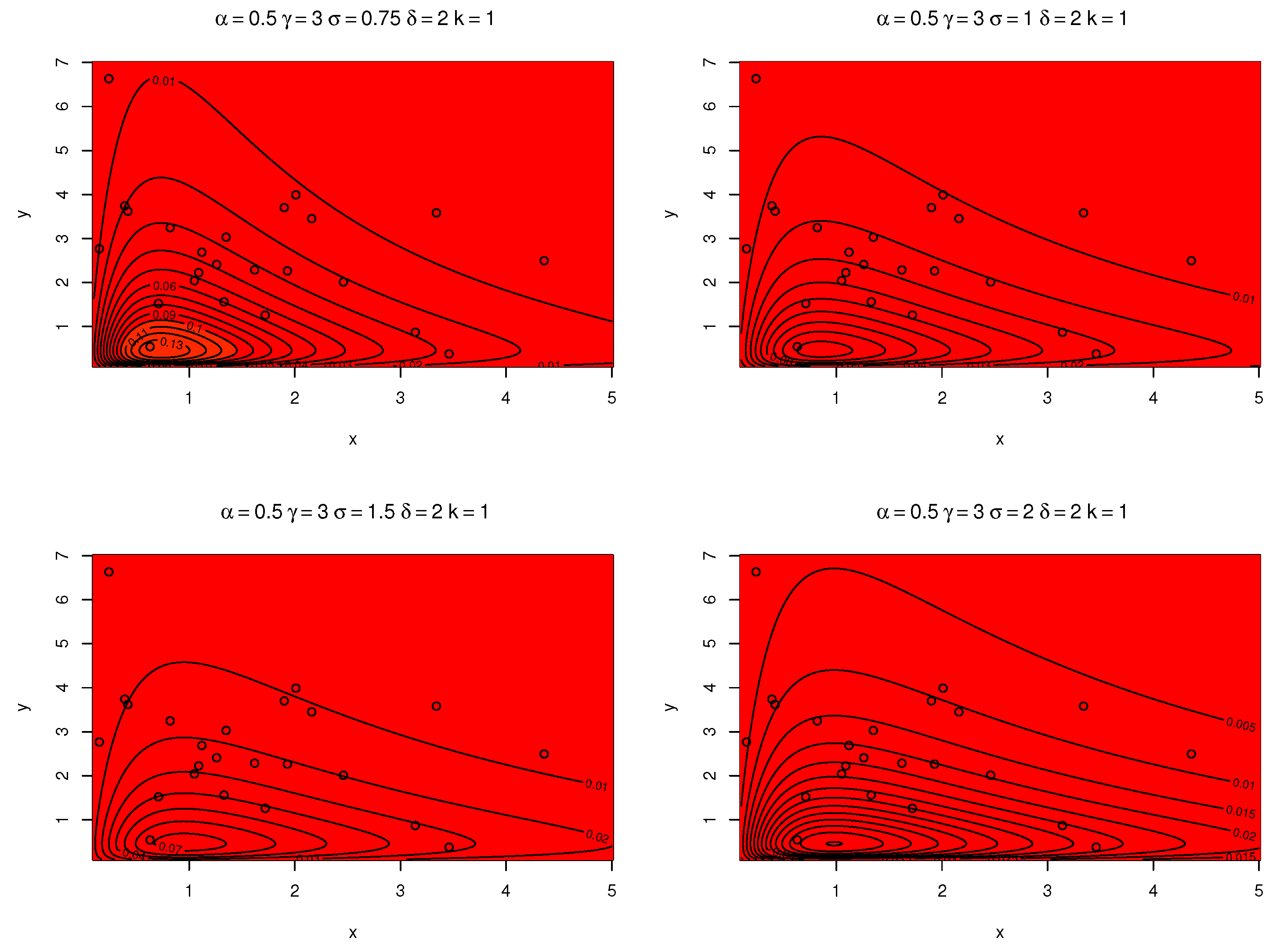
Figure 5.
Distribution of total time of failure and repair.
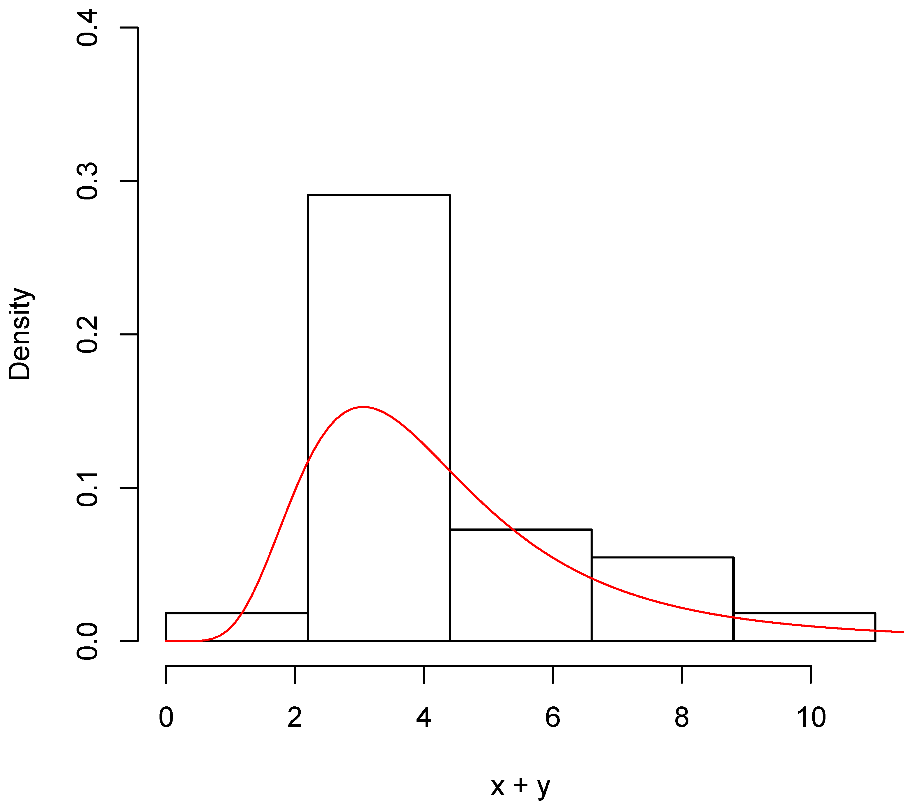
Figure 6.
Contour plot of system availability data using ML estimates.
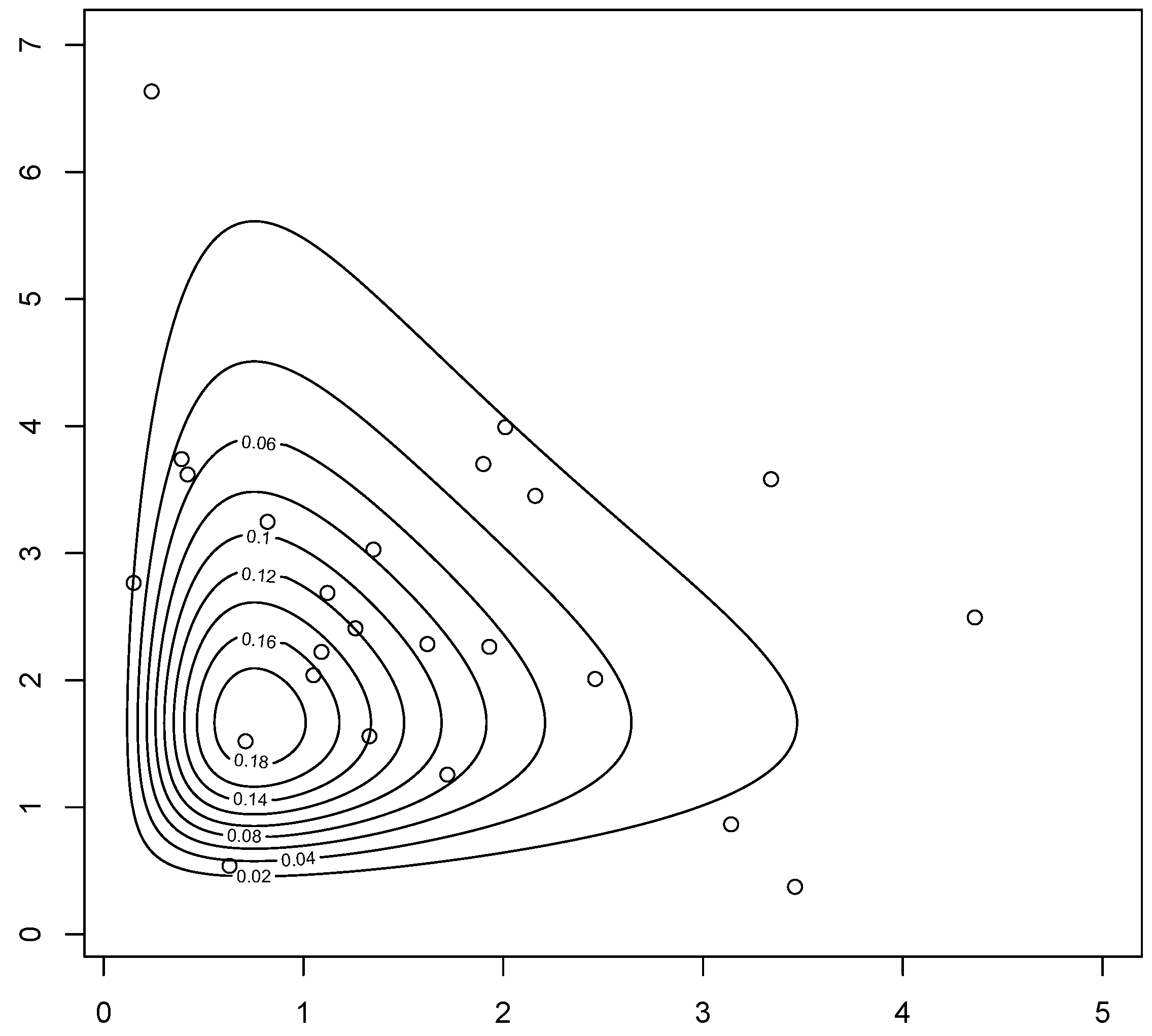
Figure 7.
Shapes of the posterior distributions along with the trace plots of the model parameters for system availability data.
Figure 7.
Shapes of the posterior distributions along with the trace plots of the model parameters for system availability data.

Table 1.
ML estimates of bivariate model for availability data.
| Parameter | Estimate | Std. Error |
|---|---|---|
| 2.2338 | 8.9739 | |
| 7.3106 | 2.8615 | |
| 1.5520 | 6.2469 | |
| 6.5401 | 1.2143 | |
| 0.3471 | 1.4763 | |
| negative log likelihood | −84.95289 |
Table 2.
Summary statistics of the posterior distribution for and .
| Parameters | Mean | Median | S.D. | 25th Percentile | 75th Percentile | 95% CI |
|---|---|---|---|---|---|---|
| 3.1943 | 2.4371 | 2.3911 | 1.5710 | 4.0391 | 0.861–9.971 | |
| 4.5209 | 3.4703 | 1.5316 | 3.4703 | 5.4544 | 1.781–7.795 | |
| 0.7314 | 0.6402 | 0.4271 | 0.3943 | 0.9843 | 0.170–1.753 | |
| 5.3925 | 5.4016 | 0.9523 | 4.7636 | 6.0232 | 3.50–7.24 | |
| 63.9082 | 60.4044 | 30.9696 | 41.6535 | 79.0033 | 19.107–156.206 |
Disclaimer/Publisher’s Note: The statements, opinions and data contained in all publications are solely those of the individual author(s) and contributor(s) and not of MDPI and/or the editor(s). MDPI and/or the editor(s) disclaim responsibility for any injury to people or property resulting from any ideas, methods, instructions or products referred to in the content. |
© 2023 by the authors. Licensee MDPI, Basel, Switzerland. This article is an open access article distributed under the terms and conditions of the Creative Commons Attribution (CC BY) license (https://creativecommons.org/licenses/by/4.0/).
Share and Cite
MDPI and ACS Style
Farooq, M.; Gul, A.; Alshanbari, H.M.; Khosa, S.K. Modeling of System Availability and Bayesian Analysis of Bivariate Distribution. Symmetry 2023, 15, 1698. https://doi.org/10.3390/sym15091698
AMA Style
Farooq M, Gul A, Alshanbari HM, Khosa SK. Modeling of System Availability and Bayesian Analysis of Bivariate Distribution. Symmetry. 2023; 15(9):1698. https://doi.org/10.3390/sym15091698
Chicago/Turabian StyleFarooq, Muhammad, Ahtasham Gul, Huda M. Alshanbari, and Saima K. Khosa. 2023. "Modeling of System Availability and Bayesian Analysis of Bivariate Distribution" Symmetry 15, no. 9: 1698. https://doi.org/10.3390/sym15091698
Note that from the first issue of 2016, this journal uses article numbers instead of page numbers. See further details here.