
Recent Advances in Inflation
by
 , , and
Sergei D. Odintsov
1,2,
Vasilis K. Oikonomou
3,4,*,
Ifigeneia Giannakoudi
5,6,
Fotis P. Fronimos
3 and
Eirini C. Lymperiadou
3,7
1
ICREA, Passeig Luis Companys, 23, 08010 Barcelona, Spain
2
Institute of Space Sciences (ICE, CSIC), C. Can Magrans s/n, 08193 Barcelona, Spain
3
Department of Physics, Aristotle University of Thessaloniki, 54124 Thessaloniki, Greece
4
Laboratory for Theoretical Cosmology, International Center of Gravity and Cosmos, Tomsk State University of Control Systems and Radioelectronics (TUSUR), 634050 Tomsk, Russia
5
University of Waterloo, Waterloo, ON N2L 3G1, Canada
6
Perimeter Institute, Waterloo, ON N2L 2Y5, Canada
7
Department of Physics and Astronomy, University of Bonn, 53127 Bonn, Germany
*
Author to whom correspondence should be addressed.
Symmetry 2023, 15(9), 1701; https://doi.org/10.3390/sym15091701
Submission received: 30 July 2023
/
Revised: 24 August 2023
/
Accepted: 29 August 2023
/
Published: 5 September 2023
(This article belongs to the Special Issue Physics and Symmetry Section: Feature Papers 2023)
Abstract
:We review recent trends in inflationary dynamics in the context of viable modified gravity theories. After providing a general overview of the inflationary paradigm emphasizing on what problems hot Big Bang theory inflation solves, and a somewhat introductory presentation of single-field inflationary theories with minimal and non-minimal couplings, we review how inflation can be realized in terms of several string-motivated models of inflation, which involve Gauss–Bonnet couplings of the scalar field, higher-order derivatives of the scalar field, and some subclasses of viable Horndeski theories. We also present and analyze inflation in the context of Chern–Simons theories of gravity, including various subcases and generalizations of string-corrected modified gravities, which also contain Chern–Simons correction terms, with the scalar field being identified with the invisible axion, which is the most viable to date dark matter candidate. We also provide a detailed account of vacuum gravity inflation, and also inflation in and kinetic-corrected theories of gravity. At the end of the review, we discuss the technique for calculating the overall effect of modified gravity on the waveform of the standard general relativistic gravitational wave form.
1. Introduction
Physicists of the current era are lucky to live in the era of precision cosmology, in which a plethora of observational data are available. Without exaggeration, nearly every 3 years, a great discovery takes place. It started in 2012 with the Higgs discovery at the LHC [1], followed by the first direct observation of gravitational waves in 2015 [2], followed by the one in a million kilonova event in 2017, nowadays known as GW170817 [3]. After that, in 2020, the NANOGrav collaboration reported on the discovery of something that could be either a pulsar red noise, or a gravitational wave [4]. The latter was verified in 2023, the year in which the NANOGrav reported the first detection of a stochastic gravitational wave background, verified by Hellings–Downs correlations, so the signal is clearly a gravitational wave of cosmological or astrophysical origin [5]. The chorus of observations will be further augmented by future experiments, like the stage 4 Cosmic Microwave Background (CMB) experiments [6,7], expected to commence operations in 2027, and future gravitational wave experiments [8,9,10,11,12,13,14,15,16], like LISA and the Einstein Telescope, which will commence their operation in 2035. All these new experiments will shed light on fundamental problems in cosmology and astrophysics. The most important of all, they will probe the primordial tensor modes in our universe and give a definitive answer on the question of whether inflation ever occurred. The inflationary scenario [17,18,19] is one of the most viable theoretical proposals for the early time era of our universe. This is because inflation as a proposal solves all the basic problems of the standard hot Big Bang model, and in addition it serves as a mechanism for generating matter structures at large scales in our universe. The primordial quantum fluctuations generated during the inflationary era act as attractors on which baryons and cold dark matter are accumulated, so the large-scale structure at the large redshift up to may be explained by a nearly scale invariant power spectrum of primordial scalar perturbations. Thus, from a theoretical point of view, the inflationary scenario is the most appealing and vital for the viable description of the primordial evolution of the universe, and for explaining the large-scale structure of the universe. In principle, many theoretical frameworks may generate an accelerating era primordially; for a main stream of articles and reviews, see [17,18,19,20,21,22,23,24,25,26,27,28,29,30,31,32,33,34,35,36,37,38,39,40,41,42,43,44,45,46,47,48,49,50,51,52,53,54,55,56,57,58,59,60,61,62,63,64,65,66,67,68,69,70,71,72,73,74,75,76,77,78,79,80,81,82,83,84,85,86,87,88,89,90,91,92,93,94,94]. Traditionally, the inflationary scenario was firstly considered in terms of some false vacuum decay of a scalar field [17], but it was then realized that a slow-rolling canonical scalar field may appropriately describe the inflationary era [18]. Usually inflation is formalized by the use of a canonical minimally coupled scalar field or by a non-minimally coupled scalar field; however, there are many shortcomings of the scalar field description of inflation that make an alternative description rather compelling. The most important shortcoming is that the single scalar field description relies on a scalar field, which must couple to all the Standard Model particles in order to reheat the universe. Thus, there are too many unknown arbitrary couplings that must be explained, and also the inflaton itself must be identified or experimentally verified. The only fundamental scalar field that has ever been observed is the Higgs particle, so inflationary scenarios that use the Higgs particle as the inflaton are well motivated [95]. There exist, however, models that assume that the axion is the inflaton, with the axion also being a dark matter candidate. However, this could be deemed problematic, since if the axion is the inflaton, it must couple to Standard Model particles in order to reheat the universe. This is a rather unwanted situation since in most contexts, the axion is a non-thermal relic. Regardless of the theoretical shortcomings, the scalar field inflationary models are the most common and frequently used descriptions of inflation. An alternative to scalar field inflationary models comes from modifications of Einstein–Hilbert gravity, which contain higher-order curvature corrections. There are many modified gravity models; for some important reviews in the field, see refs. [96,97,98,99,100,101]. The most important and more common models of modified gravity use gravity, with R being the Ricci scalar; see refs. [96,97,98,99,100,101]. These models are simple and mainstream models and can also have an Einstein frame counterpart theory, which is a minimally coupled scalar field. One important feature of this gravity framework is that it is possible to achieve a unified description of inflation with the dark energy era; see the pioneer work on this [102] and several works thereafter [43,103,104,105,106,107,108,109,110,111]. Since the GW170817 event, it has been made clear that gravitational waves propagate with the velocity of light. While some may argue that this is a late-time result, and therefore, a varying gravitational wave velocity could in principle manifest primordially, it is reasonable to believe that it remains constant throughout the evolution of the universe. While many models that predict a propagation velocity that deviates from the speed of light are excluded, the gravity is not excluded since it predicts . Apart from gravity inflation, modified Gauss–Bonnet theories of gravity are also well studied in the literature of the form [112,113,114,115,116] or [117], where G is the Gauss–Bonnet scalar. The theories are plagued with ghost instabilities and degrees of freedom; thus, they are less frequently used and are less appealing. In addition, quite popular theories are the Einstein–Gauss–Bonnet theories of gravity [113,114,118,119,120,121,122,123,124,125,126,127,128,129,130,131,132,133,134,135,136,137,138,139,140,141,142,143,144,145,146,147,148,149,150,151,152,153,154,155,156,157,158,159,160], but these theories are plagued with a non-trivial gravitational wave speed, which is distinct from the speed of light in vacuum. These theories were severely constrained after the GW170817 event since the latter indicated that the electromagnetic signal arrived almost simultaneously with the gravitational waves. However, a theoretical solution for this problem was given recently in refs. [158,159], in which case the theory resulted in a constraint between the scalar field potential and the Gauss–Bonnet coupling function. In addition, models of gravity are also used to produce inflation, and also Chern–Simons models of inflation are also used. In addition, several models can also describe the inflationary era, where T is the trace of the energy momentum tensor; see the reviews [96,97]. Also, two scalar field models are used for inflation, see [83].
The recent NANOGrav observation of the stochastic signal of gravitational waves, if interpreted as a cosmological signal, indicates that the inflationary era must have had a blue tilt in its tensor spectral index, a fact that severely constrains the inflationary models that can reproduce such a signal. This can be achieved by Einstein–Gauss–Bonnet models, at the cost of having a low-reheating temperature, see for example [55,161], while single canonical scalar field models, under the slow-roll assumption, without gravity modifications cannot explain the 2023 NANOGrav signal. Of course, further measurements are required to decipher the origin of the stochastic signal, whether it is primarily astrophysical or cosmological; however a primordial interpretation can significantly constrain the inflationary models, or even exclude these. Note that, currently, the astrophysical interpretation is challenged in a three-fold way: firstly, the final parsec problem is not solved even theoretically; secondly, no large anisotropies are detected in the observed signal; and thirdly, no single binary of supermassive black holes is observed. Thus, the current epoch puts severe constraints on theoretical frameworks, which must explain the observations that come out in an incredible speedy way nowadays. Thus, to rise to the challenge, the modern theoretical physicist must master the techniques of inflationary cosmology and know how to judge whether a theoretical model is viable or not. In this review, we aim to provide a timely text which contains all the recent trends and techniques on inflationary dynamics but also discussing the standard problems of Big Bang cosmology and why inflation itself describes successfully in a theoretical way the primordial era of our universe. We analyze inflationary dynamics in a quantitative way for single scalar field inflation, both minimally and non-minimally coupled, and for most mainstream modified gravity theories, including those for which the tensor spectral index can be blue tilted, a necessary ingredient in order for the models to be compatible with the NANOGrav stochastic gravitational wave observation if the cosmological description is responsible for the signal of course. Our analysis is limited to providing the necessary tools in order for someone to be able to produce viable inflationary cosmologies, compatible with the most recent (2018) Planck constraints on inflation [162].
The scalar and the tensor power spectrum can be written in terms of a certain set of dimensionless parameters, which are known as “slow-roll” parameters. When these are smaller than unity, a perturbation expansion can be performed on the scalar and tensor power spectrum, and the observable quantities which quantify the inflationary era can be expressed in terms of the slow-roll parameters. Regarding the observable quantities of inflation, we focus on the most important ones, which are the spectral index of the scalar primordial curvature perturbations, the tensor spectral index of the primordial tensor perturbations and the tensor-to-scalar ratio. Depending on the theoretical framework, the number and the complexity of the slow-roll parameters vary, so we emphasize the calculation of the slow-roll parameters for various mainstream theoretical frameworks, and we express the observational quantities of inflation in terms of the slow-roll indices needed for each theory. We also provide relations in closed form for all the observational quantities and the corresponding slow-roll indices so that the reader is able to reproduce the results quoted in each case. In the end of the review, we provide a concrete self-contained section on the evolution of tensor perturbations in the context of modified gravity, and we quantify the effect of modified gravity in terms of a single parameter. Then, we analyze how the general relativistic waveform of the tensor perturbation may acquire a non-trivial multiplicative factor, which contains the overall modified gravity effect from the present day back to the redshift corresponding to the mode that reentered the Hubble horizon back in our universe’s past.
We need to note that the inflationary scenario is a theoretical necessity in order to alleviate the problems of standard hot Big Bang cosmology. Even if we have no direct sign that inflation ever occurred, the observations “cry for inflation” since it is the only consistent scenario that can be compatible with the observational necessity of having a nearly scale invariant power spectrum of primordial perturbations, and it is the only consistent answer to the question how the large-scale matter structure was generated in the first place. Inflation and dark matter are theoretical predictions that still wait to be revealed observationally and experimentally. We may still be far away from discovering those theoretical predictions, and even if we did not find them yet, it is almost certain in the minds of theorists that both play an important role in the evolution of the universe. The situation here is the same as in the discovery of the Higgs, where every theorist believed that the elusive spinless particle gives mass to the Standard Model particles, but it was never observed until 2012. We all knew it was there and only the proof of its existence remained to be found. And we knew because the Higgs particle and the electroweak symmetry breaking was the only theoretical mechanism that could yield a mass to the Standard Model particles. The same applies with the inflationary paradigm. It must be the underlying mechanism responsible for the CMB anisotropies and the reason that large scale matter structure exists, and we need to find a proof for its existence. Inflation is not the only paradigm of which its predictions can alleviate some of the cosmological issues, as there are other scenarios as well. A rather known paradigm revolves around bouncing cosmology, such as the ekpyrotic scenario. The latter is quite interesting since it can generate a positive tensor spectral index and thus is capable of explaining the NanoGrav results discussed before. In this review, we focus strictly on the inflation paradigm. The road might be long and thorny till we unveil inflation, or the proof might be right at the corner of our “local time frame of inertia”. Nobody knows, and that is the magic of nature.
This review is organized as follows: In Section 2, we provide an overview of the inflationary paradigm. We point out the shortcomings of the standard hot Big Bang scenario, and we explain how the inflationary paradigm theoretically solves these problems. We emphasize how important the inflationary paradigm is theoretically, and why it eventually could be the correct description of nature since it is the only scenario which provides a nearly scale invariant power spectrum of primordial scalar curvature fluctuations, which are necessary in order to explain the large-scale structure of our universe as a whole. In Section 3, we analyze in detail how the inflationary era may be generated by a single scalar field theory with minimal and non-minimal couplings. We calculate the necessary slow-roll indices, and we provide and prove in detail several well-known formulas regarding single scalar field inflation. In Section 4, we provide a brief account of the swampland criteria, while in Section 5, we discuss in brief the constant-roll evolution as an alternative to the standard slow-roll evolution. In Section 6, we study and analyze several string motivated models of inflation, which also involve Gauss–Bonnet couplings of the scalar field, higher-order derivatives of the scalar field, and some subclasses of viable Horndeski theories. In Section 7, we present and analyze inflation in the context of Chern–Simons theories of gravity, presenting various subcases and generalizations of string-corrected modified gravities, which also contain Chern–Simons correction terms, with the scalar field being identified with the invisible axion, which is the most viable dark matter candidate to date. Section 8 is devoted to inflation in its most general form in Section 8.1, and generalized theories of gravity, in the form of Section 8.2 and Section 8.3, while Section 9 focuses on kinetic-corrected theories of gravity. Finally, in Section 10, we provide a concrete overview of the evolution equations for the tensor perturbations in the context of modified gravity and we review how to calculate the overall effect of modified gravity on the general relativistic gravitational wave waveform. Finally, Section 11 follows at the end of the review.
2. Brief Overview of Inflation
In the early period of the 1970s, physicists started to realize some problematic elements of the conventional Big Bang model, and thus the first aspects of inflationary cosmology started to be formulated. Different characteristics of the mechanics for inflation were discovered, and the first somewhat realistic model, in which the early universe went through an inflationary de Sitter era, was proposed by Starobinsky [19]. Also an equally important point in the historical development of inflation was the model proposed by Guth [17], in which the inflationary era was a period when the universe exponentially expanded in a super-cooled false vacuum state (a metastable state with no particles or fields but large vacuum energy density). However, due to the possible outcomes of this model, it was recognized that it is not realistic and viable even with improvements in order to explain several shortcomings of Big Bang cosmology. The solution was given by Linde [18], who proposed the “new inflationary theory” [18], in which inflation can start either in a false vacuum or at the top of an effective potential in an unstable state and then the inflationary field slowly rolls down to the minimum of that effective potential. Various models for inflation have been constructed ever since. The main fundamental idea for all of them is the following:
Inflation is an era of an abrupt accelerated expansion that took place in a very early period after the beginning of the Universe.
Some follow a canonical approach using scalar fields, and others use a description based on modified gravity for inflation, with the most interesting and promising ones being the -gravity models. Descriptions for a lot of these cases are going to be presented in this text; however, we start by presenting the key problematic elements of the Big Bang model that were the reason for introducing inflation as the optimal theoretical description of our universe’s primordial era.
2.1. The Shortcomings of the Hot Big Bang Cosmology
The standard Big Bang (SBB) cosmology paradigm is a very successful model since there are various successful observations about the properties of cosmic objects based on the SBB theory. Also, along with the study of the cosmic microwave background (CMB), SBB guided us to our first understanding of various cosmological phenomena as well as enabling us to gain an understanding of how the universe evolved in the very early epochs of its existence all the way up to the universe’s late time large-scale form. However, even though the SBB scenario found success and was highly embraced, one cannot ignore that some of its fundamental features can be problematic.
In the SBB, the early universe is adiabatically expanded and radiation-dominated. The model depends on the assumption of homogeneity and isotropy on large scales (cosmological principle), which lead to the ability to use the Friedmann–Robertson–Walker (FRW) metric for the spacetime of the universe, given by the following form:
where is the scale factor that is associated with the spatial part of the metric and its evolution in time. Depending on the value of constant K, we have three different cases. For , the space described by this metric is flat (flat universe); for , it is a closed universe that could be described with a sphere; and for , the universe is open, with the spatial part of the spacetime being some hyperbolic hypersurface, like a saddle.
In (1), the coordinates used are called the comoving coordinates, meaning that as the universe and thus space itself expands, the coordinates and are not affected by this expansion. The expansion of the universe is encapsulated in the scale factor , and the cosmic objects without peculiar motion have fixed coordinates. To obtain a form of the metric with the physical distance, the scalar factor is multiplied by r, . The metric (1) can be rewritten using a coordinate transformation as [34]
where,
Assuming the FRW metric and (in natural units for example), the evolution of the universe is mainly described by the form of the scalar factor and by transforming the form of the metric with respect to the conformal time , we have
where,
So by using this metric and these coordinates, the structure of the spacetime is more easily visualized. Specifically, in an isotropic universe, the geodesics of propagating light are null . Thus, the radial null geodesics for propagating light in an isotropic, homogeneous universe in the conformal time frame are
which correspond to straight lines at angles of in the (conformal spacetime) plane (see Figure 1).
At this point, two very important quantities must now be introduced. The Hubble parameter H expresses the rate of expansion of the universe and has units of inverse time (or mass units in natural units). It is defined as
where . The Hubble parameter is positive for an expanding universe and negative for a collapsing one. The other important quantity is the e-foldings (or e-folds) number defined as
which represents the number of Hubble times between two epochs with scale factors and . The Hubble time is , which represents the time period that it takes for the universe to expand substantially. The e-folds number can also be given as . In the context of most inflationary cosmologies, the range of the e-folds number for a successful inflationary model that can effectively solve the flatness and horizon problems, which are going to be explained later, is . The previous estimations are based on single scalar field inflationary models, yet the e-folds number is model-dependent and for some specific inflationary models, it is possible that e-folds, a feature that mainly depends on the total equation of the state parameter of the universe at the end of the inflationary era [163]. In other models, e-folds, with having no upper bound that is specifically correlated with the idea of “eternal” inflation [164].
In general, any physical system and its behavior can be described, in the context of the fundamental laws of physics, with the action
where L is the Lagrangian of the system, with an allowed explicit dependence on t [165]. The system follows the path which corresponds to an extremum of the action, which is found by setting the variation of the action equal to zero, ,
and hence, the least action principle leads to the Euler–Lagrange equations of motion for the system
Now, accordingly in the context of field theory, a universe as a physical system can be described by the scalar field action with generic coordinates,
where g is the determinant of a metric and is the Lagrangian density that has dimensions of in natural units, is Lorentz invariant and related to the Lagrangian of the fields by . The equations of motion and basically the evolution of the field can be determined by the same variation principle for the action with respect to the field , and they are called the field equations. Relating to the Lagrangian density , the energy–momentum tensor is defined as
and it is conserved with
Equation (13) can be thought as expressing two continuity equations:
where (14) corresponds to the energy continuity equation and (15) corresponds to the momentum continuity equation in curved spacetime, also known as the Euler equation as well.
On another note, related to the Hubble rate H, by inserting (2) into the Einstein equations, we can derive the following two equations also known as the Friedmann equations:
where , G is the gravitational constant, is the reduced Planck mass, and c the speed of light. When (16) and (17) are combined, they give rise to the continuity equation, or the energy conservation equation:
By defining the equation-of-state parameter ,
and integrating (18), we obtain
which describes how the energy density decays for a specific epoch. So (20), along with the Friedmann Equation (16), leads to the following expression:
which indicates how the scale factor evolves with time [34]. The value of the equation-of-state parameter depends on what perfect fluid energy density dominates the scale factor of the flat universe. Possible values of could be for non-relativistic non-baryonic matter, for vacuum energy (for a cosmological constant), for radiation or relativistic matter, and for stiff matter. Stiff matter is a type of matter that is described by a constant equation-of-state parameter that is identical to unity. This is the maximally allowed value for the equation-of-state parameter since causality demands that has to be strictly less or at the very least equal to 1, while no lower bound appears. In addition, stiff matter describes the strongest type of deceleration in the universe. In the literature, stiff matter has been studied explicitly and in a few cases, it was shown that dark matter may be possible to behave as such. For negative values , the equation-of-state parameter relates to the presence of a dark fluid. For a quintessence and quintessential evolution of the universe, and . The case relates to the existence of hypothetical phantom dark energy, and it can lead to a Big Rip singularity. Data from Planck + WP, SNLS and BAO suggest the limits (95% C.L.) [166]. While the equation-of-state parameter can be taken as a constant, it can also be a function of redshift or time. It is also possible to have significant contributions from various kinds of matter to the total energy density and pressure p; thus, they can be given by the sum of all the individual components as
For each of the components, there is also the ratio of the observed energy density to the critical density for the present time :
where is the density required to make the expansion of the universe slow down, stop and reverse, meaning the existence of a closed universe. Additionally, for the curvature contribution at ,
and using (16), and setting the scalar factor as ,
Therefore, (25) for the present time leads to
Generally as a function of the cosmic time t, the curvature parameter is
and by assuming the simplest case of the expansion being dominated by a form of matter with an equation-of-state parameter and with the scale factor given by and also by taking the first derivative with respect to time, we obtain the following equation:
From (28), it is deduced that the value is an equilibrium point and an unstable one, more specifically. This indicates that if the strong energy condition is satisfied, when deviates a bit from that unstable equilibrium point, for with , the parameter keeps growing and with , keeps decreasing away from zero. From experimental data and observations of large-scale structures and the CMB, it is concluded that (95% C.L.). This means that the presently observed universe is very flat, and therefore it used to be even flatter in the past, with the value of parameter reaching exceptionally small values, . This could be the case if we assumed that precisely for the universe in its very early initial state. However, it seems quite peculiar to have such a precise value of K with no explanation as to why this would be the case.
And this is where the first signs of how some characteristics of the SBB could be problematic and that a new approach is needed appear. The conventional SBB model describes the universe as very homogeneous, isotropic and flat, which are features that do not emerge from a fundamental mechanism that explain how the universe came to be or evolved in that fine-tuned way but only from the initial assumptions of the construction of the model. Apart from the flatness problem, there exist several other shortcomings of the SBB model, and inflation provides concrete theoretical explanations for these problems [17,23]. They are presented one by one in the following subsections.
2.1.1. The Horizon Problem
Before continuing, we will provide definitions of some quantities which are important for better understanding the concepts described here. In (7), the Hubble parameter is defined. There are also the quantities of the Hubble distance, or horizon, given as and the particle horizon , which is the distance that light could have traveled since the beginning when and regions separated by distance more that the particle horizon are “causally disconnected”, meaning they can never communicate with each other. The particle horizon is also called the comoving horizon and is given by the following relation:
where is the comoving Hubble radius and if some regions are separated by a distance greater than the coming Hubble radius, they cannot communicate with each other at that time. By this definition, for a universe dominated with a fluid with an equation-of-state parameter w, the Hubble radius is
So by the conventional SBB, where , the Hubble radius grows monotonically and the comoving horizon increases with time. This means that comoving regions that are entering the horizon in the present time, and thus becoming causally connected now, used to be outside of the limits of the horizon and therefore causally disconnected in the past and especially in the primordial era of the universe. Consequently, the high homogeneity and thermal equilibrium of far distant regions of the universe observed in the CMB that were supposed to be causally disconnected in the early times is quite problematic. This is also sometimes mentioned as the horizon problem. So if homogeneity is not assumed as an initial feature, there must be some mechanism that made the universe evolve that way. However, the SBB model cannot provide an explanation as to how the universe could be that homogeneous without fine-tuning the initial conditions.
Inflation solves this problem by introducing a period with a decreasing comoving Hubble radius . The exponential growth in the scale factor a during inflation and the relatively constant H allows the Hubble radius to be decreasing while inflation is happening. So in the very early period, the comoving Hubble radius was much larger than the comoving horizon and all the scale regions of the universe (relevant to cosmological observation) used to be small enough to be inside the Hubble radius, and thus they were in fact causally connected. Then, during inflation, the radius started to decrease, becoming smaller than the horizon while the volume of the horizon itself expanded. After inflation ended, the Hubble radius started increasing its size again and in consequence, at the present time, the horizon is larger than the Hubble radius, and regions that were causally connected now seem to be causally disconnected; see Figure 2. According to this mechanism, different regions of the universe, which used to be closer together and inside the horizon in the early epoch, were able to communicate, and become homogeneous with respect to each other, and they established thermal equilibrium. When the Hubble radius decreased and the universe rapidly expanded, they became causally disconnected as we observe them to be today.
2.1.2. The Flatness Problem
We briefly discussed the flatness problem, and now we shall further elaborate on this. The second issue that arises is the flatness problem, where the conventional Big Bang model points to the fact that the universe is very flat, with
which is verified by observational data. However, in the conventional model, this value is an unstable fixed point of the equations, and there is no significant reason why the Universe should be at that unstable point, except in the case in which the initial conditions were fine-tuned that way.
Combining (26) and (27), we obtain
where , with . Therefore, throughout the duration of the inflationary period, since there is the decrease in the Hubble radius , the parameter decreases towards zero as well, and thus the universe evolves towards its flatness naturally, which is in accordance with the experimental observations. It also justifies the disregard of the cases of a closed or open universe since if the universe was not flat, and, for example, we had a closed universe with an intrinsic spatial curvature , no phase transition could occur, and even if inflation washes out the effect of curvature such that the density parameter , K could never transition from to 0, or in the case of an open universe from to 0.
2.1.3. The Primordial Relics Problem
In a very early period after the “Big Bang”, the universe can be described by grand unified theories (GUT) or string theory or some Standard Model extensions. In a GUT scenario, the universe used to have a temperature of the order of the GUT temperature, which is about , and the electromagnetic, weak and strong forces were unified. According to GUT, the universe went through a phase transition when the temperature of the universe dropped below the , and during that transition, there was a production of primordial relics (e.g., domain walls, magnetic monopoles or other topological defects), which are described as point-like topological defects in the scheme of GUT. So at the time of their creation, the number and energy density of primordial relics, like magnetic monopoles, should have been large but still smaller than the ones for radiation during the GUT period. Thus, the universe in that early stage was still radiation-dominated. Later on, as those relics should have been quite large, they would have quickly become non-relativistic since for magnetic monopoles (massive particles) and for radiation; thus, they would have dominated over radiation and ordinary matter until the present time. However, from the observations, there is no evidence for the existence of such primordial relics and definitely no signs that they dominate the universe, with research setting an upper limit to their number density today of cm. This very small number density and the lack of these kinds of observations today in the universe compared to the predictions of the standard Big Bang scenario along with particle physics is the primordial relics problem.
In the case of inflation, once the monopoles were created before or during the inflationary period, thereafter, their number density would have decreased significantly during the rapid exponential expansion of the universe. After the universe expanded, the magnetic monopoles were basically so outspread in space that their number density today would have reached such a small value that would have rendered them nearly impossible to detect.
2.2. Conditions for Inflation
Having presented the issues that motivated the construction of the inflationary paradigm, it is time to introduce the conditions under which inflation takes place. During the inflationary period, the Hubble radius decreases with time, as mentioned in the previous paragraphs, and therefore,
From condition (35), if there is a strong inequality, , then the Hubble rate H is almost constant for many Hubble times, and there is approximately an exponential expansion with . For H being exactly constant over many Hubble times, inflation is described by a de Sitter expansion. If, however, the Hubble rate contains linear or higher-order time dependencies, like for example , then this evolution is called quasi-de Sitter evolution. Thus, inflation is described as an early era of rapid nearly exponential expansion of the universe. From the conditions of (34), it is also derived that during inflation, the scale factor a increases fast as a function of the cosmic time t. This condition is also achieved by an expansion with a power-law scale factor of with ; however, the tensor-to-scalar ratio for these power-law inflation models is larger than the limits set by Plank data, and thus, they are not appropriate to describe the inflationary era. Furthermore, from (21), for an exponential form of the scale factor, the equation-of-state parameter is , which corresponds to a cosmological constant and from (20), the density is constant, which can also be approximately taken as a dominant dark energy era () with . There is also an inflationary condition for the pressure that arises if (17) and (35) are combined:
where is the cosmological constant. For or absorption into and p,
Again, here, it can be seen that for a dark-energy-dominated era or for , from the definition of the equation-of-state parameter (19), this condition is fulfilled.
In the next sections, we shall present the standard models that are used in the literature to describe inflation, namely scalar field inflation models and modified gravity models. While scalar field inflationary models are more customary, nowadays, it seems that single scalar field inflation might be insufficient for describing the primordial era of our universe. The reason is twofold; firstly, it is theoretically unappealing to have to explain the couplings of the inflation scalar field to all the Standard Model particles in order to reheat the universe; and secondly, after the recent NANOGrav detection of the stochastic gravitational wave background [5], the cosmological perspective of such a background complexifies the single scalar field description of inflation, while leaving room for modified gravity descriptions [161]. Regarding the latter, as explained previously, the stochastic signal might be generated from supermassive black hole mergers or have a cosmological origin. If the latter scenario proves to be correct, this suggests that the inflationary era needs to result in a blue-tilted tensor spectral index order to describe the results. However, the canonical scalar field inflation cannot produce a positive tensor spectral index; thus, in such a case, modifications in gravity are favorable. Of course, if the signal turns out to be astrophysical, then single-field inflation is, of course, not excluded.
3. Canonical–Scalar Field Inflation
3.1. Minimally Coupled Scalar Field Inflation
For the scalar field models, the Lagrangian density for N real fields is assumed to have the form
where V is a function of all the fields, and the fields with this Lagrangian are said to be canonically normalized. For the simplest case of a single scalar field in flat spacetime, the Lagrangian is given as
where the first is a kinematic term, is the scalar field potential, and both terms separately have mass dimensions of in natural units. In this section, we will focus on the single scalar field inflation models with minimal coupling to gravity. In this case, the inflationary period is associated with a single scalar field, dubbed inflaton, and the minimal coupling to gravity conveys that the action for the inflationary field is not coupled with the scalar curvature in any way but through a term of the Lorentz invariant from the metric. The energy density of the inflaton is dominant compared to the rest of the matter fields for this period, and thus, no additional field emerges. We also consider a flat universe , described by a FRW metric. In the literature, there are many models that may consider the effect of both scalar and gauge fields simultaneously or a model with intrinsic curvature; however, this is not relevant to the context of this text.
So the action for minimally coupled single scalar field inflation considering (1) is
where , and g is the determinant of the FRW metric for [96]. The first term is the gravitational Einstein–Hilbert action, including the Ricci scalar R, which in terms of the metric connection has a form of , with being the Ricci tensor. The last two terms in the action of the scalar field are the canonical kinetic term and the scalar field potential , which takes into account the self-interactions of the scalar field. It is worth mentioning that quantum fluctuations can have as a result perturbations in the inflaton field and in the metric tensor with
where is the FRW metric, and is the classical solution for homogeneous, isotropic evolution in the inflationary era. For the scalar field action of (40), through its variation, the scalar field equation is
where is determined with comoving coordinates, so is the scale factor, and for a homogeneous field, it takes the form
where is the derivative of the potential with respect to the field. Accordingly, the energy–momentum tensor here is defined as
and therefore, the pressure and the energy density of the universe can be obtained from and , respectively,
and
In order for a scalar field to be able to produce a viable model for inflation, it needs to slow roll under the influence of the inflationary potential as it evolves towards the minimum of the potential, and also in a sufficiently slow manner, in order for the scale factor to increase enough to be able to resolve the standard Big Bang cosmology problems. The condition that is imposed for this effect to be secured is called the slow-roll assumption:
which indicates that the kinetic term is sub-leading and becomes notably small compared to the potential. Also under this condition, the Friedmann Equation (16) takes the form
and from the derivative of the condition (47), it is indicated that , and in effect, the scalar field equation of (43) results in
and from the Raychaudhuri Equation (17), this condition implies that , which is in agreement with the condition for the Hubble radius for homogeneity. In order to quantify the consequences of this assumption, the slow-roll indices are introduced, and for the single scalar field inflation, they can be expressed with respect to the Hubble parameter as follows:
and therefore, the results of the slow-roll assumption for the canonical field of (47) are translated as the following conditions for the slow-roll indices:
for the time when inflation is taking place [96], with ensuring the occurrence of the inflationary era and ensuring that inflation lasts a sufficient amount of time so that the scalar field slowly evolves with respect to cosmic time t for a large number of e-folds, and the density parameter for curvature vanishes from the background equations. It is worth mentioning that the condition on the slow-roll parameter is not just a mathematical boundary of a specific mechanism in an inflationary model, but it is linked to the natural process of inflation. By elaborating on the mathematical form of (50), we get that . Independently of any specific mathematical formulation of a particular model, generally, a key feature of inflation is that during the inflationary era, the Hubble radius decreases, and so and thus . The same applies to the conditions for the end of inflation since the Hubble radius rate with respect to time is equal to zero the moment that inflation ends. Another more familiar expression for the slow-roll parameters is the one with respect to the canonical scalar field potential :
where and are the first and second derivatives of the potential with respect to the field , and the form of the potential can take various forms depending on the model. Also in (52), the sign of is insignificant, and only its order of magnitude matters. The connection between the two representations of the slow-roll parameters is [96],
where and , with the derivative of (49). The end of the inflationary era occurs when basically the inflationary condition is violated, and the slow-roll perturbative expansion for the power spectrum breaks down, which is equivalent to the condition
After the end of inflation, the reheating era follows, and the field oscillates about the minimum value of its potential. The quantum fluctuations of the scalar field basically generate the CMB fluctuations nearly 60 e-folds before the end of inflation. Lastly, two of the most important observational quantities, the spectral index of the primordial scalar curvature perturbations and the tensor-to-scalar ratio r, can be also expressed with respect to these slow-roll parameters as
or as , for the slow-roll indices of (50). The are various models that consider different forms for the inflationary potential . Some examples are presented in the following subsections.
3.1.1. Massive Scalar Field
This is a simple case of single scalar field inflation, called chaotic inflation, driven by a mass term. The field starts at a large value and rolls down towards the origin of the scalar potential, and the form of the potential is
Since the potential is axial-symmetric, it is expected that either positive or negative values for the scalar potential could work, and therefore the results are independent of the sign of , which is the value of the field at the horizon crossing, something which is hinted by the slow-roll indices as well. The choice of sign can, however, in principle, affect the evolution of the scalar field with respect to time. From (52), the slow-roll parameters are
and the end of inflation occurs when
The integral definition of the e-folds number N with respect to the filed is
By taking the slow-roll approximation, with (48) and (49), the integral for this specific potential form is
By replacing the , in (60), the value of the field at horizon crossing is determined as,
and inserting this value into (57) and then in (55), the spectral index and the tensor-to-scalar ratio can be determined in the horizon crossing as
According to the relations of (69), for a number of e-folds of , the spectral index and the tensor-to-scalar ratio have values of and , respectively. From observations of the CMB by the Planck collaboration, the constraints on the values of the spectral index and of the tensor-to-scalar ratio are determined to be
Therefore, we see that the values of and r deviate enough from the one determined by observation; thus, this potential of the power-law form of (56) cannot be viable to generate an inflationary period. It is noted, as previously mentioned, that “power-law” models like examples 1, 2 and 3 are not viable due to the range of values for the quantities and r, simultaneously compared to the limits from the observational data from Planck. However, this is specifically for the case of minimally coupled scalar field inflation model, and for the case of non-minimally coupled theories, those models could possibly be proven viable under certain circumstances.
3.1.2. Self-Interacting Scalar Field
In this case, the potential has a quartic form with respect to the field
which has a mass dimension of since is a dimensionless coupling constant and has a dimension of . The slow-roll parameters here are
and therefore, for the end of inflation,
Similarly, by taking the integral form of N and the slow-roll approximation, with (48) and (49), the integral for this specific potential form is
where . So by replacing the in (67), the value of the scalar field can be determined as
where is the reduced Planck mass and N the number of e-folds. By inserting this value in (57) and then in (55), the scalar spectral index and the tensor-to-scalar ratio can be determined at the horizon crossing as
According to the relations of (69), for a number of e-folds of , the spectral index and the tensor-to-scalar ratio have values of and , respectively. So based on these values in comparison again with the Planck values of (63), a self-interacting scalar field with the potential of (64) of a power-law form cannot be viable and is not fit to generate an inflationary era according to observational data.
3.1.3. Natural Inflation
Let us now consider the natural inflation model, usually considered in axion field contexts. In this case, the inflationary field, the inflaton, is represented by a pseudo-Nambu–Goldstone boson (PNGB), which could be, for example, an axion. The potential of the inflaton is
where L and f are two mass scales related to the height and the width of the potential, respectively, and they are of the order and . The inflationary era corresponds in the region of , and it occurs as the inflaton evolves towards the potential minimum at . The slow-roll parameters for this potential are
and as seen, they depend solely on and not on L. Following the same process as before, it can be determined that
In order for this model to be viable for inflation and to obtain a number of e-folds , it is required that the initial value of the inflaton is . It is also worth mentioning that the natural inflation model, or axion model, can safely produce the power-law models examined before by simply assuming that and performing Taylor expansion, which is connected to the kinetic axion model.
3.2. Observable Quantities in the Inflationary Paradigm
In the previous sections, two important observable quantities, those of the spectral index of the scalar perturbations and the tensor-to-scalar ratio r, were already introduced in the context of the single scalar field inflation. This section concentrates more on the origin of these quantities and on the introduction of the tensor spectral index as well.
Even though the primordial universe is considered to be homogeneous, CMB observations have proved that this is not entirely the case, and it has anisotropies of lower order ∼10 than the homogeneous background. Inflation can sufficiently explain these anisotropies, with the existence of quantum fluctuations in sub-horizon scales during the early periods of the inflationary epoch. So during inflation, perturbations are defined around the homogeneous background solutions of the inflaton and the metric as also similarly seen in (41),
Specifically, during the inflationary era, the comoving Hubble radius decreases as the universe expands, and it becomes smaller than the comoving wavelength (horizon) (Figure 2). So when these fluctuations exit the horizon, they become causally disconnected and they remain frozen until the end of inflation, when the physical horizon expands again and they gradually reenter as classical density perturbations. During the time of inflation, the stress–energy tensor contributions are heavily dominated by the energy of the inflaton, and therefore the perturbations of the inflationary field have some effect on the geometry of the spacetime through the field equations. Also, since the background spacetime is considered fairly symmetric, justified by being spatially flat, homogeneous and isotropic, the decomposition of the metric and stress–energy perturbations into independent scalar, vector and tensor components is possible. This approach is called the SVT decomposition. It can be described in the Fourier space, and each type is able to evolve independently and be treated separately. For vector perturbations, it can be seen from the decomposition of metric perturbations that they are not created by inflation; nevertheless, they are diluted while the universe expands. So the focus is going to be on the scalar and tensor perturbations, which are observable as density fluctuations and gravitational waves. Depending on the comoving wavelength k of a mode, it can be characterized as a super-horizon when and sub-horizon for , while the sub-horizon modes also satisfy when inflation is considered to be in its vacuum state, and thus the fluctuations are produced at varied scalesinside the horizon. So after a mode has exited the horizon during its contraction, it can be described by a classical probability distribution, whose invariance is determined by the power spectrum at the horizon crossing. Typically, the condition reads ; however, the model at hand predicts a sound wave velocity equal to the speed of light, . This is true for a single scalar field theory in a homogeneous flat background like the FRW spacetime. For scalar perturbations, the power spectrum is expressed as
which relates to the primordial scalar curvature perturbations, and for tensor perturbations,
which corresponds to the power spectrum of primordial gravitational waves. The dependence of the power spectra on the scale is described through the scalar and tensor spectral indices, respectively, with,
and
Additionally, the tensor-to-scalar ratio is defined as
in order to correlate the amplitudes of scalar and tensor fluctuations and be able to compare them. It can be noted that these quantities can be considered scale invariant since their values remain essentially unaffected under the change of scale k. Under the assumption of the slow-roll approximation, for canonical–scalar field models, the power spectra can be expressed solely with respect to the potential of the field . Considering the definitions of the slow-roll parameters in (52) and the relations between the two representations (53), we arrive at the relations of (55) [96]:
For more complicated models than the ones presented previously, there is the introduction of extra slow-roll parameters, which are included in the presentation of each case in later sections. Also for modified gravity models, the sound speed and the propagation speed of the primordial gravitational waves are nontrivial too.
Observations that can contribute to the evaluation of these quantities play a detrimental role to obtaining valuable insight for physics in the primordial universe. The tensor-to-scalar ratio r is an auxiliary parameter and as previously mentioned, it quantifies the ratio of the amplitude of tensor over scalar perturbations; it is evaluated at the CMB pivot scale Mpc. Some of the parameters may be scale dependent, for example, in some models, the scalar spectral index may have a nontrivial scale dependence called “running”, but we shall not consider such issues here. For the scalar spectral index , in principle, it is predicted that for a completely homogeneous universe, . However, perturbations that are quantified by the power spectrum of (74) result in an apparent deviation observed in the CMB as mentioned in (63). Lastly, in contrast to the scalar spectral index , the tensor spectral index has not been computed yet due to the lack of B-modes (curl modes) in the CMB. B-modes, which are a specific mode of polarization, can arise from the conversion of the E-mode polarization modes to B-modes that occur at late times or on small angular scales, or from primordial tensor perturbations, which are the inflationary tensor modes. So a detection of such B-modes directly gives a verification for the existence of the inflationary era.
3.3. Non-Minimally Coupled Scalar Field Inflation
There are a lot of models that can be used to describe the inflationary era, which have a more complicated theoretical background than the canonical minimally coupled single scalar field that was mentioned previously. Some models may include further curvature correction terms with respect to the Ricci scalar for the coupling to gravity described as gravity corrected canonical scalar field models, or include multiple fields. A more general class of inflationary models can be described by the following action [96]:
where is a smooth function of R; indicates the non-minimal coupling to gravity; and the kinetic term , for which if , refers to a non-canonical scalar field.
In this section, we focus on the canonical non-minimal coupled model for scalar field inflation. In this case, the scalar curvature is no longer coupled with gravity only through the Lorentz invariant term , but there is also another term that couples the field with the scalar curvature of the form , . This is a sub-case of the more general class from (80), described by the following action [96]:
with being a dimensionless scalar coupling function. In principle, when reaches its vacuum expectation value, it can become equal to unity and generate Einstein’s gravity at late times. It has to be specified that the action of (81) is in the Jordan frame and one may choose to work in the Einstein frame, which means rewriting the action so that a linear term of the Ricci scalar appears as the sole contribution of curvature, while higher-order curvature corrections are described by means of a scalar field by performing a conformal transformation. Performing a conformal transformation in order to change the scale is not forbidden since general relativity has not an exclusive scale. Nevertheless, the description should in essence be the same between the two frames when conformal invariant quantities are considered, while also taking into consideration the differences when imposing the slow-roll conditions.
By varying the action (81) with respect to the metric and the scalar field , assuming the flat FRW metric, we obtain the equations of motion [96],
The parameters and are the slow-roll parameters also used previously in the minimally coupled scalar field, and the two new parameters and were added in light of the additional functional degree of freedom introduced in (81) for this case. By assuming that the slow-roll assumption holds true and the slow-roll condition that , , then the observational quantities can be expressed with respect to these parameters as [96],
where is defined as the function of
Also from the imposed slow-roll condition to the parameters, the equations of motion from (82)–(84) take the following form:
Taking the slow-roll condition and (88)–(90) into consideration, the parameter can also be approximated as
and therefore, from (86), the tensor-to-scalar ratio r and the scalar spectral index during the slow-roll era are
Now since the observational quantities of r and are expressed with the forms of (92) and (93) respectively, specifically under the slow-roll condition, we are able to analytically compute them for the duration of the slow-roll era for any given function [96]. For the impact of the non-minimal coupling to the quantity of the tensor spectral index, is included also in the context of string corrections.
Example for Specific Form of the Function
To implement the above formalism, a specific example, which can also be found in [167], for the form of the function is considered as follows [167]:
where is a constant. This form of has a special symmetry and for and for further simplification , can be approximated to the form of
Additionally, the most simple form for the potential is assumed with , where is a positive constant parameter.
Thus, by considering the slow-roll approximation and for simplicity, from (89), we can derive the expression for as
and also for as
Thus, by taking the formulas for the slow-roll parameters from (85) and considering the relations of (96) and (97), it is determined that
Additionally, by substituting these relations into (93) and (92), the scalar spectral index and the tensor-to-scalar ratio r can be computed as
Now by using the integral (59), the number of e-folds N can be determined as
where is the value of the field when inflation ends and at the horizon crossing. Also for the result of (102) with respect to , the approximation of is used, which is justified for the duration of the slow-roll era. So lastly, the observable quantities of and r take the following forms with respect to the e-folds number N:
An interesting result of this case occurs when we select the value , in which case the observational quantities become and , which is the same relations derived by -attractor models [168]. The difference is that in the -attractor models, and so the same attractor behavior can be exhibited by a non-minimal theory with correctly chosen parameters. It is also worth noting that here we have a different formalism than that of a strongly coupled non-minimal theory and in that case, the parameter is large and is chosen under a different criteria.
4. A Brief Account of the Swampland Criteria
As a side note, we shall briefly discuss but shall not cover explicitly in every example, the completeness of models through the prism of the Swampland criteria. The interested reader may check, for example, refs. [169,170] for a wide range of applications. In short, the gravitational action that one may choose to work with can, in principle, be regarded as a low-energy effective model. In order to distinguish theories based on their UV completeness and therefore ascertain whether they serve indeed as effective modes or not, a set of criteria can be investigated. Let us showcase them explicitly.
The first criterion is the Swampland distance conjecture:
This condition states that the field range of the scalar field must not be arbitrary during inflation but in principle is smaller than or equal to the Planck mass. As shown, the condition is the same irrespective of the sign; therefore, the scalar field could increase in value as time flows by. The second criterion is the de Sitter conjecture:
It is applied at the start of inflation and suggests that the slope of the scalar potential has a lower bound. The same criterion can be written in a different form as . This in turn implies that for a positive scalar potential, its form is specific with and it also has a lower bound. These conditions can be applied to several models. The reader should also keep in mind that the aforementioned criteria can in principle be satisfied as separate conditions and not simultaneously. In fact, if one can ensure that a single criterion is satisfied, then, as a consequence, the model belongs to the Swampland and serves an effective model, which is UV-incomplete in the high-energy regime. A characteristic example is the power-law model, where it is shown that while the de Sitter conjecture is indeed satisfied, the equivalent condition is not. A similar example is covered subsequently in the following sections; however, the Swampland criteria are not covered in this review but are nonetheless mentioned here for the sake of completeness.
5. Evading the Slow-Roll Evolution: The Constant-Roll Evolution
Here, we briefly discuss a different approach to the scalar field evolution that has interesting phenomenological implications for the inflationary era. Previously, it was shown that under the slow-roll assumption, the scalar field evolves slowly, and therefore issues like the apparent flatness and the horizon problem can be explained properly. In this approach, for potential-driven inflation, it is shown that the necessary condition is the dominance of the scalar potential over the kinetic term, i.e., . This condition, along with the continuity equation, can be used in order to derive the additional slow-roll condition and , where it should be stated that these inequalities are indicative of the order of magnitude of the respective object and not its sign. These two conditions are not postulated but are derived from the assumption, or, from a different perspective, the necessity, of the dominance of the scalar potential. In this approach, the scalar field is said to slowly evolve with respect to time or the e-foldings number.
Another assumption that can be made about the dynamics of the scalar field is known as the constant roll condition. In this case, the scalar field evolves approximately under the condition
where is an auxiliary dimensionless parameter, which is not necessarily constant for a -dependent constant roll condition. This evolution rate can be used as an approximation during the inflationary era and in principle can be used along with the slow-roll condition for ; however, it is not necessary. One of the advantages of the constant-roll condition is that the contribution of the second-order derivative of the scalar field is now considered in the continuity equation of the scalar field; however, now the degrees of freedom are increased. In addition, the value of the second slow-roll index is specified completely by the aforementioned parameter and it is constant in the constant-roll case.
The evolution of the scalar field under the constant-roll condition could be a leading factor in the production of primordial scalar non-Gaussianities in the CMB; however, it is not the only factor that leaves a non-Gaussian imprint, as subsequent cosmological eras could leave an imprint as well. In short, anisotropies in the CMB are not only expected but they are also quantified by the scalar spectral index. Such anisotropies must obey a specific distribution pattern. Information about such patterns can be derived by examining the curvature perturbations of uniform density hypersurfaces. Theoretically, the origin of curvature perturbations can be quantum fluctuations in cold inflationary models or thermal fluctuations in warm inflationary models, if not both, on superhorizon scales. Regardless of their origin, the distribution pattern of CMB anisotropies can be studied through the bispectrum, meaning the Fourier transform of the three-point correlation function. As it is known, a Gaussian distribution implies that even correlations can be written as combinations of lower but nonetheless even correlations, i.e., the four-point correlation can be written through combinations of the two-point correlation function and so on. It is therefore expected that the bispectrum is zero in the usual Gaussian distributions. Since secondary anisotropies are not always linear in physical systems, one can introduce a nonlinear parameter in order to quantify the deviation of CMB anisotropies from a Gaussian distribution. In principle, the distribution pattern, or equivalently, the numerical value of such a nonlinear parameter, differs if the observer uses different wavelengths in order to perform the measurement, for instance, the equilateral nonlinear term , in which the wavelengths in momentum space are equal. In consequence, the three-point correlation function is dominated by the scalar field dynamics primordially and is connected to the numerical value of auxiliary parameters, such as the slow-roll indices during the first horizon crossing. In the literature, there exist several studies that analyze such patterns for several scalar–tensor models of gravity. The main result is that the amount of non-Gaussianities in the CMB, or in other words, the deviation of the distribution of the CMB anisotropies from a Gaussian distribution, is negligible, as and only more involved models that predict a propagation velocity of scalar perturbations that clearly deviates from the speed of light can produce a larger value, closer to the upper bounds currently available. Obviously, the same applies to tensor perturbations as well, where information can be extracted by examining the three-point correlation function for gravitons.
6. String-Inspired Models of Gravity
In this section, we expand on the previously presented canonical scalar field theory by including additional terms related to the scalar field, originating from string corrections of the scalar field Lagrangian. In general, the four-dimensional scalar field Lagrangian, which contains at most two derivatives, has the following form:
where and are arbitrary functions of the scalar field. Note that when the scalar fields are considered in their vacuum configuration, the scalar field has to be either conformally or minimally coupled. When quantum corrections of the local effective action are considered, with the quantum corrections being consistent with diffeomorphism invariance of the action and also containing up to fourth-order derivatives, the scalar field action is generalized to [171]
with the parameters , being appropriate dimensionful constants. For the purposes of this section, the gravitational action of the model is defined as [118],
where , similar to the non-minimal case, is an arbitrary dimensionless function depending on the scalar field , while is an arbitrary function of the scalar field with parameters being auxiliary parameters with mass dimensions of eV for the sake of consistency. For generality, an additional dimensionless parameter is introduced so that one can distinguish between the canonical () and phantom () case; however, for the time being, it shall be considered a dynamical variable depending solely on the scalar field. This is the most general string-inspired model that can be introduced, where for simplicity, the same coupling function is considered; however, this is not mandatory. Indeed, the user may feel free to change the coupling function that accompanies each factor in subsequent computations. Referring to the contributions themselves, the first term describes the Gauss–Bonnet density , which serves as a non-minimal coupling between the curvature and the scalar field. The introduction of the coupling is in fact quite important because, due to the nature of the Gauss–Bonnet density, it does not participate in the background equations as a total derivative if it is introduced linearly in the gravitational action; therefore, the coupling function keeps in place the Gauss–Bonnet density. Of course, in the literature, there exist several extensions that do not require an arbitrary coupling such as gravity, and even a linear model in D dimensions, for which, upon rescaling the auxiliary parameter as and taking the limit , the Gauss–Bonnet density indeed participates in the equations of motion; however, we do not consider these examples in this brief review. The Gauss–Bonnet model is commonly known as a low-energy effective string model, and, in essence, when introduced, it affects accordingly not only the background equations but also the behavior of scalar and tensor perturbations, respectively, for as long as the scalar coupling function evolves dynamically. Now the second term that is introduced in the gravitational action (109) is the kinetic coupling. As the name stands, it serves as a coupling between the curvature and the kinetic term of the scalar field and serves as an effective corrective term. It should be stated that the inclusion of only these two terms manages to affect the propagation velocity of tensor perturbations; therefore, the model may be at variance with recent observations such as the GW170817 event. However, as we shall showcase subsequently, there exists a way in which the model can be rectified. The kinetic coupling manages to effective shift the contribution of the kinetic term of the scalar field and in principle it does not require a dynamical coupling function in the front in order to participate but is nonetheless introduced for the sake of generality. In fact, as long as the scalar field evolves dynamically, then the kinetic coupling has an active role in the field equations. The third contribution in (109) is the Galilean model [172,173], which is a type of higher-order coupling between the scalar field and its kinetic term, and finally the last term can be interpreted as a coupling between the scalar field with the square of its kinetic term. These corrections refer to the kinetic term as well; however, they are more involved, as they are more intricate. The Galilean term serves as a non-minimal coupling between first- and second-order variations of the scalar field and are introduced in a nonlinear way, while the final term, reminiscent of the k-essence models, serves exactly as a higher power of the kinetic term and can be treated either as an important contribution or higher-order correction based on the occasion. The reason why this action is considered to be a general case is due to the fact that all these additions in the action, even though they result in several inclusions in the background equations, which are not only nontrivial but also nonlinear, the continuity equation of the scalar field still remains a second-order differential equation. Let us show this explicitly by working on the background equations. By performing a similar work to the previous sections, one can easily see that the field equations for gravity read [118]
where, as usual, the energy–stress tensor, due to the presence of string corrections, is defined as , where is the Lagrangian density of the -dependent part in action (109). Also, the continuity equation of the scalar field reads
which as mentioned before is a second-order differential equation with respect to the scalar field. In principle, the inclusion of additional scalar terms, either minimally or non-minimally coupled to the curvature, is not forbidden; however, the model at hand is the most general case that yields second-order nonlinear differential equations. Now, in this context, the contribution of the string correction terms included in (109) is quite lengthy and is showcased below:
where for simplicity, , while the contribution in the continuity equation is
Here, it becomes abundantly clear that their contribution is important only if the scalar field evolves dynamically; therefore, de Sitter solutions are not affected by the inclusion of string corrections. At this point, it should also be stated that the above expressions are valid even for the case of a nonzero spatial curvature K; however, hereafter we shall limit our work to only the flat case for the sake of simplicity. The generalization to nonzero spatial curvature is relatively straightforward at the level of background equations; however, it becomes tedious when linear perturbations are considered. Let us now focus on the equations of motion for the case of the vanishing curvature. In this case, the temporal and spatial components of the field equations are written as [118]
where according to the results of (112),
whereas (113) is identically equal to
In this approach, a homogeneous scalar field is once again considered. Hence, it becomes clear that the inclusion of additional string-corrective terms, apart from introducing a new degree of freedom if the non-minimal coupling function is indeed dynamical, something which is mandatory for the Gauss–Bonnet model at the very least, results in the appearance of several terms that evolve dynamically with respect to the scalar field. In particular, each factor generates a term proportional to ; therefore, string-corrective terms seem to introduce corrections to the kinetic term of the canonical scalar field, which, in the context of higher-order gravity, are well motivated. Their contribution as showcased appears in a highly nonlinear manner, as now is also coupled to not only and its derivatives but also appropriate powers of . Obviously, the same thing applies to the case of higher powers of the kinetic term, not just the quadratic one, which may be inserted in the gravitational action. The same term also results in the appearance of the second time derivative of the scalar field in continuity equation as stated by (118), hence the reason why they were selected. In the literature, their contribution has been thoroughly investigated, mainly in separated models; however, it is not obligatory to consider only one correction at a time. As an example, one could consider the k-essence model that was presented previously, with or without the inclusion of the scalar potential, and combine it with a kinetic coupling, meaning that is the only nonzero parameter in (109). In this approach, the kinetic coupling introduces an additional in the background equations; therefore, phenomenologically speaking, it acts as a shift in the kinetic term. Regarding string corrections, although they have a similar behavior in the continuity equation of the scalar field, meaning that they actively affect the evolution of the scalar field, their contribution is quite different at the level of perturbations as we shall showcase explicitly.
Let us now see how the inflationary era is described in this context. In order to do so, we shall follow similar steps as in the previous sections given that the previous results are obviously subcases. Firstly, the slow-roll indices are defined as [118]
where, in this case, a total of five indices are introduced. Here, it should be stated that each index describes a specific part. In particular, the first slow-roll index is specified by all components of the gravitational action (109) and is completely specified by the background Equations (114) and (115). It is mainly used in order to quantify the duration of inflation and, in consequence, extract information that is crucial for the computation of the observables. The second index can be extracted from the continuity equation of the scalar field (111) and, while it is affected by a possible non-minimal coupling , it mostly captures the contribution of the potential and the string-corrective terms; however, every scalar coupling function participates in principle. In essence, it carries information about the dynamical evolution of the scalar field, which is important for the study of scalar perturbations. The third index addresses the contribution of the non-minimal coupling, if existent, while the last two indices contain both contributions. Index , similar to the previous non-minimal case, is indicative of the dynamical evolution of the respective non-minimal scalar coupling function and is used in both scalar and tensor perturbations. In addition, shows the apparent dominance of the scalar functions of the model in a compact manner and is mainly used in order to address scalar perturbations, but in principle, it can be written with respect to the rest indices. Finally, the last index is indicative of the running Planck mass, where is the modified Planck mass squared due to the presence of string corrections. It should be stated that the fifth index is identical to the third in the limit of vanishing string corrections; therefore, can carry information about the running of the Planck mass but only for the non-minimal coupling. The auxiliary parameters in this context read
which can be used in order to study scalar and tensor perturbations. Some of the above auxiliary parameters have not appeared yet; however, they are necessary for the evaluation of the quantities mentioned in the following. As shown, the dynamical evolution of the scalar field is crucial; otherwise, a finite value, at best nonzero, is obtained, and it thus results in vanishing indices. Note that the previously defined indices, similar to the quite simpler canonical scalar field model, can be specified, and in the end, both the scalar and tensor spectral indices as well as the tensor-to-scalar ratio can be extracted. Before we proceed, however, with the specification of such indices, let us study briefly the impact that string corrections have on scalar and tensor perturbations.
Firstly, consider that the FRW metric is perturbed as
where is the cosmic scale factor depending on conformal time specified by the condition . Here, the conformal time is used for the sake of simplicity. Furthermore, , , and describe scalar perturbations, whereas tensor perturbations and in particular traceless and transverse . The latter is connected to gravitational waves and in the presence of certain string corrections, the propagation velocity of tensor perturbations is affected as we shall showcase subsequently. Typically, is the lapse function which specifies the connection between proper time and conformal time , while is the shift function, indicative of the apparent velocity between the threading and the worldlines which are orthogonal to the chosen slicing. By studying scalar perturbations using the above perturbed metric, one can see that scalar modes propagate with a nontrivial velocity [118]
which obviously differs from the sound wave velocity of a perfect fluid . This is the most general expression that the sound wave velocity has, and as shown, the inclusion of string corrections in the gravitational action has a major impact on the propagation velocity of scalar perturbations. In the end, the above expression should be well behaved for a viable inflationary model, meaning that its numerical value during the first horizon crossing where modes start becoming a superhorizon should be in the range . The fact that it is strictly real suggests that no ghost instabilities are initially present while the upper bound ensures that the model is in agreement with causality. Physically speaking, while the sound wave velocity can be equal to the speed of light, consider for instance the canonical scalar field that was presented initially or a non-minimal coupling between the scalar field and the Ricci scalar; the lower bound is purely mathematical since in a sense it implies no propagation. Now for the tensor mode, one can show that it is affected by string corrections as
where is an auxiliary dimensionless parameter, which specifies the running Planck mass [174] and is introduced for simplicity since in subsequent sections, a brief comment on the energy spectrum of primordial gravitational waves shall be made. In this case, it becomes apparent that the non-minimal coupling and string corrections have a major impact on the behavior of tensor perturbations. In particular, the Gauss–Bonnet density and the kinetic coupling are the only string-corrective terms in the gravitational action (109) that influence tensor perturbations. This can be seen not only from the definition of but also from the propagation velocity of tensor perturbations, which is defined as
where, similar to the case of the sound wave velocity previously discussed, it must also satisfy the relation . This is a highly interesting result and is worth discussing further. Recently, the GW170817 event, which was a signal from the merging of two neutron stars (NS), has made it abundantly clear that gravitational waves propagate through spacetime with the velocity of light. As a result, the above subclasses are in peril since they predict a propagation velocity for tensor perturbations, which deviates from that of light. However, imposing the condition restores compatibility, and the models can in fact be salvaged. This condition imposes a rather strong constraint on the Gauss–Bonnet scalar coupling function and has a significant implication for the inflationary phenomenology. For instance, the degrees of freedom are in fact decreased and one scalar coupling function can be extracted from the continuity Equation (111) once the rest have been specified. In turn, the continuity equation can be treated either as a first-order differential equation with respect to the scalar potential or a second-order differential equation with respect to the coupling function . This will become more clear in the following. Note also that this constraint is discussed as a plausible scenario even in the early era due to the fact that a primordial propagation velocity that deviates from the speed of light predicts massive gravitons, which should not be the case for this subclass of models since they can be considered low-energy effective string theory models. Nevertheless, for the sake of generality, several results shall be presented, where the aforementioned constraint is either implemented or not. The distinction will be clear.
At this stage, the observed indices can be computed by making use of (119). It should be stated that these indices are not necessarily slow-roll indices, meaning that it is not mandatory for their values to be approximately of the order and lesser even if the slow-roll assumption is imposed, but their combination should be quite small in order to obtain results compatible with the latest (2018) Planck data. The only conditions that need to be respected are
for the extraction of the scalar and tensor spectral indices, respectively. These conditions do not require that (119) are actually slow-roll conditions in order to obtain a viable inflationary era, where the aforementioned indices are of order and greater. In addition, in order to extract the expressions for the spectral indices, it is common to use the condition ; however, in ref. [175], it was shown that the same results are indeed extracted for slow-varying variables, that is approximately. In the end, the spectral indices and the tensor-to-scalar ratio obtain the following forms [118]:
where everything is written as a function of the auxiliary variables. It should be stated that this is the most inclusive expression in terms of string corrections, as it contains all the known expressions in the literature for the observed quantities. As an example, for the case of a minimally coupled canonical scalar field, only indices and are needed, which are showed to be connected to the usual indices and , and therefore , and as shown before. As another example, consider the k-essence models obtained for for and , for which after a few calculations, it becomes clear that the tensor-to-scalar ratio as usual reads . These forms also showcase the previous statements made on the influence of indices on perturbations, as now indices - affect scalar perturbations while affects tensor perturbations. On the other hand, all auxiliary parameters needed participate in the tensor-to-scalar ratio. Its form is general; however, under the slow-roll assumption, one can obtain a more simplified expression. At this point, it should also be stated that the analysis of scalar and tensor perturbations suggests that the respective power spectra obtain the following forms:
where , and . These are the expressions from which the spectral indices are essentially derived; however, they are presented here not only for the sake of generality but also in order to impose constraints on the free parameters of given models, given that the amplitude of scalar curvature perturbations is known. Since string corrections affect tensor perturbations as well, it stands to reason that the amplitude of tensor perturbations could also impose further constraints provided that it is observed in the future.
Here, it is worth making a comment on the impact of string corrections and in particular on couplings between gravity and the scalar field. Previously, it was shown that the Gauss–Bonnet term and the kinetic coupling manage to affect the propagation velocity of tensor perturbations. Recall that the latter does not require a dynamical coupling , in contrast to the first. These string corrections are the only additions in (109) that result in a nontrivial running Planck mass , something which can easily be seen from the fact that the slow-roll index does not coincide with in those cases. In turn, the tensor spectral index is affected by string corrections not only indirectly through the first slow-roll index , but also directly thought the additional index. This realization has interesting phenomenological implications for string-inspired models since a blue spectrum can easily be manifested provided that the condition is now satisfied. This is an rather interesting statement since the canonical scalar field model is incapable of producing a blue-tilted tensor spectral index; however, the inclusion of well-motivated string corrections can, in fact, affect tensor perturbations to quite an extent. Indeed, in ref. [159], it was shown that constrained Gauss–Bonnet models that satisfy the condition can manifest a blue spectrum if certain criteria are met. As a result, the blue spectrum leaves a major impact on the energy spectrum of gravitational waves and in particular, in the high-frequency regime. This is because high-frequency modes are the first to re-enter the horizon; therefore, they become a sub-horizon in the early universe and can thus carry information about such mysterious eras. The fact that a blue-tilted spectrum is a possibility implies that the energy spectrum of high-frequency modes is amplified, compared to the general relativistic description, and therefore it becomes easier to spot them. Indeed, this is shown explicitly in subsequent sections, but it is worth mentioning here since string corrections can leave a major imprint on the energy spectrum of primordial gravitational waves.
Let us now see a few examples of string-inspired models that have been presented in the literature. For simplicity, in order to avoid presenting a plethora of models, we shall restrict the analysis to three models, one unconstrained and two constrained models, with the first two revolving around the Einstein–Gauss–Bonnet model, while the last contains, in addition, a kinetic coupling. This does not mean, however, that the rest of the string corrections are not important, of course.
6.1. Gauss Bonnet Model
For the first example, let us consider the dilaton model presented in [138],
where f is an auxiliary parameter with mass dimensions of eV, whereas and serve as the potential amplitude and the Gauss–Bonnet scalar coupling function amplitude, respectively, with the former having mass dimensions of eV, while the latter is dimensionless for the sake of consistency. In this approach, both functions are exponential; however, they behave differently in the limit since in this case the potential vanishes, while the Gauss–Bonnet coupling dominates. Note that the product has a constant value, that is and is specified completely by the amplitudes. These types of models in which the Gauss–Bonnet scales inverse to the potential amplitude are used in order to unify early and late-time era; therefore, it is interesting to present the inflationary phenomenology. Note that in this approach, the propagation velocity of tensor perturbations is assumed to be unconstrained. Another reason that makes the exponential potential an interesting model is the fact that the first two slow-roll index in (119) is now -dependent in contrast to the canonical scalar field case, where and are constant and cannot describe a graceful exit from inflation. For the case at hand, can be used as an index that quantifies inflation if the slow-roll assumption is imposed; therefore the inflationary era can be properly studied. In consequence, by using index , one can speculate that the inflationary era ceases when the condition is satisfied. In this case, apart from the slow-roll conditions, the following assumptions are also made:
which are motivated by the slow evolution of the scalar field . In principle, the slow-roll condition is not mandatory in order to study the inflationary era, and there are other conditions, such as the aforementioned constant-roll condition, or others like the fast-roll inflation, that can in principle be implemented. Therefore, the slow-roll is not the only option; however, a slow-varying scalar field manages to solve both the flatness and horizon issues, as a large duration can be obtained. As a result, the scalar spectral index and the tensor-to-scalar ratio are given by the following expressions:
6.2. Constrained Einstein–Gauss–Bonnet Model
For the second example, we shall consider that the propagation velocity of tensor perturbations is in fact identical to that of light. This condition can easily be satisfied if the Gauss–Bonnet scalar coupling function satisfies the differential equation
regardless of the cosmological era that is studied. Therefore, even in primordial eras, a concrete description that predicts primordial massless gravitons can be realized. Now, for simplicity, we shall assume that the scalar coupling functions of the model are given by the following expressions:
where is an auxiliary dimensionless parameter; n is the power-law exponent, which is not necessarily an integer; and is a free parameter of the model with mass dimensions of eV. These models were initially considered for two reasons. Firstly, due to their respective forms, one can easily see that , and ; therefore, the inflationary phenomenology should be quite straightforward since the aforementioned rations participate in the slow-roll indices. The second reason that this model is considered is because the exponential Gauss–Bonnet scalar coupling function on its own was proven to be inconsistent with observations under the assumption (132) since, depending on the magnitude of , it may lead to eternal or no inflation [158]. As a result, it is intriguing to examine whether it can actually become viable if it is paired with the simplest choice of a Ricci scalar coupling. Furthermore, the constraint in the propagation velocity of primordial tensor perturbations manages to decrease the degrees of freedom. In particular, assuming that the second slow-roll index is actually much less than unity, (132) yields
hence the reason why the exponential Gauss–Bonnet scalar coupling function is regarded as a convenient replacement since and, in consequence, every time derivative is simplified to a great extent. Note that (134) is valid only for . In turn, the dependence of is provided solely from the Hubble rate expansion, and since we assume a potential driven inflation, the extraction of the potential is provided by the continuity equation of the scalar field (111). As a result, the scalar potential reads
with eV being the potential amplitude. As shown, the potential is now a combination of a power law and an exponential function. For a specific exponent n and small exponent values, it stands to reason that the potential is in fact the linear combination of power laws; however, their exponents are not necessarily also integers. Noninteger exponents are not a new inclusion but they are considered in cosmology. Now choosing the values , and for implies that the exponential model accompanied by a power-law non-minimal coupling is in fact a viable inflationary model as now , and , which are in agreement with the latest observations. Interestingly enough, the inclusion of string corrections can, in fact, result in the manifestation of a blue-tilted tensor spectral index. Obviously, this is not limited to the non-minimal case; see, for instance, ref. [158], where it becomes clear that having a positive parameter where suffices. The results also suggest that during the first horizon crossing, and therefore the exponential factor in the potential can be expanded. This leads to the inclusion of additional power-law factors, such as a linear and . This is not limited to the above designation of free parameters, and in fact, several other choices can lead to a viable inflationary era.
6.3. Constrained Viable Horndeski Theories
For the final model, we shall consider that the action for the model contains both terms that affect the propagation velocity of tensor perturbations as shown below:
where c is an auxiliary parameter with mass dimensions of eV. Here, we consider both terms from (112) that affect the propagation velocity of primordial tensor perturbations; see Equations (120) and (124). In principle, one can include only the kinetic coupling; however, the theory cannot become compatible with the GW170817 event in that case. For the sake of consistency, we shall assume that in this case. This, in turn, implies that the differential equation that must satisfy is given by the following expression:
where upon implementing the constant-roll condition , it generates the following solution:
Obviously, in the limit , it becomes abundantly clear that the previous form in (134) is recovered, as it should be. Here, we shall consider the constant-roll condition in order to avoid presenting the same phenomenology over and over again. Let us also assume that the Gauss–Bonnet scalar coupling function has a linear form, that is,
where = eV. This choice is extremely convenient, as now and thus the time derivative of the scalar field scales as . In turn, the continuity equation of the scalar field is simplified, and the resulting expression of the scalar potential reads
where, similar to the previous case, = eV. Here, the potential seems to have a power-law form with a fixed exponent, which once again is not necessarily an integer. In particular, having , , and , which is a set of parameters that produces results that are compatible with observations, suggests that the exponent of the potential is approximately 1. Regarding the results, we report that the spectral indices are and , while the tensor-to-scalar ratio has the value of . Therefore, the model predicts a red spectrum and is in agreement with the observations. In this approach, it becomes clear that the potential has an almost linear form, that is . In other words, this model belongs to the category .
7. Chern–Simons Axionic Gravity
In this section of the review, we consider a very interesting model that makes quite unique predictions for the inflationary dynamics. Let us introduce a gravitational Chern–Simons model of the form
where is the Chern–Pontryagin density, and for the sake of generality, an arbitrary coupling between the scalar field and the Ricci scalar is introduced. In essence, it is reminiscent of the product , which appears in fiber bundles and is frequently named a Chern–Simons term because it is connected to a 3D Chern–Simons term cohomologically, that is, ; therefore, the above characterization is used. Both scalar coupling functions and in this scenario are treated as dimensionless functions. It should be stated that while the inclusion of is not mandatory and is considered only for illustrative purposes, the Chern–Simons scalar coupling function is of paramount importance, similar to the case of the Gauss–Bonnet coupling. Here, however, the Chern–Simons term does not vanish identically in only but due to the fact that it is a parity odd term, its contribution on the energy momentum tensor vanishes as a whole. Truthfully, even under the assumption that an arbitrary coupling between the scalar field and the gravitational Chern–Simons term exists, the background equations of motion remain unaffected and thus the equations of motion remain exactly the same as in the case of the non-minimally coupled canonical scalar field. This can easily be ascertained from the definition of the energy stress tensor , for which, in this case, the variation of the aforementioned contribution yields [118],
where it becomes abundantly clear that, indeed, if the scalar coupling function is not dynamical, then it does not contribute. Note also that in this approach, the field equations obtain the following form:
For the sake of simplicity, let us assume that the spatial curvature is equal to zero, similar to the previous cases. In consequence, by taking into consideration that the metric corresponds to a flat, isotropic and homogeneous background, as recalling that the scalar field is assumed to be time dependent only, then the energy–stress tensor obtains the following form:
where recall that describes traceless and transverse tensor modes (121) in the 3D surface and due to the FRW metric. Now owning to the fact that the totally antisymmetric Levi–Civita tensor in 3D is present, it can easily be inferred that the aforementioned tensor does not contribute in the background equations of motion since the diagonal parts are needed for the Friedmann and Raychaudhuri equations and, of course, the same applies to the continuity equation of the scalar field. This is a very interesting result since the inclusion of a new scalar coupling function, namely , does not influence the evolution of the scalar field and in a sense serves as a new degree of freedom. Of course, it could be possible to implement certain constraints on the free parameters of the scalar coupling function if the amplitude of tensor perturbations were to be computed at the pivot scale, or in other words if the tensor spectral index was computed, similar to how the potential amplitude in potential-driven inflation is constrained from the amplitude of scalar curvature perturbations . In the end, the equations of motion coincide with the non-minimal case [118]
where similar to the previous models, the prime denotes differentiation with respect to the scalar field. The inclusion of the gravitational Chern–Simons term, however, has a major impact on tensor perturbations. In this case, by assuming that the background is perturbed as
one can show that the tensor mode must satisfy the following equation in configuration space [118]:
which, as shown, is greatly affected by the Chern–Simons scalar coupling function. This can be shown explicitly by performing a Fourier expansion,
in order to move to the momentum space, and thus, one can easily see that (149) obtains the following form:
where is an auxiliary parameter denoting the shifted squared Planck mass but obviously differing from the previous string corrections definition. Here, is the circular polarization of tensor perturbations, which in this approach is either left- or right-handed. Furthermore, describes tensor perturbations in momentum space, while , which stands for the propagation velocity of tensor perturbations, is identically equal to the speed of light; therefore, the model is in agreement with the GW170817 event. Finally, parameter is used in order to distinguish between the two different polarization states with and . Hence, in the gravitational Chern–Simons model, tensor perturbations satisfy different differential equations in momentum space, depending on their polarization state, and they are essentially distinguished based on their chirality [176]. This parity-odd term can also be used in order to study gravitational leptogenesis. As a result, the different behavior of modes based on their chirality has a major impact on the tensor spectral index and the tensor-to-scalar ratio. In particular, it turns out that [118]
where
with . It should be stated that the factor of in front of is for averaging the contribution of the two polarization states. It is worth making a comment on the expression of the tensor spectral index . Due to the fact that index participates, a blue-tilted tensor spectral index can be obtained only if , which can result in an amplification of the energy spectrum of primordial gravitational waves.
Before we proceed with any examples, it is worth making two comments on the Chern–Simons model. Firstly, as demonstrated before, the parity odd terms break chirality and therefore modes with different circular polarization have a different behavior. This difference is of course model-dependent and is connected to the Chern–Simons scalar coupling functions and the apparent dominance of the factor over the Planck mass squared. Recall the new expression for . This realization, combined with the fact that a blue spectrum can in principle be manifested seems to have interesting phenomenological implications. Consider, for instance, high-frequency modes that become sub-horizon after inflation. Since the scalar field evolves dynamically with respect to cosmic time, then chirality is broken and therefore, the difference between circular polarization states should leave an imprint on the energy spectrum of primordial gravitational waves. The fact that a blue-tilted tensor spectral index is obtained simply implies that the amplitude is enhanced compared to the GR predictions; therefore, it is easier, in principle, to observe it. However, the same distinction is present even if the spectrum is red, as most scalar–tensor theories predict. Obviously, low-frequency modes should not be affected since chirality is restored provided that the scalar field has reached its vacuum expectation value. Therefore, for the Chern–Simons model and in the high-frequency regime, one should expect, for a given frequency, two signals due to the fact that chirality is broken. This is quite different compared to the previous string-inspired models. It can be shown that even though the tensor spectral index is one, since it is averaged over the circular polarizations exactly as the tensor-to-scalar ratio, chirality is still broken and since different evolution laws must be satisfied based on the circular polarization, the running Planck mass differs between modes, meaning that the enhancement factor, which we shall showcase explicitly in the following sections, also differs.
Another issue that one should keep in mind when working on Chern–Simons models is the possibility of producing ghost instabilities. In principle, the effective Chern–Simons mass scale is a parameter which can be used in order to extract information about ghosts. The aforementioned mass is defined as
and, to no one’s surprise, is connected to the arbitrary scalar coupling function , or more specifically its dynamical evolution. An observant reader might notice that the denominator appears in the definition of the auxiliary parameter , which is indeed the case and serves as an effective shift to the Planck mass, depending on the polarization of the mode. Primordially, the scalar field evolves with respect to cosmic time, assuming that it is only homogeneous; therefore, the Chern–Simons mass scale has a finite value. As the universe expands and subsequently cools down, reaching equilibrium, the scalar field itself decreases in magnitude, compared to the near Planck scale values that it originally had, and tries to reach its vacuum expectation value. When the scalar field reaches its minimum value, it no longer evolves dynamically with respect to time, and therefore vanishes identically. Note that quantum fluctuations around the vacuum expectation value are still present; however, this is different from dynamical evolution. Hence, since the vacuum expectation value is reached, the denominator in (154) tends to zero and, in consequence, the effective Chern–Simons mass scale explodes. Phenomenologically speaking, this means that the impact of the parity odd term on the model is lifted, and therefore, one obtains the GR description, or any other modified expression that is accompanied by the gravitational Chern–Simons term. This is in agreement with the previous statement about low-frequency modes on the energy spectrum of gravitational waves. In order to effectively avoid the appearance of ghost instabilities, once should make sure that the numerical value of the Chern–Simons mass scale is in fact greater than a given threshold during the inflationary era. Subsequent eras are also affected, but provided that decreases in magnitude with respect to time until it reaches zero, the above mass scale increases in turn until it reaches infinity. Any viable models should respect these thresholds; otherwise, it is in peril, as ghost instabilities are manifested. Let us now focus on a toy model to see what the impact of the Chern–Simons term is in the inflationary era that we are interested in.
The simplest example and most interesting one, from a phenomenological point of view, is the case of chaotic inflation. Let us assume that in the gravitational action, (141) is described by and a power-law potential . The power-law model is known for being incompatible with observations because there exists no pair of exponent n and viable e-folding number N that results in acceptable values for the scalar spectral index and the tensor-to-scalar ratio simultaneously as it was also presented in the canonical case as well. The gravitational Chern–Simons model, however, has the advantage that only tensor perturbations are affected by its inclusion. Therefore, for a viable e-folding number and the chaotic model , irrespective of the potential amplitude , the new degree of freedom, meaning the scalar coupling function , along with the auxiliary parameter , can be chosen such that a viable tensor-to-scalar ratio is manifested. For instance, having a linear coupling function with , and suggests that the chaotic model becomes viable, as the values and seem to be in agreement with the latest Planck data. For the sake of generality, it should be mentioned that for the exact same set of parameters except for a quadratic Chern–Simons coupling, the tensor spectral index is slightly positively defined as and increases with the increase in the exponent of the Chern–Simons coupling. On the other hand, the tensor-to-scalar ratio decreases. Overall, it can easily be inferred that the gravitational Chern–Simons model is quite useful since, due to the fact that tensor perturbations behave differently depending on their polarization state, recall (151), previously discarded models can now be rectified.
8. Gravity Inflation and Extensions
8.1. Vacuum Gravity Inflation
Now let us consider the description of inflationary dynamics in the context of vacuum gravity; for details, we refer to ref. [177]. In the most general vacuum scenario with a modified gravity of the type, the gravitational action reads
and by varying with respect to the metric, one obtains the gravitational field equations of motion
where and . The Ricci tensor is expressed in terms of the Christoffel symbols as
We are using the flat FRW metric,
for which the non-zero Ricci tensor components are
The Ricci scalar is obtained by contracting the Ricci tensor with the metric tensor
where
is the Hubble rate, and its first derivative with respect to time is found to be
Our ultimate goal is to find an expression for the spectral index and the tensor-to-scalar ratio r in terms of the slow-roll indices. For a theory without matter components, the latter reads
The observational parameters and r are given by
and
Now, the relations (165)–(167) hold true for any model. If we further assume that we have slow-roll inflation, the conditions
correspond to , , and we can use them to simplify the expressions of the slow-roll indices and observational parameters. To this end, can be approximated as
Hence, the scalar spectral index can be written as
and the tensor-to-scalar ratio
Now let us try to simplify the expression of , which is
where the dot denotes derivative with respect to time. The time derivative of the Ricci scalar is
where we made use of the slow-roll approximation. Hence, becomes
But as seen by (165) is
So we can further approximate as
where we named the dimensionless parameter in front of , ,
Let us take a moment to discuss this result. The dimensionless parameter does not have to be constant, as it depends on the Hubble rate and its derivatives both directly and through the Ricci scalar R appearing in and the derivatives, so its evolution can be calculated if one can solve the Friedmann equations for the evolution of the Hubble rate in the case of vacuum gravity. Using the definition of the e-foldings number and inverting it, having found the evolution of H from the Friedmann Equations, we can express the initial horizon crossing time instance in terms of the e-foldings N number and the time instance that corresponds to the end of inflation. However, the condition that marks the end of the inflationary era can be used to extract the final time in terms of the model’s free parameters, which we call . So, following this path, we end up with an expression of as a function of and the e-foldings number N, which we can plug into the solution of the Hubble rate evolution, following the expression of x, so we end up with , an expression dependent on the model’s free parameters and the e-foldings number, which we know for inflation has to be around 60. The “recipe” described above is not so easy to follow whatsoever since solving the Friedmann equations is usually a difficult task for the majority of cases, even assuming slow-rolling inflation. So instead of calculating the analytical form of x, let us discuss its estimated behavior in some limiting cases, specifically,
The first case we examine is , which also includes the case . In this scenario, the expression for the tensor-to-scalar ratio (179) can be a series expansion as
which to the leading order is given by
This is also the expression obtained directly from setting , so at the leading order, the expansion of the case gives the same relation as the model (). Now, in the case where x is in the order of magnitude of 1, we cannot approximate the relation further than (179), so, profoundly, this case is more complex and also blows up for theories that yield , which are obviously nonviable. However, there may be found cases for which x is in the vicinity of 4 and yields a viable phenomenology. For , we can approximate (179) as
There is one problem in this case; recall that , and from the slow-roll conditions we have , so if , then the slow-roll condition for does not hold true anymore and the formulation we have described so far is not valid in this case, although for a spectral index respecting the Planck 2018 constraints, would probably yield a very small tensor-to-scalar ratio and satisfy the Planck 2018 constraint. If x is constant, hence it does not depend on the e-foldings number which quantifies the evolution, then the relation takes the form,
where , which is the exact relation for -attractors, and some other string theory-motivated gravities. However, this similarity does not render the constant case viable since if , it yields a breakdown of the slow-roll conditions for the reason explained in the previous paragraph. However, it can produce a viable phenomenology for and for some . Nonetheless, the results are model-dependent in any case. Let us explore the constant case a little further. The Planck 2018 data constrain the scalar spectral index and the tensor-to-scalar ratio as , , and the slow-roll index . Additionally, for the slow-roll condition to hold true, the maximum value of can be , so (176) constrains x to be in an order of magnitude. Combining the restrictions for and r and using (183), there can be found the ranges of constant that can yield viable slow-roll inflation era with .
8.2. Scalar Field-Assisted Gravity
In this section, we present the case of an inflationary era generated by a canonical scalar field in the presence of gravity. The action contains a gravitational term, the quadratic kinetic term of the scalar field, and its potential,
From the variation principle of the action , with respect to the metric, we can obtain the Einstein field equations, and with respect to the field , we obtain the equation of motion for the field. The Einstein field equations for the action (184) read
where,
Now, taking into account (160), , and using it in the Einstein field equations, the latter reduce to the Friedmann equations, which, along the field equation of motion read,
where the dot denotes differentiation with respect to the cosmic time and the prime with respect to the field . We assume slow-roll inflation; hence,
but also the slow rolling of the field demands that its potential term is significantly larger than its kinetic term, but also the kinetic part of the field does not change rapidly so that inflation can last a sufficient amount of time; thus,
which immediately reduces the field equation of motion to
Now that we have a complete set of equations, we can use the Friedmann Equations (187) and (188) to express the Hubble rate and its derivatives in terms of the potential and the field derivatives , which we can also express in terms of the potential through the equation of motion (192), so we ultimately have the Hubble rate and its derivatives expressed only as a function of , the potential’s free parameters and the function’s free parameters. Having these, we can calculate the expression for the slow-roll indices,
where,
which quantify the slow-roll inflationary evolution and since we assume the slow-roll approximation, then the slow-roll indices have to satisfy , . So now, one can find the scalar spectral index and the tensor-to-scalar ratio r for such models, which are given by,
The end of the inflationary era is characterized by because at that instance, the derivative of the Hubble rate is zero, so the Hubble horizon stops decreasing and will begin increasing again, marking the end of this cosmic era. From , we can then express in terms of the model’s free parameters, but also using the definition of the e-foldings number,
we can write it as a function of the potential and the field and change the integration variable from cosmic time to the scalar field , and use it to solve for the initial value of the field at the beginning of inflation in terms of the e-foldings number N and such that we ultimately have the initial only as a function of the model’s free parameters, which can then be used to find the slow-roll indices and observational parameters for this only depending on these free parameters. Then, demanding confrontation with the Planck 2018 constraints, we can find for which values of the parameter space these models are viable. We mention two examples in this section: one is a string theory-motivated corrected gravity,
where M is a free parameter, and
the latter is an effective modified Einstein–Hilbert action, motivated by the Lagrangian contained in the action
with , but in the large curvature regime , at the leading order, is
Let us begin with the first example,
For the field equations, we need the derivatives of with respect to the Ricci scalar and the derivatives of the latter with respect to the cosmic time. They read
We now make use of the slow-roll approximations (190) and (191) and we further assume that,
which is an assumption we are making to simplify the formulation, based on the fact that for usual quasi-de Sitter expansion, this holds true but has to constantly be tested throughout calculations. So the field equations become,
At this point, we make another assumption that the following approximation also holds true:
the validity of which should also be tested as we move ahead to the calculations. Finally, we Taylor expand the term and we arrive at the final forms of the Friedmann equations and field equation of motion, which is our system of dynamical equations that describes this model:
Making use of all the ingredients, (202), (203), (212) and (213) and after some algebra, one can find the expression of the slow-roll indices for the model at hand, minimally coupled scalar field inflation:
We quote the expressions for E and ,
but omit the full expression of since it is very long. The e-foldings number (197) for this model can easily be found to be
We pick a potential to perform a realistic test of this model and apply our framework. The potential we choose is a simple power-law potential, sometimes referred to as chaotic inflation, which does not yield a viable phenomenology when considered in the context of usual Einstein–Hilbert gravity:
where is a model’s dimensionless free parameter. Using (215)–(219), we find the expressions of the slow-roll indices,
and from (195) and (196), the expressions for the observational quantities can also be extracted. We omit the latter as well as the expression for due to their length. From , we find and employing (220), we calculate the integral and solve with respect to and find . It is obvious that we expressed only in terms of the model’s free parameters and the e-foldings number, which, for inflation, is . This model is a viable model since there can be found ranges of values of the free parameters and , where , and we set which satisfies the constraints on and r imposed by the Planck 2018 mission:
but also comply with the observation that the amplitude of the primordial scalar perturbations is
The amplitude is given by
where . Furthermore, the free parameters should also respect the validity of our assumption and . Let us demonstrate an example. For , and , we find and .
One noteworthy feature of this model is that it sets an upper bound on the e-foldings number at . For greater values of N, there cannot be found values for the free parameters and such that the constraints on the spectral index and on the amplitude are satisfied simultaneously and the approximation holds true at the same time as well.
Let us now apply our framework to yet another case, that of
where is a dimensionless parameter . Using the slow-roll approximation again, we obtain the field equation of motion (192), while the Einstein field equations at the leading the order are
Substituting our in (198) and (199), we find the Friedmann and Raychaudhuri equations for this case:
Using the slow-roll approximation (190) the first Friedmann equation is simplified to
Now we have the full set of dynamical Equations (192), (230) and (231) that describe the inflationary era generated by a minimally coupled scalar field in the presence of an gravity, so we charge forward to calculating the slow-roll indices. This case is rather simple, and the only non-zero slow-roll indices are ,
since
Last, we need the expressions of the observational parameters, which are
Let us mention a brief and simple paradigm. We study the potential
and the slow-roll indices are,
From marking the end of inflation, we find , and from (235), we obtain . We keep the exponential term only since is of order of , so this is the leading term. Solving for , we find the expression for . We can then express the slow-roll indices as well as , r in the initial state, which we quote since they are brief:
The expressions are rather simple in this case, so we can even analytically solve the constraint expressions , and we find that for the free parameters () that satisfy
the latter are satisfied.
8.3. Inflation in the Case of k-Essence Gravity
The usual inflationary scenarios employ a scalar field whose potential dominates over its kinetic energy , forcing the universe to an exponential type of accelerating expansion. In this section, we describe a class of models which yield an inflationary evolution in the absence of a potential, but in the presence of non-quadratic kinetic terms along with the vacuum gravity. So, the action looks like
where and , and if the scalar field is homogeneous, thus depending only on the cosmic time t, then . The field equations and equation of motion for the metric (158) read
where , . We set for simplicity and present the case of slow-roll inflation; hence, we work in the regime where the slow-roll condition holds true:
Let us note that in the case of , it reduces to the case of k-essence inflation in the familiar Einstein–Hilbert gravity framework. Now, the slow-roll indices which quantify the evolution during the slow-rolling inflation era are given by
where,
We also need to express the observational quantities, i.e., the spectral index of the scalar primordial curvature perturbations, , and the ratio of tensor to scalar ratio, r, in terms of the slow-roll indices. The latter are
where,
Now the path to be followed in order to determine the viability of a model of this class is one. After choosing a model, and thus a gravity and a form for the function , one can use the Friedmann equations and equation of motion (244)–(246) to calculate the evolution of the Hubble rate, employing this, and also using (160) can then find the evolution of the slow-roll indices and observational parameters. Demanding that the latter satisfy the Planck 2018 constraints and also the slow-roll conditions hold true during inflation, the values of the model’s parameter space for which it is viable can be determined. As examples, we present two models:
In the first case,
with so that the theory is free of ghost degrees of freedom. For this action, (246) becomes
We can simplify this expression using the slow-roll condition (247), which allows us to discard terms containing higher powers of the first derivative and the second derivative of the scalar field. Finally, we have,
and the solution is simply found to be
The fact that we can obtain explicitly the evolution of the inflaton as a function of cosmic time, using the slow-roll condition, will assist in the calculation of the slow-roll indices significantly. To move ahead, we need to solve the Friedmann equations to specify the evolution of the Hubble rate; to this end, we need to choose the model we want to study. For the purpose of this review, we present the case of gravity, which does not produce the desired results when considered alone to investigate the difference made by the presence of the k-essence term in the Lagrangian. The model we study is
where and , so that we have an inflationary acceleration and not superacceleration. For , we have the case of the so-called Starobinsky model, which provides a viable phenomenological description of the inflationary era, in contrast to the case of , for which the constraints on the spectral index and the tensor-to-scalar ratio r imposed by the 2018 Planck mission results cannot be satisfied simultaneously. In the slow-roll approximation, , in essence dismissing terms containing the second time derivative of the Hubble rate and using the result for the evolution of the scalar field (258), the first Friedmann Equation (244) reads
The last term can be dismissed since it is subleading, considering the fact that . Also, recall that the relation between the Ricci scalar and the Hubble rate is , and to the leading order , substituting these in (260) and solving the differential equation, one obtains the evolution of the Hubble rate with cosmic time:
where,
and is an initial time instance. Using these results (258) and (261), we can now express the slow-roll parameters (193) and subsequently the observational quantities in terms of the model’s parameters . In the following, we quote the expression for but omit the ones for as well as since they are very lengthy, but they can be found in closed form:
Testing this model in terms of the satisfaction of the Planck 2018 constraints , , one can recover the viable phenomenology for a range of parameter space values. Let us provide an example. For () = (), where N is the e-foldings number, then there can be found pairs of and that result in and , e.g., for () = (). As can be seen, the values of are restricted to a very narrow range. Let us now present the second case of (253),
Using again the slow-roll approximation on the corresponding field equation of motion (246), we get
whose solution is the same as in the ghost-free case (258). The slow-roll indices obtained in this case are the same as (263), except , and thereafter we calculate the expressions of the scalar spectral index and the tensor-to-scalar ratio. For this model, a viable phenomenology can be yielded but only with extreme fine tuning of the model’s parameters. We mention one example: for () = () then, and , which are compatible with the Planck 2018 constraints. One detail about this model is that by default, for , due to the sign of the + sign of the kinetic term, ghosts occur, so even the viable theories that can be described by this formulation can only be effective theories since the physical theory has to be free of ghosts.
We now present another approach to examining k-essence gravity inflationary theories, that of reconstruction, which is a procedure that can be used for inflationary evolution realization in the slow-roll approximation in other cases as well. So, in this approach, we know the action at hand for us (243) and we yield the field equations and equations of motion (244)–(246), as well as the evolution of the inflaton with cosmic time (258), which is the same for both scenarios of our action. What we want to do now is reconstruct the form of the gravity and examine for which parts of the corresponding parameter space the whole theory confronts the Planck 2018 constraints. The desired evolution of the Hubble rate in terms of the e-foldings number we would like to realize is
where and are free parameters. We set , so the Ricci scalar is given by,
and combining (266) and (267), we find
Now that we expressed the Hubble rate in terms of the e-foldings number and the latter in terms of the Ricci scalar in a backwards sort of procedure, next we can use this result in the first Friedmann equation to express it only in terms of the Ricci scalar and derivatives of the function with respect to R, solve the differential equation, and obtain the desired form of . The first Friedmann Equation (244), by plugging in the solution for the scalar field evolution (258), which takes into account the slow-roll condition, reads,
where , and , while is,
with the + sign corresponding to the phantom case (264) and the − sign to the ghost-free case (254). The Friedmann equation yields the differential equation
whose solution is
where are constants coming from the integration and the parameters are
Since we know the expression of the Hubble rate evolution, we want (266), we can easily express the Ricci scalar in terms of the e-foldings number using (267) and we also know the explicit form of our function, which can in turn express in terms of N, we can then use this to calculate the slow-roll indices as well as the spectral index and the tensor-to-scalar ratio. For this purpose, we note that since
the slow-roll indices can be expressed in terms of the e-foldings number N as
and,
with
where,
we omit the expression of for brevity. Having all the ingredients, using (266), (272), (275) and (276), we can find the closed form for the slow-roll parameters and the observational quantities for both of the models at hand. The free parameters are (), so by investigation of the parameter space, one can determine the viability of each model. For the phantom model, there can be found ranges of values of the free parameters that yield a viable phenomenology. For example, for () = (), we obtain and . However, for the ghost-free model, there cannot be found values of the free parameters that satisfy the constraints on , r simultaneously, so we cannot realize a viable phenomenology with the Hubble rate evolution of (266) with this model.
9. Generalized Gravity
At this stage, it becomes abundantly clear that the overall phenomenology described previously can be written in a compact manner. This realization simplifies the analysis to quite an extent and also paves the way to other theoretical models that are not presented here. Let us consider that the gravitational action is written as
where is an arbitrary function of the Ricci scalar, the scalar field and the kinetic term , while is the Lagrangian density for corrections, such as string corrections and axionic strings as presented before. This choice of action corresponds to the following set of equations:
As an example, one can obtain the canonical scalar field case for , the k-essence case for . Also, for the Chern–Simons model, one simply needs to replace . In this unified way, the background equations read
and
where the components of the energy stress tensor for string corrections are given by the expression and it could be either the contribution from string corrections studied in (112) or from the gravitational Chern–Simons case (142). In the latter case, the equation of motion remain unaffected obviously and only tensor perturbations are affected as showcased before. In this approach, the model can be used in order to study noncanonical theories, such as Dirac–Born–Infeld or the inclusion of higher-order kinetic terms. This description is convenient when studying primordial scalar non-Gaussianities under the constant-roll assumption since the sound wave velocity in this case, which reads
could obtain a quite small value and thus the equilateral nonlinear term can be enhanced to the point where it may be detectable in subsequent experiments. For an arbitrary model, the sound wave velocity, as mentioned before, should be well behaved, meaning that it satisfies the condition . In addition, the slow-roll indices that are required in order to study the inflationary era are
where all the auxiliary parameters can be taken from (120) with the only change being . Note that for the model without string corrections, the auxiliary parameter E that participates in the 4-th slow-roll index is given by the following expression:
which, for the case of , obviously coincides with the result obtained from action (109) for and , with being independent. Furthermore, if the Chern–Simons model is considered, then the slow-roll index should be replaced as with now being equal to . In the end, the spectral indices have the following form (for the tensor-to-scalar-ratio see (126) for the former case or (152) for the latter),
In the following, we present certain examples based on this formalism, describe in detail the results obtained and showcase certain differences between the models at hand.
9.1. Kinetic Axion Model
Let us start by presenting the results from the kinetic axion model. This model has an intriguing phenomenology due to the axion dynamics and its impact on both the inflationary era and subsequent cosmological eras. For this model, the gravitational action reads
where the functions of the model are specified as
with M being a mass scale indicative of the energy scale beyond which the term dominates, stands for the axion mass, and finally serves as the axion decay constant. In this approach, it is assumed that the gravity dominates primordially, which is a reasonable assumption considering that the Ricci scalar has a quite large value. In turn, the canonical scalar field can safely be considered as subleading, and thus, the background equations of motion (282) and (283) are equivalent to the ones obtained in the pure case, that is,
Therefore, the background equations coincide with the vacuum model, which is known for admitting the following solution for the Hubble rate expansion:
Here, it should be stated that apart from the linear dependence on cosmic time t, which in turn implies an exponential expansion (note that the condition is satisfied), it also implies that the (quasi) de Sitter expansion is fully determined by the gravity and, in particular, the effective mass scale. In order to be in agreement with the observations, the mass scale is considered to be approximately , where N stands for the e-folding number. In addition, parameter is assumed to be approximately of the order GeV such that a viable inflationary era is obtained. Regarding the scalar field, for the kinetic axion model, it is assumed that , which at this stage evolves dynamically, is inferior to the axion decay constant, that is, . As a result, the canonical potential can be well approximated by a quadratic potential
which, according to the latest estimates for the axion mass, which predict an upper bound eV, it can easily be inferred that the scalar potential primordially is negligible. Note that while it would be acceptable to further approximate the potential with the inclusion of a quartic term, since it would describe fundamental interactions between the axions as mentioned in the canonical scalar field case previously, the interaction coupling in this case is given by the ratio , which is extremely small, given that the axion decay constant is quite large, and thus, the mass term suffices. As a result, the Klein–Gordon Equation (43) can be approximated as
which in turn implies that the axion primordially behaves as a stiff matter perfect fluid. This can easily be inferred from the EoS, which reads
and therefore, the energy density scales as . As mentioned before, this value for the EoS is the maximally allowed value that is in agreement with causality and in short states that pressure is directly proportional to the energy density, that is ; therefore, the deceleration parameter in this case has the largest value possible, that is, . The reader should also keep in mind that while this is indeed the behavior of the axion primordially, the canonical potential becomes important subsequently when the scalar field approaches its vacuum expectation value , with being the misalignment angle ranging between , and this in turn implies that the axion redshifts as dark matter since , making it a perfect candidate for successfully describing cold dark matter. But for the time being, we shall focus only on the primordial phenomenology. Since the kinetic term dominates and the effective EoS at the end of inflation is specified by a stiff matter perfect fluid, the inflationary era is in this case further prolonged depending on the reheating temperature. Before we showcase this, however, an important feature should be addressed. Due to the fact that the axion mass is approximately eV, thus rendering the scalar potential negligible, the second index is completely specified by the continuity equation of the scalar field (295), and thus, it becomes of the order , that is . This is a prime example as to why the indices in (286) should not be regarded blindly as slow-roll indices since their numerical value may be important. This may seem to be a problem, given that a quite large value for accompanied by typical values for the rest indices produces a scalar spectral index which is at variance with reality, as shown in refs. [158]; however, for the case at hand, it is the part that actually saves the model, given that at leading order, , thus resulting in an elegant cancellation between the large indices. As a result, for and , the results obtained coincide with the vacuum model. The only constraint that needs to be considered is the initial value of the scalar field during the first horizon crossing relative to the axion decay constant. More specifically, in order for the expansion (294) to be valid, one requires . In addition, the fact that primordially implies that during the first horizon crossing, the scalar field obeys a constant-roll condition. This is connected to the appearance of scalar non-Gaussianities in the CMB; however, due to the fact that the term dominates, the usual result is obtained, which implies that the equilateral nonlinear term is of the order , so no significant prediction is made.
Let us return to the kinetic axion dynamics and focus particularly on the EoS. As briefly mentioned before, the dominance of the kinetic term of the axion compared to its scalar potential implies that the axion behaves as stiff matter, which increases the duration of inflation, depending on the reheating temperature. More specifically, in ref. [178], it is shown that the duration of inflation has the following form:
with Mpc being the pivot scale, and subscripts k, and are used in order to denote the moment where inflation starts and modes become a superhorizon, the ending stage of inflation and the ending of the reheating era, or in other words, the start of the radiation domination era, respectively. Note that at the end of the reheating era, the radiation fluid is assumed to be in thermal equilibrium; therefore, its energy density is specified by the relation , with being the relativistic degrees of freedom at that instance, hence the reason why we stated that the extension of inflation is affected by the reheating temperature. Also note that, in principle, the degrees of freedom differ between different cosmological eras; therefore, in a sense, they also scale with temperature. However, for the case at hand, one can safely assume that . In a sense, the vacuum model dominates inflation; however, when it reaches its end, the kinetic term of the axion dominates. Thus, an intermediate era of stiff matter manifests between the inflationary era and the radiation domination era, meaning during the reheating era. One can understand this as a result of the stability of the de Sitter fixed point that emerges when an autonomous dynamical analysis is performed for the power-law scalar field-assisted models. In short, the de Sitter fixed point is nonhyperbolic, and after a few e-folds have elapsed, depending on the initial conditions for the dynamical parameters used, the trajectories on the phase space are driven away; however, instead of reaching the expected EoS of corresponding to radiation, the kinetic axion kicks in and results in an intermediate stiff matter era. Now if the EoS in (297) is replaced as and the reheating temperature is specified, then depending on the value of the temperature, the e-folding number is increased by . The change may seem not extensive; however, the impact of this change has a significant effect on the observational quantities. We report that according to the findings of ref. [163], a very high reheating temperature of approximately GeV results in an increase in the e-folding number by approximately 5 e-folds, making it equal to and, in consequence, the scalar spectral index now reads , while the tensor-to-scalar ratio becomes equal to . While the tensor-to-scalar ratio can be decreased by approximately 15%, the scalar spectral index lies outside the area of viability; recall that with a 68% C.L. This implies that extremely large reheating temperatures of order GeV and beyond should not be considered in the kinetic axion model since the following predictions are not in agreement with the observations. On the other hand, a typical value of GeV affects mildly the results, as now and . Overall, large reheating temperatures increase the scalar spectral index of the primordial curvature perturbations, while the tensor-to-scalar ratio, and as a result, the tensor spectral index, decreases. Obviously, the opposite applies to the case of small reheating temperatures, but a lower bound for the reheating temperature around the MeV scale should be considered since subsequent cosmological eras cannot follow for smaller values of .
9.1.1. Kinetic Axion Gauss–Bonnet Model
Having introduced a phenomenologically interesting scalar field assisted model, it stands to reason that a higher contribution of the scalar field as presented before can affect the inflationary era. For the second model, let us consider that the gravitational action contains also string-corrective terms and in particular a non-minimal coupling between the scalar field and curvature through the inclusion of the Gauss–Bonnet topological density [163]
where now (290) is still valid, along with the expansion (294) and in addition, the Gauss–Bonnet scalar coupling function is assumed to be linear, that is, . Of course, all the previous statements are still valid, meaning that the dominates the background equations and the scalar field affects the observational quantities though the second and fourth indices and , not to be considered slow-roll indices. The model is chosen for two reason. Firstly, the linear Gauss–Bonnet scalar coupling function is obviously the simplest model that one can consider. Secondly, it can be shown that if the constraint on the propagation velocity of tensor perturbations is imposed on the case of the linear coupling, the constant-roll condition that emerges is in fact too strong and spoils the viability of the model regardless of the scalar potential that is chosen. In the previous example, however, we showcased explicitly that while is quite large, turns out to be proportional to and thus they cancel when the scalar spectral index is computed, leaving us only with the rest slow-roll indices, which can be considered to be slow rolling given that they are approximately of the order . In particular, without imposing any approximations, one can show that for the model, index reads
where and for simplicity, the auxiliary variables that were introduced are equal to and . Obviously, in the limit of and for a negligible x, the previous result is extracted. It should also be stated that a viable inflationary model should predict quite small values for the auxiliary parameters x and y, something that can easily be inferred from the background Equations (282) and (283) since the term cannot dominate the equations of motion if x and y are comparable to it. In consequence, even though string corrections are present, the condition cannot be satisfied and thus the model at hand is incapable of producing a blue tilted tensor spectral index unless string corrections dominate over the part. Tensor perturbations are most likely to be affected solely by the part, meaning that the consistency relation is still satisfied exactly as in the canonical scalar field case. In particular, one can show that the tensor-to-scalar ratio for the constrained Gauss–Bonnet model has the following form:
but for the constrained Gauss–Bonnet model, , even in the presence of an gravity and provided that , the vacuum result is extracted. Let us now proceed with the derivation of . According to the continuity equation of the scalar field (111), assuming that the canonical potential is inferior and that the scalar field satisfies the constant-roll condition , one can easily see that
from which one can see that in this approach, when inflation stops. As shown, the overall phenomenology is quite different compared to the previous case not only due to the inclusion of the Gauss–Bonnet density but also due to the constant-roll condition imposed from the propagation velocity of tensor perturbations. Let us see the impact of this result on the inflationary era. For typical values for the free parameters as , and , one can show that , and , which are obviously in agreement with experimental data. In addition, the tensor spectral index and the tensor-to-scalar ratio coincide with the vacuum result, which in turn implies that parameters x and y are not so important, which should be the case in order for the to dominate the background equations. On the other hand, when x, depending on the value of f, increases quite close to , then the scalar spectral index can be affected though index . Note also that parameter f is not necessarily the axion decay; here, it was simply treated as an additional degree of freedom. However, if one identifies it as the axion decay rate, then this in turn implies that GeV and thus the value of the scalar field during the first horizon crossing needs to be less than this in order for the expansion of the scalar potential to be valid.
Concerning the form of in (301), one can easily deduce that at the ending stage of inflation where , the kinetic term of the axion vanishes identically. Obviously this is not exactly true but the idea that the kinetic term now becomes inferior is correct. To showcase this, let us include the scalar potential in the continuity equation and go to the limit where . In this case, the time derivative of the scalar field reads
and thus, the ratio between the kinetic term and the scalar potential at that time instance is
and thus no extension of the inflationary era occurs. This is a drastic change between the canonical case and the Gauss–Bonnet model. It should be stated that the constraint is very powerful since it alters the continuity equation of the scalar field from a second-order to a first-order differential equation and thus the solution can be found algebraically. In fact, including additional string-corrective terms does not seem to affect the outcome since either or will still result in the condition . Obviously, the phenomenology is completely altered if the constraint on the propagation velocity of tensor modes is not initially imposed.
9.1.2. Kinetic Axion Chern–Simons Model
For the final model, we shall consider the kinetic axion model studied in the previous two cases; however, now a parity odd term is included. Suppose that the gravitational action reads [163],
where the Chern–Simons scalar coupling function is assumed to be quadratic, that is , with f being an auxiliary parameter with mass dimensions of eV, not to be confused with the axion decay constant, necessarily. In this approach, phenomenologically speaking, there exist not many differences from the inflationary phenomenology of the canonical scalar field. The approaches are identical at the level of background equations and scalar perturbations; therefore, the expression for the scalar spectral index which is proportional to the energy density is the same between the two models, but for the exact same set of parameters, the value of the tensor-to-scalar ratio differs since it is affected by the derivative of the coupling function . In fact, regarding index , the correct expression is extracted from (299) in the limit of . In addition, the scalar spectral index is expected to be the same as in the previous cases if is selected. The only element that is affected nontrivially is the description for tensor perturbations, and more specifically the tensor spectral index and the tensor-to-scalar ratio. For simplicity, let us designate two auxiliary dimensionless parameters as and . In consequence, the fifth index (153) now reads
and thus the tensor observable, which for the model at hand is given by the following expressions:
Let us now see how the results can differ from those of the previous cases. For the same set of values as before and for , , one finds that while the scalar spectral index and the tensor-to-scalar ratio are not affected and in fact coincide with the vacuum model, the tensor spectral index obtains the value ; thus, the Chern–Simons model can in fact yield a blue-tilted tensor spectral index, in contrast to the previous two cases. This is because the new degree of freedom does not participate in the background equations and thus a large value of during the first horizon crossing is possible without spoiling the dominance of the gravity at the level of the equations of motion. Furthermore, due to the fact that the gravitational Chern–Simons term does not influence the background equations, recall (144); the continuity equation of the scalar field suggests that the apparent dominance of the kinetic term of the axion over its scalar potential results in the appearance of a stiff matter era during reheating, and therefore, the duration of the inflationary era is prolonged depending on the reheating temperature, exactly as in the case with the kinetic axion model. In addition, since the energy density during the first horizon crossing and at the end of inflation is not affected by the gravitational Chern–Simons term, the increase in the e-folds is exactly the same. We report that for high values of the reheating temperature as GeV and further, where it was shown that the scalar spectral index is at variance with the observations, the tensor spectral index decreases in value and now reads , roughly speaking, a 12% decrease, while typical values for the reheating temperature as GeV suggest that , only a 3.6% decrease. In short, this model proves that the tensor spectral index can easily be manipulated by the assumption that the aforementioned parity odd term participates in the gravitational action (304) without spoiling scalar perturbations or even the background equations. In other words, the phase space has exactly the same fixed points whether the Chern–Simons term is considered or not, and the only change lies in the behavior of tensor perturbations depending on their polarization state. This is also an interesting outcome since it showcases that scalar field-assisted gravity models can in fact result in amplification of the energy spectrum of primordial gravitational waves, which is an exciting result that may explain a possible signal from a SGWB provided by LISA in the next decade or so.
10. Energy Spectrum of Primordial Gravitational Waves
In the last section of this review, we shall briefly discuss the impact of modified theories of gravities in the energy spectrum of primordial gravitational waves. This is because certain models manage to predict quite different results compared to the general relativistic description, at least in the high-frequency regime. Hence, making comparisons with a future signal detected by a third generation detector, provided that it is attributed to a stochastic gravitational wave background, can result in further constraints on parameters used to quantify inflation. Even to date, the NANOGrav 2023 detection [5] of a stochastic signal of primordial gravitational waves can be attributed to cosmological sources and even to some modified gravities with the blue-tilted tensor spectral index [55,161]. In order to showcase the impact that modified theories of gravity have on the energy spectrum of gravitational waves, it is preferable to firstly study the general relativistic predictions.
Let us commence our study by considering only tensor perturbations in the perturbed metric (121), that is,
where the conformal time is used for simplicity and describes the spatial coordinates in a comoving frame. Here, denotes the gauge-invariant perturbed metric, which describes symmetric and traceless transverse models, meaning that satisfies the following conditions:
These conditions are implemented in order to properly describe gravitational waves. Now for the sake of simplicity, let us work with Einstein–Hilbert gravity such that
where G is the gravitational constant, c stands for the speed of light, and denotes the Lagrangian density for matter. Using the perturbed metric in (307), the gravitational action can be written up to the second order as
where the anisotropic stress tensor is defined as , while it satisfies the traceless and transverse conditions . Now by varying the perturbed action (310) with respect to the gauge-invariant field , one finds that
where, hereafter, the prime is used in order to denote differentiation with respect to conformal time . Now in order to proceed, it is convenient to work in momentum space by performing a Fourier transformation and also treat and as operators describing conjugate variables. In particular, let the Fourier expansion of the fields be
where is the polarization operator for tensor perturbations describing states + and ×. For the sake of consistency, the polarization operator must satisfy the traceless and transverse conditions since the same requirements appear in momentum space as well. Here, is treated as an operator since perturbations in momentum space can be interpreted as a creation of a mode with momentum or an annihilation of a mode with momentum , that is in order for to be a Hermitian operator. Also, in order to quantize the theory, the following equal time commutation relations are imposed:
where , or using the creation/annihilation operators,
Note that the factor of appears in the commutation relation between the creation and annihilation operators of tensor modes for consistency only because the Fourier transformation considered for tensor perturbations in (312) has a power of in the denominator. Now, in order to derive an expression for the energy spectrum of primordial gravitational waves, we first need information about the tensor power spectrum. Consider the vacuum expectation value of the field operator , which reads
from which the tensor power spectrum can be extracted by considering the scale-independent derivative as
Now the energy density of gravitational waves can be extracted from the temporal component of the energy–stress tensor, that is, with being the energy stress tensor for the Lagrangian density presented in the perturbed action (310) and defined by making use of the background metric. Hence, in the end, one can show that the energy spectrum in general relativity is given by the following expression [179]:
where is the critical energy density, and is the current value of the Hubble rate expansion (given that in modern cosmology the tension remains unresolved, the result is in principle affected by the exact value chosen, but this applies to the amplitude of the energy spectrum of tensor perturbations and not on the scaling with respect to frequency). Note that in the above computation, the current scale factor is assumed to be equal to unity for simplicity. When working with the energy spectrum of gravitational waves, one is interested in high-frequency modes since they re-enter the horizon in the early era. Therefore, the high-frequency regime in principle carries information about the early universe, such as the reheating era, hence the reason why the study of gravitational waves is important. In the end, by capitalizing on the fact that the universe is adiabatic with the temperature scaling as and the fact that the degrees of freedom as mentioned before change with the cosmological era, one can show that the tensor power spectra read as [179]
where is the fraction between a wavenumber k with a specific wavenumber corresponding to a cosmological instance of interest; is the spherical Bessel of the first kind (note that the average over many periods can be approximated as ); T stands for the transfer function for the matter–radiation equivalence and the reheating era, respectively; and is the density parameter for dark energy. In principle, its presence does not require the existence of a cosmological constant since modified theories of gravity that replicate the CDM results can work without the need for . We shall return to this later when the energy spectrum for modified theories of gravity is discussed. In addition, denotes the primordial tensor power spectrum that carries information about the inflationary era and is in fact model dependent, hence the reason why analyzing the gravitational wave energy spectrum at high frequencies is important. Model dependence arises from the fact that the primordial tensor power spectrum depends on the tensor spectral index as
and therefore, there exists a clear distinction between models, which produces positive or negative power spectra. Here, denotes the CMB pivot scale, and denotes the amplitude of tensor perturbations, which, in contrast to the amplitude of scalar curvature perturbations , has yet to be determined. A direct measurement of the amplitude of tensor perturbations implies that B-modes are actually measured in the CMB, or in other words, both the tensor spectral index and the tensor-to-scalar ratio are numerically computed. In the GR limit, the amplitude of tensor perturbations should constrain a parameter similar to how the amplitude of scalar perturbations imposes limits on the strength of the potential amplitude when potential-driven inflationary models are studied. Note also that the tensor spectral index should in principle be a scale-dependent object, meaning that it changes with scale as
but due to the fact that a nearly scale invariant result is expected according to the latest Planck observations, one can focus on the first-order running, if not the pivot scale tensor spectral index. In other words, one can assume that
and substitute in (320). In addition, referring to the amplitude of tensor perturbations, it is known that the amplitude is connected to the tensor-to-scalar ratio as
and thus, by combining all the above expressions, one can show that the energy spectrum for gravitational waves is [179],
This result applies to general relativity, and it should be stated that due to the fact that for a canonical scalar field that dominates during inflation, the tensor spectrum is red, it can easily be inferred that a suppression of modes is expected at high frequencies. Let us now see how modified theories of gravity can in principle affect the overall procedure. By following the same reasoning as before, one needs to extract information about the behavior of tensor perturbations. In previous sections, a detailed analysis was provided, see for instance (123) for string corrections. Overall, the main difference between GR and modified gravity lies with the running of the Planck mass, as now, for an arbitrary modified scalar–tensor theory, traceless and transverse modes satisfy the following equation [179]:
where as mentioned before is the running Planck mass, and parameter is the shifted Planck mass square and has a unique form for every model. Note that not all modified theories of gravity affect the aforementioned mode equation; see, for instance, k-essence models. In this case, modifications simply alter numerically the tensor-to-scalar ratio and the tensor spectral index by means of the first slow-roll index as stated before. Now, in order to solve this equation, one can incorporate the WKB approximation; therefore, the solution can be written with respect to the GR solution as
where and the exponent is equal to . In the end, since the tensor power spectrum (317) is proportional to the vacuum expectation value of the contraction of a transverse traceless mode with itself, it becomes clear that the gravitational wave energy spectrum is affected in a similar manner by modified theories of gravity through this exponent, and in the end, the final expression that takes into consideration the effect of modified theories of gravity reads [179]
In principle, it should be stated that the effects of modified theories do not lie only on the aforementioned exponent since different considerations can in principle impose certain constraints on the reheating era, for instance, and therefore the reheating temperature which participates in the second transfer function affects the energy spectrum; see for instance the kinetic axion Chern–Simons model. In this approach, models with a blue spectrum are actually favored since they can result in an apparent amplification of the energy spectrum at high frequencies compared to the result of GR. In consequence, a potential signal in the near future from second- and third-generation detectors of gravitational waves can be explained by modified gravity models that predict a blue-tilted tensor spectral index. On the other hand, if a signal is detected near the GR prediction, then this could still be explained by modified theories, for instance, power-law models that a small, insignificant enhancement is extracted. Finally, models with a heavy red spectrum can suppress the signal, thus making the search for primordial gravitational waves more difficult. Overall, modified theories seem to complicate the results; however, they stand strong in explaining a potential signal that is attributed to a stochastic gravitational wave background. It should also be stated that as long as the running of the Planck mass for a given model is nontrivial, then the amplitude of tensor perturbations in the energy spectrum differs from the GR prediction, hence the reason why the high-frequency regime is studied since in this regime, the inflaton has yet to reach its vacuum expectation value. This, however, does not mean that high frequencies are only important since the case of an gravity could in principle have interesting implications in low frequencies as well.
As a final note, let us present in detail the running of the Planck mass for various models that were previously studied. For the models considered in the present article, it should be stated that only a few affect the energy spectrum of gravitational waves and are presented in Table 1. In order to understand which models affect the spectrum, one needs to consider the mode equation and the effect that terms included in the gravitational action have on the running Planck mass. The simplest example is the gravity, for which it can easily be inferred that where for simplicity. The same expression applies to general models since only the derivative with respect to the Ricci scalar appears. In consequence, the numerator that contains information about the time derivative gives rise to a term proportional to and affects the results for as long as the scalar field evolves dynamically. In other words, when the vacuum expectation value is reached, only the contribution from the Ricci scalar remains as stated previously. This description is of course model-dependent. The second model that we considered here is the Einstein–Gauss–Bonnet gravity. As shown, it is one of the terms that affect the propagation velocity of tensor perturbations and in general the behavior of tensor modes. By recalling the form of from (120) for the case of a general model, it becomes clear that is proportional to . This term, similar to the previous case, appears when the scalar field evolves dynamically with respect to time. It is interesting to mention that under the assumption that tensor perturbations propagate through spacetime with the velocity of light, the Gauss–Bonnet scalar coupling function satisfies the differential equation , for which, upon solving, it becomes clear that the contribution of the Gauss–Bonnet term is proportional to the scale factor and thus , with being an auxiliary parameter with mass dimensions of eV. In addition, for , or in other words , the contribution of vanishes identically. Hence, regardless of the coupling function, the scaling with redshift is the same, and therefore the results are in fact universal. Now in (120), it becomes clear that the running of the Planck mass is affected also by the inclusion of the kinetic coupling ; however, now the results are not universal, in contrast to the Gauss–Bonnet case, as a different coupling results in a different evolution for . Note that if the kinetic coupling is considered on its own without the Gauss–Bonnet density, then while it is possible to extract information about the running Planck mass and in consequence the conditions under which a blue spectrum is extracted, if they are not strictly model-dependent, compatibility with the GW170817 event cannot be extracted, as now the description for primordial massless gravitons requires a vanishing kinetic coupling. Finally, the Chern–Simons model takes into consideration the different circular polarizations as shown in (151). This model is quite interesting since for a given frequency, two signals are expected to have a different amplitude. This can be inferred from the fact that modes satisfy a different differential equation based on their circular polarization and therefore a difference is expected. Depending on the choice of the Chern–Simons scalar coupling function, it may be insignificant or, on the contrary, quite important. This result appears regardless of the sign of the tensor spectral index and is indicative of the chirality that gravitational waves posses in the Chern–Simons model since it violates parity. For this model, it is expected that for a viable inflationary era, high-frequency modes are separated in the energy spectrum based on their chirality, with the difference tending to zero as the frequency decreases. This is similar to having the scalar field reach its vacuum expectation value. When the minimum is reached and no dynamical evolution is present, the chirality is restored in the limit of the Chern–Simons mass scale reaching infinity, and therefore, no split is expected between the modes any longer.
11. Conclusions
In this review, we presented the most recent trends for inflationary dynamics in terms of modified gravity theories. The motivation for using modified gravity theories in order to describe inflation is multi-fold since the standard single scalar field description of inflation has many shortcomings, among which, there must be a large number of couplings to the standard model particles in order for the universe to be reheated, or if inflation can explain the 2023 NANOGrav stochastic gravitational background observation, the tensor spectral index has to be significantly blue tilted, and so on. Apart from the inflationary era motivation, the late-time era also must be described by modified gravity since the possibility that the total background equation-of-state parameter is slightly phantom cannot be described by the standard single scalar field description of general relativity without resorting to phantom scalar fields. Thus, we provided a modern text that describes the most timely extensions of general relativity for describing the inflationary era. Note that the general relativistic descriptions of the inflationary era are basically provided by single scalar field and k-essence descriptions. We provided an informative overview of the inflationary paradigm, in which we pointed out the shortcomings of the standard hot Big Bang scenario, and we explained how the inflationary paradigm may theoretically solve these problems. Also, we emphasized how important is the inflationary paradigm theoretically and why it should eventually be the correct description of nature regarding the early time era since it is the only scenario which provides a nearly scale-invariant power spectrum of primordial scalar curvature fluctuations, which are necessary ingredients for a successful large scale matter structures existence. We provided a detailed overview of how the inflationary era may be generated by a single scalar field theory with minimal and non-minimal couplings. We calculated in some detail the necessary slow-roll indices, and we provided and proved in some detail several well-known formulas regarding the single scalar field inflationary theories. After we briefly discussed the Swampland criteria, and the constant-roll evolution which serves as an alternative to the standard slow-roll evolution, we studied and analyzed several string motivated models of inflation, which involve Gauss–Bonnet couplings of the scalar field, higher-order derivatives of the scalar field, and some subclasses of viable Horndeski theories. We also presented and analyzed inflation in the context of Chern–Simons theories of gravity, including various subcases and generalizations of string-corrected modified gravities which also contain Chern–Simons correction terms, with the scalar field being identified with the invisible axion, which is the most viable dark matter candidate to date. We also provided a detailed account of vacuum gravity inflation, and also inflation in and kinetic-corrected theories of gravity. At the end of the review, we discussed how the gravitational waves evolve in the context of modified gravity, and we quantified the effect of modified gravity on the general relativistic waveform, quantifying the overall effect in a single parameter which must be evaluated for all evolutionary eras of our universe.
In the next decade, several experiments will provide concrete evidence of inflation, like the stage 4 CMB experiments in 2027 and the interferometric gravitational wave experiments, like LISA and the Einstein telescope in 2035. The smoking gun for the existence of inflation is the actual observation of CMB B-modes (curl modes). In such a case, the interferometric experiments will provide hints as to which model may be the correct description of the inflationary era. Indeed, if the NANOGrav signal originates from an inflationary era, then the theories that can describe such an era have specific characteristics. If the NANOGrav signal is combined with other future gravitational waves experiments, this could be useful for determining the actual theory behind inflation. For example, a signal detectable in more than two distinct frequency ranges could, for example, indicate a flat energy spectrum for gravitational waves, or if the signal is detectable by some experiments, this could point out specific characteristics of the theory that describes inflation and the subsequent reheating era. Thus, the necessity for a multi-frequency study of gravitational waves is compelling. In addition, the observation of scalar modes of gravitational waves will provide direct evidence for a modified gravity theory describing nature, although such a task is challenging due to the sensitivity of the detectors. In all cases, the next decade belongs to the quest of the inflationary era and the early universe probes.
Author Contributions
All authors contributed equally. All authors have read and agreed to the published version of the manuscript.
Funding
This work was partially supported by MICINN (Spain), project PID2019-104397GB-I00 and by the program Unidad de Excelencia Maria de Maeztu CEX2020-001058-M, Spain (SDO). Research at Perimeter Institute is supported in part by the Government of Canada through the Department of Innovation, Science and Economic Development and by the Province of Ontario through the Ministry of Colleges and Universities (Ifigeneia Giannakoudi). This work was supported by BCGS (Eirini Lymperiadou).
Data Availability Statement
No data were used or produced from this research.
Conflicts of Interest
The authors declare no conflict of interest.
References
- Chatrchyan, S.; Khachatryan, V.; Sirunyan, A.M.; Tumasyan, A.; Adam, W.; Aguilo, E.; Bergauer, T.; Dragicevic, M.; Erö, J.; Fabjan, C.; et al. Observation of a New Boson at a Mass of 125 GeV with the CMS Experiment at the LHC. Phys. Lett. B 2012, 716, 30–61. [Google Scholar] [CrossRef]
- Abbott, B.P.; Abbott, R.; Abbott, T.; Abernathy, M.R.; Acernese, F.; Ackley, K.; Adams, C.; Adams, T.; Addesso, P.; Adhikari, R.X.; et al. Observation of Gravitational Waves from a Binary Black Hole Merger. Phys. Rev. Lett. 2016, 116, 061102. [Google Scholar] [CrossRef] [PubMed]
- Abbott, B.P.; Abbott, R.; Abbott, T.; Acernese, F.; Ackley, K.; Adams, C.; Adams, T.; Addesso, P.; Adhikari, R.X.; Adya, V.B.; et al. GW170817: Observation of Gravitational Waves from a Binary Neutron Star Inspiral. Phys. Rev. Lett. 2017, 119, 161101. [Google Scholar] [CrossRef] [PubMed]
- Arzoumanian, Z.; Baker, P.T.; Blumer, H.; Bécsy, B.; Brazier, A.; Brook, P.R.; Burke-Spolaor, S.; Chatterjee, S.; Chen, S.; Cordes, J.M.; et al. The NANOGrav 12.5 yr Data Set: Search for an Isotropic Stochastic Gravitational-wave Background. Astrophys. J. Lett. 2020, 905, L34. [Google Scholar] [CrossRef]
- Agazie, G.; Anumarlapudi, A.; Archibald, A.M.; Arzoumanian, Z.; Baker, P.T.; Bécsy, B.; Blecha, L.; Brazier, A.; Brook, P.R.; Burke-Spolaor, S.; et al. The NANOGrav 15 yr Data Set: Evidence for a Gravitational-wave Background. Astrophys. J. Lett. 2023, 951, L8. [Google Scholar] [CrossRef]
- Abazajian, K.N.; Adshead, P.; Ahmed, Z.; Allen, S.W.; Alonso, D.; Arnold, K.S.; Baccigalupi, C.; Bartlett, J.G.; Battaglia, N.; Benson, B.A.; et al. CMB-S4 Science Book, First Edition. arXiv 2016, arXiv:1610.02743. [Google Scholar]
- Abitbol, M.H.; Adachi, S.; Ade, P.; Aguirre, J.; Ahmed, Z.; Aiola, S.; Ali, A.; Alonso, D.; Alvarez, M.A.; Arnold, K.; et al. The Simons Observatory: Astro2020 Decadal Project Whitepaper. Bull. Am. Astron. Soc. 2019, 51, 147. [Google Scholar]
- Hild, S.; Abernathy, M.; Acernese, F.; Amaro-Seoane, P.; Andersson, N.; Arun, K.; Barone, F.; Barr, B.; Barsuglia, M.; Beker, M.; et al. Sensitivity Studies for Third-Generation Gravitational Wave Observatories. Class. Quant. Grav. 2011, 28, 094013. [Google Scholar] [CrossRef]
- Baker, J.; Bellovary, J.; Bender, P.L.; Berti, E.; Caldwell, R.; Camp, J.; Conklin, J.W.; Cornish, N.; Cutler, C.; DeRosa, R.; et al. The Laser Interferometer Space Antenna: Unveiling the Millihertz Gravitational Wave Sky. arXiv 2019, arXiv:1907.06482. [Google Scholar]
- Smith, T.L.; Caldwell, R. LISA for Cosmologists: Calculating the Signal-to-Noise Ratio for Stochastic and Deterministic Sources. Phys. Rev. D 2019, 1000, 104055. [Google Scholar] [CrossRef]
- Crowder, J.; Cornish, N.J. Beyond LISA: Exploring future gravitational wave missions. Phys. Rev. D 2005, 72, 083005. [Google Scholar] [CrossRef]
- Smith, T.L.; Caldwell, R. Sensitivity to a Frequency-Dependent Circular Polarization, i.a. Isotropic Stochastic Gravitational Wave Background. Phys. Rev. D 2017, 95, 044036. [Google Scholar] [CrossRef]
- Seto, N.; Kawamura, S.; Nakamura, T. Possibility of direct measurement of the acceleration of the universe using 0.1-Hz band laser interferometer gravitational wave antenna in space. Phys. Rev. Lett. 2001, 87, 221103. [Google Scholar] [CrossRef]
- Kawamura, S.; Ando, M.; Seto, N.; Sato, S.; Musha, M.; Kawano, I.; Yokoyama, J.; Tanaka, T.; Ioka, K.; Akutsu, T.; et al. Current status of space gravitational wave antenna DECIGO and B-DECIGO. arXiv 2020, arXiv:2006.13545. [Google Scholar] [CrossRef]
- Weltman, A.; Bull, P.; Camera, S.; Kelley, K.; Padmanabhan, H.; Pritchard, J.; Raccanelli, A.; Riemer-Sørensen, S.; Shao, L.; Andrianomena, S.; et al. Fundamental physics with the Square Kilometre Array. Publ. Astron. Soc. Austral. 2020, 37, e002. [Google Scholar] [CrossRef]
- Auclair, P.; Bacon, D.; Baker, T.; Barreiro, T.; Bartolo, N.; Belgacem, E.; Bellomo, N.; Ben-Dayan, I.; Bertacca, D.; Besancon, M.; et al. Cosmology with the Laser Interferometer Space Antenna. arXiv 2022, arXiv:2204.05434. [Google Scholar] [CrossRef]
- Guth, A.H. The Inflationary Universe: A Possible Solution to the Horizon and Flatness Problems. Phys. Rev. D 1981, 23, 347. [Google Scholar] [CrossRef]
- Linde, A.D. Chaotic Inflation. Phys. Lett. B 1983, 129, 177–181. [Google Scholar] [CrossRef]
- Starobinsky, A.A. Dynamics of Phase Transition in the New Inflationary Universe Scenario and Generation of Perturbations. Phys. Lett. B 1982, 117, 175–178. [Google Scholar] [CrossRef]
- Linde, A.D. Inflationary Cosmology. Lect. Notes Phys. 2008, 738, 1. [Google Scholar]
- Gorbunov, D.S.; Rubakov, V.A. Introduction to the Theory of the Early Universe: Cosmological Perturbations and Inflationary Theory; World Scientific: Hackensack, NJ, USA, 2011; 489p. [Google Scholar]
- Lyth, D.H.; Riotto, A. Particle physics models of inflation and the cosmological density perturbation. Phys. Rept. 1999, 314, 1. [Google Scholar] [CrossRef]
- Linde, A.D. Initial Conditions For Inflation. Phys. Lett. B 1985, 162, 281. [Google Scholar] [CrossRef]
- Albrecht, A.; Steinhardt, P.J. Cosmology for Grand Unified Theories with Radiatively Induced Symmetry Breaking. Phys. Rev. Lett. 1982, 48, 1220. [Google Scholar] [CrossRef]
- Sasaki, M.; Stewart, E.D. A General analytic formula for the spectral index of the density perturbations produced during inflation. Prog. Theor. Phys. 1996, 95, 71. [Google Scholar] [CrossRef]
- Turok, N. A critical review of inflation. Class. Quant. Grav. 2002, 19, 3449. [Google Scholar] [CrossRef]
- Linde, A.D. Inflation and string cosmology. Prog. Theor. Phys. Suppl. 2006, 163, 295. [Google Scholar] [CrossRef]
- Kachru, S.; Kallosh, R.; Linde, A.D.; Maldacena, J.M.; McAllister, L.P.; Trivedi, S.P. Towards inflation in string theory. J. Cosmol. Astropart. Phys. JCAP 2003, 310, 13. [Google Scholar] [CrossRef]
- Brandenberger, R. Initial Conditions for Inflation—A Short Review. arXiv 2016, arXiv:1601.01918. [Google Scholar] [CrossRef]
- Bamba, K.; Odintsov, S.D. Inflationary cosmology in modified gravity theories. Symmetry 2015, 7, 220. [Google Scholar] [CrossRef]
- Martin, J.; Ringeval, C.; Vennin, V. Encyclopaedia Inflationaris. Phys. Dark Univ. 2014, 5–6, 75. [Google Scholar] [CrossRef]
- Martin, J.; Ringeval, C.; Trotta, R.; Vennin, V. The Best Inflationary Models After Planck. J. Cosmol. Astropart. Phys. JCAP 2014, 1403, 39. [Google Scholar] [CrossRef]
- Baumann, D.; McAllister, L. Inflation and String Theory. arXiv 2014, arXiv:1404.2601. [Google Scholar]
- Baumann, D. Inflation. arXiv 2009, arXiv:0907.5424. [Google Scholar]
- Linde, A. Inflationary Cosmology after Planck 2013. arXiv 2014, arXiv:1402.0526. [Google Scholar]
- Pajer, E.; Peloso, M. A review of Axion Inflation in the era of Planck. Class. Quant. Grav. 2013, 30, 214002. [Google Scholar] [CrossRef]
- Yamaguchi, M. Supergravity based inflation models: A review. Class. Quant. Grav. 2011, 28, 103001. [Google Scholar] [CrossRef]
- Byrnes, C.T.; Choi, K.Y. Review of local non-Gaussianity from multi-field inflation. Adv. Astron. 2010, 2010, 724525. [Google Scholar] [CrossRef]
- Kallosh, R.; Linde, A. Universality Class in Conformal Inflation. J. Cosmol. Astropart. Phys. JCAP 2013, 7, 2. [Google Scholar] [CrossRef]
- Kobayashi, T.; Yamaguchi, M.; Yokoyama, J. Generalized G-inflation: Inflation with the most general second-order field equations. Prog. Theor. Phys. 2011, 126, 511–529. [Google Scholar] [CrossRef]
- Bezrukov, F.; Magnin, A.; Shaposhnikov, M.; Sibiryakov, S. Higgs inflation: Consistency and generalisations. J. High Energy Phys. JHEP 2011, 1, 16. [Google Scholar] [CrossRef]
- McAllister, L.; Silverstein, E.; Westphal, A. Gravity Waves and Linear Inflation from Axion Monodromy. Phys. Rev. D 2010, 82, 046003. [Google Scholar] [CrossRef]
- Cognola, G.; Elizalde, E.; Nojiri, S.; Odintsov, S.D.; Sebastiani, L.; Zerbini, S. A Class of viable modified f(R) gravities describing inflation and the onset of accelerated expansion. Phys. Rev. D 2008, 77, 046009. [Google Scholar] [CrossRef]
- Cheung, C.; Creminelli, P.; Fitzpatrick, A.L.; Kaplan, J.; Senatore, L. The Effective Field Theory of Inflation. J. High Energy Phys. JHEP 2008, 3, 14. [Google Scholar] [CrossRef]
- Chen, X.; Huang, M.X.; Kachru, S.; Shiu, G. Observational signatures and non-Gaussianities of general single field inflation. J. Cosmol. Astropart. Phys. JCAP 2007, 1, 2. [Google Scholar] [CrossRef]
- Nojiri, S.; Odintsov, S.D. Unifying phantom inflation with late-time acceleration: Scalar phantom-non-phantom transition model and generalized holographic dark energy. Gen. Rel. Grav. 2006, 38, 1285–1304. [Google Scholar] [CrossRef]
- Bartolo, N.; Komatsu, E.; Matarrese, S.; Riotto, A. Non-Gaussianity from inflation: Theory and observations. Phys. Rept. 2004, 402, 103–266. [Google Scholar] [CrossRef]
- Peebles, P.J.E.; Vilenkin, A. Quintessential inflation. Phys. Rev. D 1999, 59, 063505. [Google Scholar] [CrossRef]
- Kofman, L.; Linde, A.D.; Starobinsky, A.A. Towards the theory of reheating after inflation. Phys. Rev. D 1997, 56, 3258–3295. [Google Scholar] [CrossRef]
- Berera, A. Warm inflation. Phys. Rev. Lett. 1995, 75, 3218–3221. [Google Scholar] [CrossRef]
- Lidsey, J.E.; Liddle, A.R.; Kolb, E.W.; Copeland, E.J.; Barreiro, T.; Abney, M. Reconstructing the inflation potential: An overview. Rev. Mod. Phys. 1997, 69, 373–410. [Google Scholar] [CrossRef]
- Liddle, A.R.; Parsons, P.; Barrow, J.D. Formalizing the slow roll approximation in inflation. Phys. Rev. D 1994, 50, 7222–7232. [Google Scholar] [CrossRef] [PubMed]
- Kofman, L.; Linde, A.D.; Starobinsky, A.A. Reheating after inflation. Phys. Rev. Lett. 1994, 73, 3195–3198. [Google Scholar] [CrossRef] [PubMed]
- Lucchin, F.; Matarrese, S. Power Law Inflation. Phys. Rev. D 1985, 32, 1316. [Google Scholar] [CrossRef] [PubMed]
- Vagnozzi, S. Inflationary interpretation of the stochastic gravitational wave background signal detected by pulsar timing array experiments. arXiv 2023, arXiv:2306.16912. [Google Scholar] [CrossRef]
- Forconi, M.; Giarè, W.; Di Valentino, E.; Melchiorri, A. Cosmological constraints on slow roll inflation: An update. Phys. Rev. D 2021, 1040, 103528. [Google Scholar] [CrossRef]
- Benetti, M.; Graef, L.L.; Vagnozzi, S. Primordial gravitational waves from NANOGrav: A broken power-law approach. Phys. Rev. D 2022, 105, 043520. [Google Scholar] [CrossRef]
- Casalino, A.; Rinaldi, M.; Sebastiani, L.; Vagnozzi, S. Alive and well: Mimetic gravity and a higher-order extension in light of GW170817. Class. Quant. Grav. 2019, 36, 017001. [Google Scholar] [CrossRef]
- Cicoli, M.; Di Valentino, E. Fitting string inflation to real cosmological data: The fiber inflation case. Phys. Rev. D 2020, 102, 043521. [Google Scholar] [CrossRef]
- Visinelli, L.; Vagnozzi, S. Cosmological window onto the string axiverse and the supersymmetry breaking scale. Phys. Rev. D 2019, 99, 063517. [Google Scholar] [CrossRef]
- Dutta, J.; Khyllep, W.; Saridakis, E.N.; Tamanini, N.; Vagnozzi, S. Cosmological dynamics of mimetic gravity. JCAP 2018, 2, 041. [Google Scholar] [CrossRef]
- Di Valentino, E.; Bouchet, F.R. A comment on power-law inflation with a dark radiation component. J. Cosmol. Astropart. Phys. JCAP 2016, 10, 11. [Google Scholar] [CrossRef]
- Gerbino, M.; Freese, K.; Vagnozzi, S.; Lattanzi, M.; Mena, O.; Giusarma, E.; Ho, S. Impact of neutrino properties on the estimation of inflationary parameters from current and future observations. Phys. Rev. D 2017, 95, 043512. [Google Scholar] [CrossRef]
- Vagnozzi, S.; Loeb, A. The Challenge of Ruling Out Inflation via the Primordial Graviton Background. Astrophys. J. Lett. 2022, 939, L22. [Google Scholar] [CrossRef]
- Giarè, W.; Pan, S.; Di Valentino, E.; Yang, W.; de Haro, J.; Melchiorri, A. Inflationary Potential as seen from Different Angles: Model Compatibility from Multiple CMB Missions. arXiv 2023, arXiv:2305.15378. [Google Scholar]
- Vagnozzi, S. Implications of the NANOGrav results for inflation. Mon. Not. Roy. Astron. Soc. 2021, 502, L11–L15. [Google Scholar] [CrossRef]
- Giarè, W.; Di Valentino, E.; Melchiorri, A. Testing the inflationary slow-roll condition with tensor modes. Phys. Rev. D 2019, 992, 123522. [Google Scholar] [CrossRef]
- Kinney, W.H.; Vagnozzi, S.; Visinelli, L. The zoo plot meets the swampland: Mutual (in)consistency of single-field inflation, string conjectures, and cosmological data. Class. Quant. Grav. 2019, 361, 117001. [Google Scholar] [CrossRef]
- Di Valentino, E.; Mersini-Houghton, L. Testing Predictions of the Quantum Landscape Multiverse 3: The Hilltop Inflationary Potential. Symmetry 2019, 11, 520. [Google Scholar] [CrossRef]
- Myrzakulov, R.; Odintsov, S.; Sebastiani, L. Inflationary universe from higher-derivative quantum gravity. Phys. Rev. D 2015, 91, 083529. [Google Scholar] [CrossRef]
- Luciano, G.G.; Liu, Y. Lagrangian Reconstruction of Barrow Holographic Dark Energy in Interacting Tachyon Model. Symmetry 2023, 15, 1129. [Google Scholar] [CrossRef]
- Renzi, F.; Cabass, G.; Di Valentino, E.; Melchiorri, A.; Pagano, L. The Impact of Primordial Magnetic Fields on Future CMB Bounds on Inflationary Gravitational Waves. J. Cosmol. Astropart. Phys. JCAP 2018, 8, 38. [Google Scholar] [CrossRef]
- Di Valentino, E.; Mersini-Houghton, L. Testing Predictions of the Quantum Landscape Multiverse 1: The Starobinsky Inflationary Potential. J. Cosmol. Astropart. Phys. JCAP 2017, 3, 2. [Google Scholar] [CrossRef]
- Di Valentino, E.; Mersini-Houghton, L. Testing Predictions of the Quantum Landscape Multiverse 2: The Exponential Inflationary Potential. J. Cosmol. Astropart. Phys. JCAP 2017, 3, 20. [Google Scholar] [CrossRef]
- Di Valentino, E.; Gariazzo, S.; Gerbino, M.; Giusarma, E.; Mena, O. Dark Radiation and Inflationary Freedom after Planck 2015. Phys. Rev. D 2016, 93, 083523. [Google Scholar] [CrossRef]
- Di Valentino, E.; Melchiorri, A.; Pagano, L. Testing the inflationary null energy condition with current and future cosmic microwave background data. Int. J. Mod. Phys. D 2011, 20, 1183–1189. [Google Scholar] [CrossRef]
- Van de Vis, J.; Nguyen, R.; Sfakianakis, E.I.; Giblin, J.T.; Kaiser, D.I. Time scales for nonlinear processes in preheating after multifield inflation with nonminimal couplings. Phys. Rev. D 2020, 102, 043528. [Google Scholar] [CrossRef]
- Faraoni, V. Nonminimal coupling of the scalar field and inflation. Phys. Rev. D 1996, 53, 6813–6821. [Google Scholar] [CrossRef]
- Bloomfield, J.K.; Fitzpatrick, P.; Hilbert, K.; Kaiser, D.I. Onset of inflation amid backreaction from inhomogeneities. Phys. Rev. D 2019, 100, 063512. [Google Scholar] [CrossRef]
- Faraoni, V. Inflation and quintessence with nonminimal coupling. Phys. Rev. D 2000, 62, 023504. [Google Scholar] [CrossRef]
- Nguyen, R.; van de Vis, J.; Sfakianakis, E.I.; Giblin, J.T.; Kaiser, D.I. Nonlinear Dynamics of Preheating after Multifield Inflation with Nonminimal Couplings. Phys. Rev. Lett. 2019, 1237, 171301. [Google Scholar] [CrossRef]
- Faraoni, V. Generalized slow roll inflation. Phys. Lett. A 2000, 269, 209–213. [Google Scholar] [CrossRef]
- Kaiser, D.I. Nonminimal Couplings in the Early Universe: Multifield Models of Inflation and the Latest Observations. Fundam. Theor. Phys. 2016, 183, 41–57. [Google Scholar]
- Faraoni, V.; Jensen, M.N. Extended quintessence, inflation, and stable de Sitter spaces. Class. Quant. Grav. 2006, 23, 3005–3016. [Google Scholar] [CrossRef]
- Amin, M.A.; Hertzberg, M.P.; Kaiser, D.I.; Karouby, J. Nonperturbative Dynamics Of Reheating After Inflation: A Review. Int. J. Mod. Phys. D 2014, 24, 1530003. [Google Scholar] [CrossRef]
- Elizalde, E.; Nojiri, S.; Odintsov, S.D.; Saez-Gomez, D.; Faraoni, V. Reconstructing the universe history, from inflation to acceleration, with phantom and canonical scalar fields. Phys. Rev. D 2008, 77, 106005. [Google Scholar] [CrossRef]
- Lahiri, S.; Rezzolla, L. Sustaining quasi de-Sitter inflation with bulk viscosity. arXiv 2023, arXiv:2305.07950. [Google Scholar]
- Schutz, K.; Sfakianakis, E.I.; Kaiser, D.I. Multifield Inflation after Planck: Isocurvature Modes from Nonminimal Couplings. Phys. Rev. D 2014, 89, 064044. [Google Scholar] [CrossRef]
- Kaiser, D.I.; Mazenc, E.A.; Sfakianakis, E.I. Primordial Bispectrum from Multifield Inflation with Nonminimal Couplings. Phys. Rev. D 2013, 87, 064004. [Google Scholar] [CrossRef]
- Greenwood, R.N.; Kaiser, D.I.; Sfakianakis, E.I. Multifield Dynamics of Higgs Inflation. Phys. Rev. D 2013, 87, 064021. [Google Scholar] [CrossRef]
- Faraoni, V. Conformally coupled inflation. Galaxies 2013, 1, 96–106. [Google Scholar] [CrossRef]
- Kaiser, D.I. Post inflation reheating, i.a. expanding universe. Phys. Rev. D 1996, 53, 1776–1783. [Google Scholar] [CrossRef] [PubMed]
- Kaiser, D.I. Constraints in the context of induced gravity inflation. Phys. Rev. D 1994, 49, 6347–6353. [Google Scholar] [CrossRef] [PubMed]
- Nojiri, S.; Odintsov, S.D.; Oikonomou, V.K.; Paul, T. Unifying Holographic Inflation with Holographic Dark Energy: A Covariant Approach. Phys. Rev. D 2020, 102, 023540. [Google Scholar] [CrossRef]
- Bezrukov, F.L.; Magnin, A.; Shaposhnikov, M. Standard Model Higgs boson mass from inflation. Phys. Lett. B 2009, 675, 88–92. [Google Scholar] [CrossRef]
- Nojiri, S.; Odintsov, S.D.; Oikonomou, V.K. Modified Gravity Theories on a Nutshell: Inflation, Bounce and Late-time Evolution. Phys. Rept. 2017, 692, 1. [Google Scholar] [CrossRef]
- Capozziello, S.; De Laurentis, M. Extended Theories of Gravity. Phys. Rept. 2011, 509, 167. [Google Scholar] [CrossRef]
- Faraoni, V.; Capozziello, S. Beyond Einstein Gravity: A Survey of Gravitational Theories for Cosmology and Astrophysics. Fundam. Theor. Phys. 2010, 170. [Google Scholar]
- Nojiri, S.; Odintsov, S.D. Introduction to modified gravity and gravitational alternative for dark. Int. J. Geom. Meth. Mod. Phys. 2007, 4, 115. [Google Scholar] [CrossRef]
- Nojiri, S.; Odintsov, S.D. Unified cosmic history in modified gravity: From F(R) theory to Lorentz non-invariant models. Phys. Rept. 2011, 505, 59. [Google Scholar] [CrossRef]
- Olmo, G.J. Palatini Approach to Modified Gravity: F(R) Theories and Beyond. Int. J. Mod. Phys. D 2011, 20, 413. [Google Scholar] [CrossRef]
- Nojiri, S.; Odintsov, S.D. Modified gravity with negative and positive powers of the curvature: Unification of the inflation and of the cosmic acceleration. Phys. Rev. D 2003, 68, 123512. [Google Scholar] [CrossRef]
- Nojiri, S.; Odintsov, S.D. Unifying inflation with LambdaCDM epoch in modified f(R) gravity consistent with Solar System tests. Phys. Lett. B 2007, 657, 238. [Google Scholar] [CrossRef]
- Nojiri, S.; Odintsov, S.D. Modified f(R) gravity unifying R**m inflation with Lambda CDM epoch. Phys. Rev. D 2008, 77, 026007. [Google Scholar] [CrossRef]
- Nojiri, S.; Odintsov, S.D. Modified f(R) gravity consistent with realistic cosmology: From matter dominated epoch to dark energy universe. Phys. Rev. D 2006, 74, 086005. [Google Scholar] [CrossRef]
- Appleby, S.A.; Battye, R.A. Do consistent F(R) models mimic General Relativity plus Λ? Phys. Lett. B 2007, 654, 7–12. [Google Scholar] [CrossRef]
- Elizalde, E.; Nojiri, S.; Odintsov, S.D.; Sebastiani, L.; Zerbini, S. Non-singular exponential gravity: A simple theory for early- and late-time accelerated expansion. Phys. Rev. D 2011, 83, 086006. [Google Scholar] [CrossRef]
- Odintsov, S.D.; Oikonomou, V.K. Geometric Inflation and Dark Energy with Axion F(R) Gravity. Phys. Rev. D 2020, 101, 044009. [Google Scholar] [CrossRef]
- Sá, P.M. Triple unification of inflation, dark energy, and dark matter in two-scalar-field cosmology. Phys. Rev. D 2020, 102, 103519. [Google Scholar] [CrossRef]
- Oikonomou, V.K. Rescaled Einstein-Hilbert Gravity from f(R) Gravity: Inflation, Dark Energy and the Swampland Criteria. Phys. Rev. D 2021, 103, 124028. [Google Scholar] [CrossRef]
- Oikonomou, V.K. Unifying inflation with early and late dark energy epochs in axion F(R) gravity. Phys. Rev. D 2021, 103, 044036. [Google Scholar] [CrossRef]
- Cognola, G.; Elizalde, V.; Nojiri, S.; Odintsov, S.; Zerbini, S. String-inspired Gauss-Bonnet gravity reconstructed from the universe expansion history and yielding the transition from matter dominance to dark energy. Phys. Rev. D 2007, 75, 086002. [Google Scholar] [CrossRef]
- Nojiri, S.; Odintsov, S.D.; Sasaki, M. Gauss-Bonnet dark energy. Phys. Rev. D 2005, 71, 123509. [Google Scholar] [CrossRef]
- Kanti, P.; Gannouji, R.; Dadhich, N. Gauss-Bonnet Inflation. Phys. Rev. D 2015, 92, 041302. [Google Scholar] [CrossRef]
- Lidsey, J.E.; Nunes, V. Inflation in Gauss-Bonnet brane cosmology. Phys. Rev. D 2003, 67, 103510. [Google Scholar] [CrossRef]
- Oikonomou, V.K. Singular Bouncing Cosmology from Gauss-Bonnet Modified Gravity. Phys. Rev. D 2015, 92, 124027. [Google Scholar] [CrossRef]
- Bamba, K.; Odintsov, S.D.; Sebastiani, L.; Zerbini, S. Finite-time future singularities in modified Gauss-Bonnet and F(R,G) gravity and singularity avoidance. Eur. Phys. J. C 2010, 67, 295–310. [Google Scholar] [CrossRef]
- Hwang, J.C.; Noh, H. Classical evolution and quantum generation in generalized gravity theories including string corrections and tachyon: Unified analyses. Phys. Rev. D 2005, 71, 063536. [Google Scholar] [CrossRef]
- Nojiri, S.; Odintsov, S.D.; Sami, M. Dark energy cosmology from higher-order, string-inspired gravity and its reconstruction. Phys. Rev. D 2006, 74, 046004. [Google Scholar] [CrossRef]
- Nojiri, S.; Odintsov, S.D. Modified Gauss-Bonnet theory as gravitational alternative for dark energy. Phys. Lett. B 2005, 631, 1–6. [Google Scholar] [CrossRef]
- Satoh, M.; Kanno, S.; Soda, J. Circular Polarization of Primordial Gravitational Waves in String-inspired Inflationary Cosmology. Phys. Rev. D 2008, 77, 023526. [Google Scholar] [CrossRef]
- Bamba, K.; Makarenko, A.N.; Myagky, A.N.; Odintsov, S.D. Bounce universe from string-inspired Gauss-Bonnet gravity. J. Cosmol. Astropart. Phys. JCAP 2015, 1504, 1. [Google Scholar] [CrossRef]
- Yi, Z.; Gong, Y.; Sabir, M. Inflation with Gauss-Bonnet coupling. Phys. Rev. D 2018, 98, 083521. [Google Scholar] [CrossRef]
- Guo, Z.K.; Schwarz, D.J. Power spectra from an inflaton coupled to the Gauss-Bonnet term. Phys. Rev. D 2009, 80, 063523. [Google Scholar] [CrossRef]
- Guo, Z.K.; Schwarz, D.J. Slow-roll inflation with a Gauss-Bonnet correction. Phys. Rev. D 2010, 81, 123520. [Google Scholar] [CrossRef]
- Jiang, P.X.; Hu, J.W.; Guo, Z.K. Inflation coupled to a Gauss-Bonnet term. Phys. Rev. D 2013, 88, 123508. [Google Scholar] [CrossRef]
- Van de Bruck, C.; Dimopoulos, K.; Longden, C.; Owen, C. Gauss-Bonnet-coupled Quintessential Inflation. arXiv 2017, arXiv:1707.06839. [Google Scholar]
- Koh, S.; Lee, B.H.; Lee, W.; Tumurtushaa, G. Observational constraints on slow-roll inflation coupled to a Gauss-Bonnet term. Phys. Rev. D 2014, 90, 063527. [Google Scholar] [CrossRef]
- Bayarsaikhan, B.; Koh, S.; Tsedenbaljir, E.; Tumurtushaa, G. Constraints on dark energy models from the Horndeski theory. J. Cosmol. Astropart. Phys. JCAP 2020, 11, 57. [Google Scholar] [CrossRef]
- Kanti, P.; Rizos, J.; Tamvakis, K. Singularity free cosmological solutions in quadratic gravity. Phys. Rev. D 1999, 59, 083512. [Google Scholar] [CrossRef]
- Pozdeeva, E.O.; Gangopadhyay, M.R.; Sami, M.; Toporensky, A.V.; Vernov, S.Y. Inflation with a quartic potential in the framework of Einstein-Gauss-Bonnet gravity. Phys. Rev. D 2020, 102, 043525. [Google Scholar] [CrossRef]
- Vernov, S.; Pozdeeva, E.D. Sitter Solutions in Einstein–Gauss–Bonnet Gravity. Universe 2021, 7, 149. [Google Scholar] [CrossRef]
- Pozdeeva, E.O.; Vernov, S.Y. Construction of inflationary scenarios with the Gauss–Bonnet term and nonminimal coupling. Eur. Phys. J. C 2021, 81, 633. [Google Scholar] [CrossRef]
- Fomin, I. Gauss–Bonnet term corrections in scalar field cosmology. Eur. Phys. J. C 2020, 80, 1145. [Google Scholar] [CrossRef]
- De Laurentis, M.; Paolella, M.; Capozziello, S. Cosmological inflation in F(R,G) gravity. Phys. Rev. D 2015, 91, 083531. [Google Scholar] [CrossRef]
- Chervon, S.; Fomin, I.; Yurov, V.; Yurov, A. Scalar Field Cosmology; World Scientific: Hackensack, NJ, USA, 2019. [Google Scholar]
- Nozari, K.; Rashidi, N. Perturbation, non-Gaussianity, and reheating in a Gauss-Bonnet α-attractor model. Phys. Rev. D 2017, 95, 123518. [Google Scholar] [CrossRef]
- Odintsov, S.D.; Oikonomou, V.K. Viable Inflation in Scalar-Gauss-Bonnet Gravity and Reconstruction from Observational Indices. Phys. Rev. D 2018, 98, 044039. [Google Scholar] [CrossRef]
- Kawai, S.; Sakagami, M.A.; Soda, J. Instability of one loop superstring cosmology. Phys. Lett. B 1998, 437, 284. [Google Scholar] [CrossRef]
- Yi, Z.; Gong, Y. Gauss-Bonnet Inflation and the String Swampland. Universe 2019, 5, 200. [Google Scholar] [CrossRef]
- Van de Bruck, C.; Dimopoulos, K.; Longden, C. Reheating in Gauss-Bonnet-coupled inflation. Phys. Rev. D 2016, 94, 023506. [Google Scholar] [CrossRef]
- Kleihaus, B.; Kunz, J.; Kanti, P. Particle-like ultracompact objects in Einstein-scalar-Gauss-Bonnet theories. Phys. Lett. B 2020, 804, 135401. [Google Scholar] [CrossRef]
- Bakopoulos, A.; Kanti, P.; Pappas, N. Existence of solutions with a horizon in pure scalar-Gauss-Bonnet theories. Phys. Rev. D 2020, 101, 044026. [Google Scholar] [CrossRef]
- Maeda, K.I.; Ohta, N.; Wakebe, R. Accelerating Universes in String Theory via Field Redefinition. Eur. Phys. J. C 2012, 72, 1949. [Google Scholar] [CrossRef]
- Bakopoulos, A.; Kanti, P.; Pappas, N. Large and ultracompact Gauss-Bonnet black holes with a self-interacting scalar field. Phys. Rev. D 2020, 101, 084059. [Google Scholar] [CrossRef]
- Ai, W.Y. A note on the novel 4D Einstein–Gauss–Bonnet gravity. Commun. Theor. Phys. 2020, 72, 095402. [Google Scholar] [CrossRef]
- Oikonomou, V.K.; Fronimos, F.P. A Nearly Massless Graviton in Einstein-Gauss-Bonnet Inflation with Linear Coupling Implies Constant-roll for the Scalar Field. arXiv 2020, arXiv:2007.11915. [Google Scholar] [CrossRef]
- Odintsov, S.D.; Oikonomou, V.K.; Fronimos, F.P. Non-Minimally Coupled Einstein Gauss Bonnet Inflation Phenomenology in View of GW170817. Ann. Phys. 2020, 420, 168250. [Google Scholar] [CrossRef]
- Oikonomou, V.K.; Fronimos, F.P. Reviving non-minimal Horndeski-like theories after GW170817: Kinetic coupling corrected Einstein–Gauss–Bonnet inflation. Class. Quant. Grav. 2021, 38, 035013. [Google Scholar] [CrossRef]
- Odintsov, S.D.; Oikonomou, V.K. Swampland Implications of GW170817-compatible Einstein-Gauss-Bonnet Gravity. Phys. Lett. B 2020, 805, 135437. [Google Scholar] [CrossRef]
- Odintsov, S.D.; Oikonomou, V.K.; Fronimos, F.P.; Venikoudis, S.A. GW170817-compatible Constant-roll Einstein-Gauss-Bonnet Inflation and Non-Gaussianities. Phys. Dark Univ. 2020, 30, 100718. [Google Scholar] [CrossRef]
- Venikoudis, S.A.; Fronimos, F.P. Logarithmic-corrected Einstein–Gauss–Bonnet inflation compatible with GW170817. Eur. Phys. J. Plus 2021, 136, 308. [Google Scholar] [CrossRef]
- Easther, R.; Maeda, K.I. One loop superstring cosmology and the nonsingular universe. Phys. Rev. D 1996, 54, 7252. [Google Scholar] [CrossRef] [PubMed]
- Antoniadis, I.; Rizos, J.; Tamvakis, K. Singularity-free cosmological solutions of the superstring effective action. Nucl. Phys. B 1994, 415, 497. [Google Scholar] [CrossRef]
- Antoniadis, I.; Bachas, C.; Ellis, J.R.; Nanopoulos, D.V. Comments on cosmological string solutions. Phys. Lett. B 1991, 257, 278–284. [Google Scholar] [CrossRef]
- Kanti, P.; Mavromatos, N.; Rizos, J.; Tamvakis, K.; Winstanley, E. Dilatonic black holes in higher curvature string gravity. Phys. Rev. D 1996, 54, 5049–5058. [Google Scholar] [CrossRef]
- Kanti, P.; Mavromatos, N.; Rizos, J.; Tamvakis, K.; Winstanley, E. Dilatonic black holes in higher curvature string gravity. 2: Linear stability. Phys. Rev. D 1998, 57, 6255–6264. [Google Scholar] [CrossRef]
- Odintsov, S.D.; Oikonomou, V.K.; Fronimos, F.P. Rectifying Einstein-Gauss-Bonnet Inflation in View of GW170817. Nucl. Phys. B 2020, 958, 115135. [Google Scholar] [CrossRef]
- Oikonomou, V.K. A refined Einstein–Gauss–Bonnet inflationary theoretical framework. Class. Quant. Grav. 2021, 38, 195025. [Google Scholar] [CrossRef]
- Kong, S.B.; Abdusattar, H.; Yin, Y.; Hu, Y.P. The van der Waals-like Phase Transition in the FRW Universe. arXiv 2021, arXiv:2108.09411. [Google Scholar]
- Oikonomou, V.K. Flat Energy Spectrum of Primordial Gravitational Waves vs Peaks and the NANOGrav 2023 Observation. arXiv 2023, arXiv:2306.17351. [Google Scholar]
- Akrami, Y.; Arroja, F.; Ashdown, M.; Aumont, J.; Baccigalupi, C.; Ballardini, M.; Banday, A.J.; Barreiro, R.B.; Bartolo, N.; Basak, S.; et al. Planck 2018 results. X. Constraints on inflation. Astron. Astrophys. 2020, 641, A10. [Google Scholar]
- Oikonomou, V.K.; Fronimos, F.P.; Tsyba, P.; Razina, O. Kinetic axion dark matter in string corrected f(R) gravity. Phys. Dark Univ. 2023, 40, 101186. [Google Scholar] [CrossRef]
- Linde, A.D. Eternally Existing Selfreproducing Chaotic Inflationary Universe. Phys. Lett. B 1986, 175, 395–400. [Google Scholar] [CrossRef]
- Lyth, D.H.; Liddle, A.R. The Primordial Density Perturbation: Cosmology, Inflation and the Origin of Structure; Cambridge University Press: Cambridge, UK, 2009. [Google Scholar]
- Aghanim, N.; Akrami, Y.; Ashdown, M.; Aumont, J.; Baccigalupi, C.; Ballardini, M.; Bay, A.J.; Barreiro, R.B.; Bartolo, N.; Basak, S.; et al. Planck 2018 results. VI. Cosmological parameters. Astron. Astrophys. 2020, 641, A6, Erratum in Astron. Astrophys. 2021, 652, C4. [Google Scholar]
- Odintsov, S.D.; Oikonomou, V.K. Inverse Symmetric Inflationary Attractors. Class. Quant. Grav. 2017, 34, 105009. [Google Scholar] [CrossRef]
- Kallosh, R.; Linde, A.; Roest, D. Superconformal Inflationary α-Attractors. J. High Energy Phys. JHEP 2013, 11, 198. [Google Scholar] [CrossRef]
- Vafa, C. The String landscape and the swampland. arXiv 2005, arXiv:hep-th/0509212. [Google Scholar]
- Palti, E.; Vafa, C.; Weigand, T. Supersymmetric Protection and the Swampland. arXiv 2020, arXiv:2003.10452. [Google Scholar] [CrossRef]
- Codello, A.; Jain, R.K. On the covariant formalism of the effective field theory of gravity and leading order corrections. Class. Quant. Grav. 2016, 33, 225006. [Google Scholar] [CrossRef]
- Kobayashi, T.; Yamaguchi, M.; Yokoyama, J. G-inflation: Inflation driven by the Galileon field. Phys. Rev. Lett. 2010, 105, 231302. [Google Scholar] [CrossRef]
- Burrage, C.; de Rham, C.; Seery, D.; Tolley, A.J. Galileon inflation. J. Cosmol. Astropart. Phys. JCAP 2011, 1, 14. [Google Scholar] [CrossRef]
- Linder, E.V. Gravitational Wave Distances in Horndeski Cosmology. arXiv 2021, arXiv:2108.11526. [Google Scholar]
- Oikonomou, V.K. Rectifying an Inconsistency in F(R) Gravity Inflation. Europhys. Lett. EPL 2020, 130, 10006. [Google Scholar] [CrossRef]
- Odintsov, S.D.; Oikonomou, V.K. Chirality of gravitational waves in Chern-Simons f(R) gravity cosmology. Phys. Rev. D 2022, 105, 104054. [Google Scholar] [CrossRef]
- Odintsov, S.D.; Oikonomou, V.K. Inflationary attractors in F(R) gravity. Phys. Lett. B 2020, 807, 135576. [Google Scholar] [CrossRef]
- Adshead, P.; Easther, R.; Pritchard, J.; Loeb, A. Inflation and the Scale Dependent Spectral Index: Prospects and Strategies. JCAP 2011, 2, 21. [Google Scholar] [CrossRef]
- Odintsov, S.D.; Oikonomou, V.K.; Myrzakulov, R. Spectrum of Primordial Gravitational Waves in Modified Gravities: A Short Overview. Symmetry 2022, 14, 729. [Google Scholar] [CrossRef]
Figure 1.
Light propagates along null geodesics (world lines of zero proper time). The straight lines (null geodesics) create a light cone when they pass from a specific event O. Inside of the light cone, there are the time-like geodesics () describing the massive particles that travel along the world lines. The interior is the causally connected region to the event O. Outside is the space-like regions, which are causally disconnected and are described by space-like geodesics ().

Figure 2.
At the beginning, the whole universe, whose ends are represented by the edge of the comoving horizon, is inside the Hubble radius. Thus, all the regions of the universe are causally connected, and during this period, there was enough time for them to become homogeneous and isotropic. As inflation begins, the Hubble radius (red line) decreases in size and it keeps decreasing as inflation is in process. On the contrary, the comoving horizon (blue patch) is increasing in size as the universe is expanding. At some point, the comoving horizon becomes greater in size than the Hubble radius and thus some regions of the universe become causally disconnected from the regions of the universe that are still inside the Hubble radius, therefore being impossible for those different parts to communicate with each other. After inflation, the Hubble radius starts to increase again, and therefore those regions re-enter the Hubble radius and become visible again.


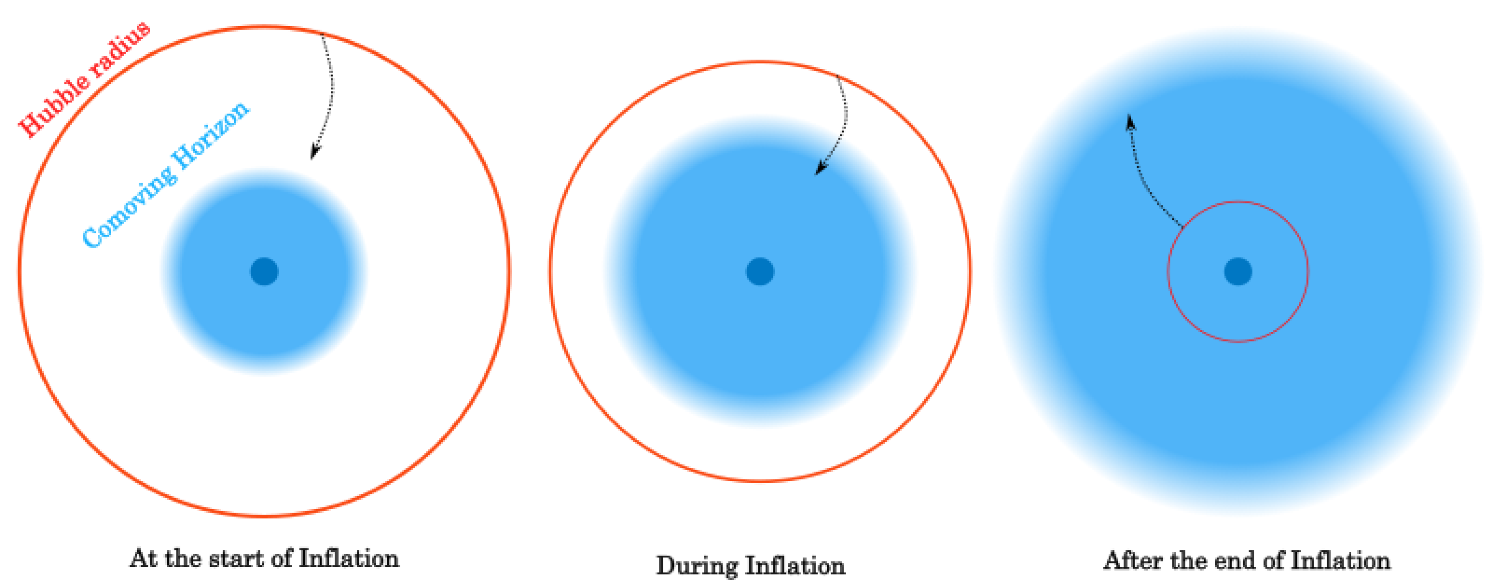
Table 1.
Factor for various modified theories of gravity. Here, is as usual the deceleration parameter.
Table 1.
Factor for various modified theories of gravity. Here, is as usual the deceleration parameter.
| Model | |
|---|---|
| Gauss–Bonnet | |
| Constrained Gauss–Bonnet | |
| String Corrections | |
| Constrained String Corrections | |
| Chern–Simons |
Disclaimer/Publisher’s Note: The statements, opinions and data contained in all publications are solely those of the individual author(s) and contributor(s) and not of MDPI and/or the editor(s). MDPI and/or the editor(s) disclaim responsibility for any injury to people or property resulting from any ideas, methods, instructions or products referred to in the content. |
© 2023 by the authors. Licensee MDPI, Basel, Switzerland. This article is an open access article distributed under the terms and conditions of the Creative Commons Attribution (CC BY) license (https://creativecommons.org/licenses/by/4.0/).
Share and Cite
MDPI and ACS Style
Odintsov, S.D.; Oikonomou, V.K.; Giannakoudi, I.; Fronimos, F.P.; Lymperiadou, E.C. Recent Advances in Inflation. Symmetry 2023, 15, 1701. https://doi.org/10.3390/sym15091701
AMA Style
Odintsov SD, Oikonomou VK, Giannakoudi I, Fronimos FP, Lymperiadou EC. Recent Advances in Inflation. Symmetry. 2023; 15(9):1701. https://doi.org/10.3390/sym15091701
Chicago/Turabian StyleOdintsov, Sergei D., Vasilis K. Oikonomou, Ifigeneia Giannakoudi, Fotis P. Fronimos, and Eirini C. Lymperiadou. 2023. "Recent Advances in Inflation" Symmetry 15, no. 9: 1701. https://doi.org/10.3390/sym15091701
Note that from the first issue of 2016, this journal uses article numbers instead of page numbers. See further details here.