
Pseudo-Finsler Radially Symmetric Spaces

1
Instituto de Matemática, Universidade Federal do Rio de Janeiro, Cidade Universitária, Rio de Janeiro 21941, Brazil
2
Departamento de Matemáticas, Universidad de Murcia, Campus de Espinardo, 30100 Murcia, Spain
*
Author to whom correspondence should be addressed.
†
These authors contributed equally to this work.
Symmetry 2024, 16(3), 362; https://doi.org/10.3390/sym16030362
Submission received: 31 January 2024
/
Revised: 3 March 2024
/
Accepted: 15 March 2024
/
Published: 18 March 2024
(This article belongs to the Special Issue Recent Advance in Mathematical Physics II)
Abstract
:We introduce the concept of radially symmetric pseudo-Finsler spaces, which generalize the notion of symmetric Finsler spaces, and prove that this concept is equivalent to the preservation of flag curvature by parallel transport together with reversibility. As a consequence, reversible pseudo-Finsler manifolds with constant flag curvature are radially symmetric.
1. Introduction
The theory of symmetric spaces was successfully developed by E. Cartan in the 1920s (see [1,2]). The concept is very simple: a complete Riemannian space is symmetric if for all , the map , such that for all geodesic and all , is an isometry. Locally, this is equivalent to M having a parallel curvature tensor, and the term locally symmetric has been reserved for the spaces with this property. The notion of symmetric space makes sense in the Finslerian realm, but it has been proved that in the global case, there is little novelty, as globally symmetric Finsler spaces (with positive definite fundamental tensors throughout) are of Berwald type (their geodesics can be computed as the auto-parallel curves of an affine connection), and there is a Riemannian symmetric space with the same geodesics (see [3], Theorem 2.7). Regarding the local case, as observed by Egloff (see the comments in [4] and also [5]), a non-Riemannian Hilbert geometry provides a counterexample of a reversible Finsler metric with parallel curvature (in the sense that we will explain later), which is not locally symmetric; namely, it does not locally admit an isometry map as defined above. Moreover, it seems that this concept of local symmetry is very restrictive and, in many cases, assuming some conditions on the flag curvature implies that the metric is Riemannian or Berwald (see [4,6,7,8]). For the study of Berwald symmetric spaces, see [3,9,10].
The main goal of this paper is to introduce a weaker notion of Finsler symmetric spaces, the so-called radially symmetric spaces, namely, those spaces with the property that the map defined above is an isometry for the osculating metrics tangent to the radial geodesics from p (see Definition 6). Then, we prove that these spaces can be characterized by being reversible with flag curvature preserved by the parallel transport. At this point, it is important to point out that to define the parallel transport of the flag curvature, it is necessary to consider the parallel transport introduced in [11]. In this way, the flagpole is transported as an observer (taking as a reference the same vector field), while the transverse edge of the flag is transported with respect to the parallel observer determined by the flagpole (see Section 2.3). Unlike the Riemannian case, this condition does not imply that some data in the tangent map, namely, the curvature tensor and the Finsler metric, completely determines the Finsler metric in a neighborhood. Indeed, the Cartan–Ambrose–Hicks type theorem in Theorem 1 only provides information about the radial directions (compare this theorem with the one given in ([12], Theorem 2.1) without a complete proof). However, assuming that the metric is Berwald, we again recover this property (see Corollary 4).
To develop all the computations, we use the notion of anisotropic connection introduced in [13] rather than the more standard approach followed in [14]. The reasons for this choice will be explained at the beginning of Section 2. We organize the paper as follows: in Section 2, we define the concept of the anisotropic tensor field and introduce the notion of anisotropic connection and how it acts on anisotropic tensor fields. In Section 2.2, we introduce the curvature tensor of an anisotropic connection. In Section 2.3, we define the two types of parallel transport along a given curve, the observer-parallel transport of an admissible vector v with respect to an anisotropic connection and the parallel transport of a vector field along the curve with respect to a chosen admissible vector v. In the final Section 3, we prove in Proposition 3 that the Jacobi curvature operator is parallel if and only if it takes a parallel vector field into another parallel vector field in both cases with respect to an observer-parallel vector field V, and this is also equivalent to the flag curvature being invariant under parallel transport. To conclude this section, we prove the Cartan–Ambrose–Hicks type result mentioned in the beginning, a characterization of being radially symmetric as being reversible with parallel Jacobi operator (Corollary 2), and finally we prove that radially symmetric is equivalent to locally symmetric for Berwald metrics (Corollaries 4 and 5).
2. Anisotropic Tensor Calculus and Pseudo-Finsler Geometry
The anisotropic tensor calculus is an attempt to make computations in Finsler geometry closer to the techniques used in modern Riemannian geometry. Its origin dates back to the use of the osculating metric by A. Nazim [15] as early as 1936 in his Ph.D. thesis. A few years later, O. Varga [16] further studied the osculating metric and its Levi–Civita connection, which turned out to admit a good interpretation when a geodesic vector field V was chosen. In 1980, H. Matthias in his Ph.D. thesis [17] took a step forward defining the so-called family of affine connections constructed from the Chern connection, which is a connection on the vertical bundle, and a choice of a vector field V without zeroes. The use of this family of affine connections was clarified by Z. Shen in 2001 in his book about sprays [18], where he made clear that the family of affine connections is very useful to compute the Jacobi operator whenever the vector field V is geodesic ([18], Proposition 8.4.3). Around the same time, Álvarez-Paiva and Durán [19], Rademacher [20,21] and Kováks and Tóth [22] gave certain popularity to the consideration of the Chern connection as a family of affine connections. The notion of anisotropic tensor calculus has been recently introduced in [13,23]. Observe that a related notion of an anisotropic connection had previously appeared in ([18], Definition 7.1.1), but the notion used here is formally slightly different (see Definition 3). One of the main achievements of the anisotropic tensor calculus is that one can completely determine the Chern curvature tensor by means of affine connections without assuming that the prescribed vector field is geodesic (see Proposition 1). On the other hand, the covariant derivation of anisotropic tensor fields has a very natural interpretation using parallel transport, as explained in [11]. To obtain this interpretation, we need to define two different types of parallel transport, one which is already known, and it can be interpreted as the parallel transport of the non-linear connection, but we call it observer-parallel transport, and the another one with respect to a vector v, which takes as as reference the observer-parallel vector field obtained from v (see Definition 4). These definitions have been crucial to establishing the equivalences in Proposition 3. Even if it is possible to make all these definitions using connections on the vertical bundle of , they are very natural in the context of anisotropic tensor calculus, and as we state above, all the computations become quite similar to the modern treatment of Riemannian geometry. As this calculus is not yet a common ground in the Finslerian community, it is explained in the following. The explicit relation with the calculus using a connection in the vertical bundle is developed in ([13], Section 4.4).
Given a smooth manifold M of dimension n, with its tangent bundle and its cotangent bundle, let us denote by and the natural projections. If A is an open subset of the tangent bundle , the restriction can be used to obtain two vector bundles over A by lifting and , which we denote, respectively, by and :
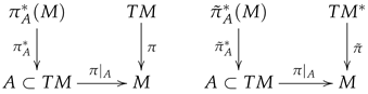
In particular, for every , one has that and . Then, a section of (resp. ) is a smooth map (resp. ) such that (resp. ). We will denote by the space of (smooth) sections of , while the subset of smooth sections of will be denoted by .
Definition 1.
An A-anisotropic tensor field T of type , , is defined as an -multilinear map
where is the subset of smooth real functions on A, namely, .
The space of A-anisotropic tensor fields of type is denoted by , while by convention . The -multilinearity implies that for every , T determines a multilinear map
By the -multilinearity, it is enough to define the tensor field as
which then will be extended by -multilinearity using a local frame in (resp. ); see also ([13], Remark 2).
One can also consider an -multilinear map
which determines the A-anisotropic tensor field of type defined by
As in classical tensor calculus, T will be considered as a tensor field itself, using the formula above only when necessary.
We will say that a vector field V defined on an open subset is A-admissible (with ) if for every . In such a case, we can define a (classical) tensor field as a map
such that
where and and denote, respectively, the space of vector fields and one-forms on .
As a result of the dependence on directions of A-anisotropic tensor fields, one can define derivatives on the vertical bundle.
Definition 2.
Given an anisotropic tensor field , its vertical derivative is defined as the tensor field given by
for any and , and an analogous definition is made for anisotropic tensor fields of the type (2).
2.1. Anisotropic Connections
Let us introduce a central concept to make operations with anisotropic tensor fields.
Definition 3.
An anisotropic (linear) connection is a map
such that
- (i)
- , for any ,
- (ii)
- for any , ,
- (iii)
- , for any , ,
where .
We will use the notation . Furthermore, the torsion of ∇ is defined as the anisotropic tensor
An anisotropic connection is said to be torsion-free if . Given a system of coordinates of M, we define the Christoffel symbols of ∇ as the functions determined by . Observe that ∇ is torsion-free if and only if is symmetric in i and j.
An anisotropic connection ∇ induces an anisotropic tensor derivation for every vector field (see [13], Section 2.2, for the general definition) in the space of anisotropic tensor fields such that for any function , is determined by
where V is any A-admissible vector field extending v, namely, . Observe that the expression in (5) does not depend on the choice of V (see [13], Lemma 9). Moreover, if is a one-form, then is determined by
Finally, for an arbitrary anisotropic tensor field , we define the derivation
for any (see [13], Theorem 11, and recall that is an anisotropic derivation as in [13], Definition 8). Observe that the same formula (7) with also holds for tensor fields of the type (2).
Finally, we can also define the vertical derivative of ∇ as the anisotropic tensor field given by:
where and are arbitrary smooth vector fields on M. Moreover, in a natural system of coordinates of the tangent bundle , associated with a coordinate system on M, one has
for every , and and and being the coordinates of . As usual, we denote the coordinates of a point as
and we use the Einstein summation convention when possible, omitting the coordinate functions and to avoid clutter in equations. Thus, P is symmetric in the first two arguments if ∇ is torsion-free.
2.2. Curvature Tensor
It is possible to associate a curvature tensor with every anisotropic (linear) connection ∇ as follows
for any and . Here, one has to take into account that , namely, they are anisotropic vector fields. One can check that R is an -multilinear map, and then an anisotropic tensor as in (2), which is anti-symmetric in X and Y.
Recall that given an A-admissible vector field V in , the anisotropic connection ∇ provides an affine connection on defined as for any , being . This affine connection determines its curvature tensor as
where are arbitrary smooth vector fields on . The tensor depends on the choice of V, but it can be used to get an expression of the curvature tensor of ∇.
Proposition 1.
Let ∇ be an anisotropic (linear) connection and , an open subset. Then, for any ,
where , V being an A-admissible extension of v.
Proof.
See [23], Proposition 2.5. □
2.3. Parallel Transport
Proposition 2.
Given a smooth curve , an anisotropic connection ∇ on M with admissible domain and an A-admissible vector field X along α, there exists a unique covariant derivative
such that whenever for some vector field Y on M.
Proof.
See [23], Proposition 2.7. □
Definition 4.
Given a regular curve , the observer-parallel transport of an admissible vector with respect to the anisotropic connection ∇ is the map
such that , where V is the vector field along α such that and . Moreover, the parallel transport with respect to v is given by
such that , being determined by and , with V as above.
Moreover, for any tensor , interpreted as
we can obtain the covariant derivative using a curve such that , an observer-parallel vector field V, with and parallel vector fields with respect to v. It turns out that
(see [11], Section 7).
2.4. Pseudo-Finsler Manifolds and Flag Curvature
We say that a function is a pseudo-Finsler metric if
- It is smooth on ;
- It is positive homogeneous of degree 2;
- For every , the fundamental tensor defined asis a non-degenerate bilinear form.
Given a pseudo-Finsler manifold, there is a unique anisotropic connection ∇ such that it is torsion-free and , (see [13], Section 4.1). This connection can be identified with the Chern connection, which can be naturally interpreted as an anisotropic connection. Using the Chern connection and its associated curvature tensor introduced in (10), one can then introduce one of the main geometrical invariants of a pseudo-Finsler metric, the flag curvature, , which depends on a vector v, which plays the role of the flagpole, and a -nondegenerate plane that contains v and w. It is defined as
Definition 5.
The flag curvature is said to be invariant under parallel translation along a curve if
for all and . When it is invariant along any regular curve, we will simply refer to it as invariant under parallel translation.
3. Radially Symmetric Finsler Manifolds
Definition 6.
Let be a pseudo-Finsler manifold with a given point and Ω a neighborhood of p with the following property: for any geodesic γ with , we have that if , then γ is defined at least in . Then,
- 1.
- We define as , where γ is the only unit geodesic such that and .
- 2.
- We say that is locally radially symmetric if for all and Ω as above, we have thatis an isometry (as above γ is a unit geodesic, and ) for all .
Recall that the Jacobi curvature operator is defined as with .
Proposition 3.
Given a pseudo-Finsler manifold, the following conditions are equivalent:
- (i)
- .
- (ii)
- If V is an observer-parallel vector field along a regular curve α and X is parallel with respect to V, then is also parallel with respect to V along α.
- (iii)
- Flag curvature is invariant under parallel translation.
Proof.
. It follows from the characterization of the covariant derivative in terms of parallel vector fields. Indeed, given a regular curve , a vector field Y such that and an observer-parallel vector field V along with , then
taking into account (12).
. Observe that if is a regular curve, V is an observer-parallel vector field with and X is a parallel vector field with respect to v, then, by applying ([23], Equation (46)), and using that , and are constant as a consequence of the choice of V and X as observer-parallel and parallel vector fields, respectively, we deduce that
as required.
. We have to check that if V is an observer-parallel vector field and X is parallel with respect to V, then for all W parallel with respect to V, but this is equivalent to proving that
is constant along (with as in the proof of ). As is constant because V is observer-parallel and X is parallel with respect to V, we have that is constant because, by hypothesis in part , the flag curvature
is constant (see the centered formula in the above implication). In particular, is also constant (as is parallel with respect to V), and therefore, we conclude that
is also constant, as required. □
Corollary 1.
A pseudo-Finsler manifold of constant flag curvature has a parallel Jacobi curvature operator.
Observe that using Proposition 3 and ([24], Theorem 2), it follows that the property of having a flag curvature invariant by parallel transport is invariant under Zermelo deformations using a killing field. Recall that a Zermelo deformation of a Finsler metric F with a vector field W is obtained as the Finsler metric Z, which has as indicatrix the translation of the indicatrix of with at each point .
Definition 7.
Let and be pseudo-Finsler manifolds and an isometry. Let us denote with the exponential map of M at p and the exponential map of at q, and let be a normal neighborhood of p small enough such that is contained in a domain of where it is a diffeomorphism. Then, we define the polar map as
The next theorem is a local Finslerian version of the Cartan–Ambrose–Hicks Theorem using the osculating metrics (see [1,2] for the original local version by Cartan and [25,26] for the global extensions).
Theorem 1.
If and are pseudo-Finsler manifolds that have parallel Jacobi curvature operators, and is a linear isometry that preserves the Jacobi curvature operator, then is an isometry with respect to the osculating metrics and , V being the tangent vector to the unit radial geodesics from p and .
Proof.
Let and denote . Then, is the radial geodesic with and . By the definition of , we have that is the radial geodesic in starting at q and with initial velocity . The tangent vector V to is an observer-parallel vector field, i.e., . Similarly, the tangent vector field to the geodesic is an observer-parallel vector field, i.e., .
To show that is an isometry with respect to the osculating metrics and , it suffices to show that for any , with for , we have .
We know, from the description of Jacobi fields using the exponential map (see, for example, [27], Lemma 3.14 and Proposition 3.15) that for some , and then , where is the unique Jacobi field with and (here using ).
Now, we look at the manifold . Since ; therefore, and together with the fact that , since ℓ is linear, gives that , where is the unique Jacobi field with and .
Let be an orthonormal basis of with regard to the metric and let be its parallel transport with respect to v along . This parallel frame will be orthonormal with regard to the metric . Since ℓ is a linear isometry, is an orthonormal basis of with regard to the metric . Let be its parallel transport with regard to the vector along the geodesic . This parallel frame will remain parallel with regard to the metric , and we have that .
We write , which gives . Similarly, if , then . We also write the Jacobi fields Z along and along using these parallel frames as and , respectively. They satisfy the Jacobi field equation , which can be written as , where is the Jacobi operator. So, the coordinate functions satisfy the system of ODEs
where . Since is parallel and V is the observer-parallel translation of v, it follows that is constant, since by Proposition 3, is also parallel. A similar argument, using the Jacobi equation satisfied by on the manifold , gives
where and is the Jacobi operator associated with . Since is parallel and is the observer-parallel translation of , it follows that the components are also constant. However, on the common domain I, since the isometry ℓ preserves the Jacobi curvature operator, i.e., at .
It follows that the functions and , satisfy the same system of linear ODEs with the same initial conditions, so it follows by uniqueness of such solutions that . Therefore , where for . □
Corollary 2.
A reversible pseudo-Finsler manifold has parallel Jacobi operator if and only if it is locally radially symmetric.
Proof.
As is reversible, at every point , the map , is an isometry. Moreover, the reversibility also implies that ℓ preserves the Jacobi operator, namely, for all , and then we can apply Theorem 1 to conclude the implication to the right. For the converse, observe that the radial isometry preserves , and therefore
for any , since . As , because F is reversible, we also have that , and then we conclude that . □
Corollary 3.
A reversible pseudo-Finsler metric with constant flag curvature is locally radially symmetric.
Proof.
A constant flag curvature manifold always satisfies part (iii) of Proposition 3, and then it has a parallel Jacobi operator. Therefore, the result follows from Corollary 2. □
In particular, Hilbert geometries are always radially symmetric, as they have constant flag curvature and are reversible. Recall that a Hilbert–Finsler metric is defined by symmetrizing a Berwald metric, which is obtained applying a Zermelo deformation with the position vector field to the unit ball of a Minkowski norm.
Corollary 4.
If and are Berwald manifolds that have parallel Jacobi curvature operator, and is an isometry that preserves the Jacobi curvature operators, then is an isometry.
Proof.
Observe that as is Berwald, and V is the tangent vector field to the unit geodesics from a certain , then the anisotropic connection is indeed an affine connection on M and coincides with the Chern connection of L (see [18], p. 100). Moreover, as V is geodesic, is the Levi–Civita connection of , and then , where is the tangent vector field to the unit geodesics from , since is an isometry of and , the osculating metrics of and , respectively. Finally, using that the parallel transport of ∇ preserves the Berwald metric L and that ℓ also preserves L, we easily conclude that is an isometry for L and (see also [28], Theorem 5.2). □
Corollary 5.
If is a reversible Berwald manifold that has a parallel Jacobi curvature operator, then it is locally symmetric.
4. Conclusions
In this paper, we have introduced the class of locally radially symmetric pseudo-Finsler manifolds, a new family of pseudo-Finsler manifolds with some symmetric properties with respect to an osculating metric associated with the exponential map. The advantage of this family with respect to the classical symmetric Finsler manifolds is that these metrics can be characterized as those which are reversible and have parallel flag curvature (see Corollary 2), mimicking what occurs in the family of locally symmetric Riemannian manifolds. Moreover, they include reversible pseudo-Finsler manifolds with constant flag curvature (see Corollary 3). The key result to prove all these properties is Theorem 1, which is a Cartan–Ambrose–Hicks Theorem, and it does not hold in general when the isometry of the osculating metrics is replaced with an isometry of the pseudo-Finsler metrics.
Author Contributions
The authors have all contributed substantially to the derivation of the presented results as well as analysis, drafting, review and finalization of the manuscript. All authors have read and agreed to the published version of the manuscript.
Funding
M.A.J. was partially supported by the project PID2021-124157NB-I00, funded by MCIN/AEI/10.13039/501100011033/“ERDF A way of making Europe”, and also by Ayudas a proyectos para el desarrollo de investigación científica y técnica por grupos competitivos (Comunidad Autónoma de la Región de Murcia), included in the Programa Regional de Fomento de la Investigación Científica y Técnica (Plan de Actuación 2022) of the Fundación Séneca-Agencia de Ciencia y Tecnología de la Región de Murcia, REF. 21899/PI/22.
Data Availability Statement
Data are contained within the article.
Conflicts of Interest
The authors declare no conflicts of interest.
References
- Cartan, É. Sur une classe remarquable d’espaces de Riemann, I. Bull. Soc. Math. Fr. 1926, 54, 214–216. [Google Scholar] [CrossRef]
- Cartan, É. Sur une classe remarquable d’espaces de Riemann, II. Bull. Soc. Math. Fr. 1927, 55, 114–134. [Google Scholar] [CrossRef]
- Deng, S.; Hou, Z. On symmetric Finsler spaces. Isr. J. Math. 2007, 162, 197–219. [Google Scholar] [CrossRef]
- Foulon, P. Locally symmetric Finsler spaces in negative curvature. C. R. Acad. Sci. Paris Sér. I Math. 1997, 324, 1127–1132. [Google Scholar] [CrossRef]
- Egloff, D. Some New Developments in Finsler Geometry. Ph.D. Dissertation, University Fribourg, Fribourg, Switzerland, 1995. [Google Scholar]
- Kim, C.-W. Locally symmetric positively curved Finsler spaces. Arch. Math. 2007, 88, 378–384. [Google Scholar] [CrossRef]
- Matveev, V.S. There exist no locally symmetric Finsler spaces of positive or negative flag curvature. C. R. Math. Acad. Sci. Paris 2015, 353, 81–83. [Google Scholar] [CrossRef]
- Wu, B.Y. Some rigidity theorems for locally symmetrical Finsler manifolds. J. Geom. Phys. 2008, 58, 923–930. [Google Scholar] [CrossRef]
- Deng, S.; Hou, Z. On locally and globally symmetric Berwald spaces. J. Phys. A Math. Gen. 2005, 38, 1691–1697. [Google Scholar] [CrossRef]
- Deng, S.; Hou, Z. Minkowski symmetric Lie algebras and symmetric Berwald spaces. Geom. Dedicata 2005, 113, 95–105. [Google Scholar] [CrossRef]
- Javaloyes, M.Á.; Sánchez, M.; Villaseñor, F.F. Anisotropic connections and parallel transport in Finsler spacetimes. In Developments in Lorentzian Geometry; Springer Proceedings in Mathematics & Statistics Series; Springer: Cham, Switzerland, 2022; Volume 338, 32p, ISBN 978-3-031-05378-8. [Google Scholar]
- Abate, M.; Patrizio, G. Finsler metrics of constant curvature and the characterization of tube domains. Contemp. Math. 1996, 196, 101–107. [Google Scholar]
- Javaloyes, M.A. Anisotropic tensor calculus. Int. J. Geom. Methods Mod. Phys. 2019, 16, 1941001. [Google Scholar] [CrossRef]
- Bao, D.; Chern, S.-S.; Shen, Z. An Introduction to Riemann-Finsler Geometry; Springer: New York, NY, USA, 2000; Volume 200. [Google Scholar]
- Nazim, A. Über Finslersche Räume; Wolf: München, Germany, 1936. [Google Scholar]
- Varga, O. Zur Herleitung des invarianten Differentials in Finslerschen Räumen. Monatsh. Math. Phys. 1941, 50, 165–175. [Google Scholar] [CrossRef]
- Matthias, H.-H. Zwei Verallgemeinerungen eines Satzes von Gromoll und Meyer; Bonner Mathematische Schriften [Bonn Mathematical Publications]; Universität Bonn Mathematisches Institut: Bonn, Germany, 1980; Volume 126. [Google Scholar]
- Shen, Z. Differential Geometry of Spray and Finsler Spaces; Kluwer Academic Publishers: Dordrecht, The Netherlands, 2001. [Google Scholar]
- Álvarez Paiva, J.C.; Durán, C.E. Isometric submersions of Finsler manifolds. Proc. Am. Math. Soc. 2001, 129, 2409–2417. [Google Scholar] [CrossRef]
- Rademacher, H.-B. Nonreversible Finsler metrics of positive flag curvature. In A Sampler of Riemann-Finsler Geometry; Cambridge University Press: Cambridge, UK, 2004; Volume 50, pp. 261–302. [Google Scholar]
- Rademacher, H.-B. A sphere theorem for non-reversible Finsler metrics. Math. Ann. 2004, 328, 373–387. [Google Scholar] [CrossRef]
- Kovács, Z.; Tóth, A. On the geometry of two-step nilpotent groups with left invariant Finsler metrics. Acta Math. Acad. Paedagog. Nyházi. 2008, 24, 15–168. [Google Scholar]
- Javaloyes, M.A. Curvature computations in Finsler geometry using a distinguished class of anisotropic connections. Mediterr. J. Math. 2020, 17, 21. [Google Scholar] [CrossRef]
- Foulon, P.; Matveev, M.S. Zermelo deformation of Finsler metrics by Killing vector fields. Electron. Res. Announc. Math. Sci. 2018, 25, 1–7. [Google Scholar] [CrossRef]
- Ambrose, W. Parallel Translation of Riemannian Curvature. Ann. Math. 1956, 64, 337. [Google Scholar] [CrossRef]
- Hicks, N. A theorem on affine connexions. Ill. J. Math. 1959, 3, 24–254. [Google Scholar] [CrossRef]
- Javaloyes, M.A.; Soares, B.L. Geodesics and Jacobi fields of pseudo-Finsler manifolds. Publ. Math. Debr. 2015, 87, 57–78. [Google Scholar] [CrossRef]
- Deng, S. Homogeneous Finsler Spaces; Springer Monographs in Mathematics; Springer: New York, NY, USA, 2012; 240p. [Google Scholar]
Disclaimer/Publisher’s Note: The statements, opinions and data contained in all publications are solely those of the individual author(s) and contributor(s) and not of MDPI and/or the editor(s). MDPI and/or the editor(s) disclaim responsibility for any injury to people or property resulting from any ideas, methods, instructions or products referred to in the content. |
© 2024 by the authors. Licensee MDPI, Basel, Switzerland. This article is an open access article distributed under the terms and conditions of the Creative Commons Attribution (CC BY) license (https://creativecommons.org/licenses/by/4.0/).
Share and Cite
MDPI and ACS Style
Ionel, M.; Javaloyes, M.Á. Pseudo-Finsler Radially Symmetric Spaces. Symmetry 2024, 16, 362. https://doi.org/10.3390/sym16030362
AMA Style
Ionel M, Javaloyes MÁ. Pseudo-Finsler Radially Symmetric Spaces. Symmetry. 2024; 16(3):362. https://doi.org/10.3390/sym16030362
Chicago/Turabian StyleIonel, Marianty, and Miguel Ángel Javaloyes. 2024. "Pseudo-Finsler Radially Symmetric Spaces" Symmetry 16, no. 3: 362. https://doi.org/10.3390/sym16030362
Note that from the first issue of 2016, this journal uses article numbers instead of page numbers. See further details here.