A Novel Money Laundering Prediction Model Based on a Dynamic Graph Convolutional Neural Network and Long Short-Term Memory

Abstract

Money laundering is an illicit activity that seeks to conceal the nature and origins of criminal proceeds, posing a substantial threat to the national economy, the political order, and social stability. To scientifically and reasonably predict money laundering risks, this paper focuses on the “layering” stage of the money laundering process in the field of supervised learning for money laundering fraud prediction. A money laundering and fraud prediction model based on deep learning, referred to as MDGC-LSTM, is proposed. The model combines the use of a dynamic graph convolutional network (MDGC) and a long short-term memory (LSTM) network to efficiently identify illegal money laundering activities within financial transactions. MDGC-LSTM constructs dynamic graph snapshots with symmetrical spatiotemporal structures based on transaction information, representing transaction nodes and currency flows as graph nodes and edges, respectively, and effectively captures the relationships between temporal and spatial structures, thus achieving the dynamic prediction of fraudulent transactions. The experimental results demonstrate that compared with traditional algorithms and other deep learning models, MDGC-LSTM achieves significant advantages in comprehensive spatiotemporal feature modeling. Specifically, based on the Elliptic dataset, MDGC-LSTM improves the Macro-F1 score by 0.25 compared to that of the anti-money laundering fraud prediction model currently considered optimal.

1. Introduction

Money laundering refers to the process of disguising, concealing, and transforming illicitly obtained funds through a series of legal or seemingly legal economic transactions [1]. The purpose of this behavior is to obscure the true origins of funds, making them appear to have come from legitimate channels, thus evading legal tracking and regulatory oversight by law enforcement agencies [2]. The negative impacts of money laundering on society are multifaceted. First, money laundering facilitates the legitimization of funds from criminal activities, thereby increasing the sustainability and scale of criminal operations. This not only enables criminals to continue engaging in illicit activities but also may lead to worsening public safety and rising crime rates. Second, money laundering disrupts the normal economic order, subjecting legitimate businesses and individuals to an unfair competitive environment. Since money launderers typically utilize legitimate enterprises or transactions for fund laundering, this distorts market prices, undermining the fairness and transparency of the economy.

In recent years, digital financial technology has led to an extensive transformation of the financial sector, offering more efficient, convenient, and innovative services [3]. Digital financial technology utilizes advanced digital and information technologies, including blockchain technology, artificial intelligence, big data analytics, and cloud computing, thus altering and optimizing traditional financial services and transaction methods [4]. While the development of digital financial technology has brought convenience to our lives, it has also triggered a range of societal issues, one of which is digital money laundering. Criminals exploit the anonymity of digital financial transactions and the automatic execution of smart contracts to engage in complex money laundering schemes [5]. The global nature of digital financial transactions, along with the liquidity of virtual assets and cryptocurrencies, has increased the difficulty of tracking and law enforcement [6]. From the beginning to the end of 2017, the total cryptocurrency market value increased from just $18 billion to more than $600 billion [7]. Recent reports have highlighted cases in northern Myanmar where telecommunications fraudsters engaged in money laundering through property purchases in Singapore, virtual currency transactions, encrypted payments, and online payments. Consequently, money laundering prediction has become a crucial component of the national security strategy employed in this new era.

Traditional money laundering prediction methods rely on a series of detection, identification, and reporting procedures to assist financial institutions and regulatory authorities in detecting suspicious transactions and taking appropriate countermeasures [8]. However, with the continuous advancement of technology, emerging digital financial technologies and intelligent criminal methods have also propelled innovation in money laundering prediction technologies [9]. Statistical methods and machine learning methods are playing increasingly important roles in money laundering prediction strategies and are currently the most widely used approaches in the field. Statistical methods include rule-based screening [10], descriptive statistics [11,12], time series analysis [13], and collaborative filtering [14]. Machine learning methods include heuristic algorithms [15], logistic regression [16,17], support vector machines (SVMs) [18,19], ensemble learning [20], and multilayer perceptrons (MLPs) [21]. In recent years, the rapid development of deep learning, especially because of its outstanding ability to automatically extract features, has led to its widespread application in financial risk prediction scenarios.

Money laundering transactions often exhibit characteristics such as short-term frequent small transactions, unusual transaction timings, sudden large transactions, and periodic transactions. These features reveal patterns, trends, and cyclical time series characteristics in transaction time sequences. Due to their excellent sequence modeling capabilities, recurrent neural networks (RNNs) [22] can effectively capture the temporal dependencies in input data. To overcome the issues faced by traditional RNNs when handling long sequences, improved structures such as long short-term memory (LSTM) [23,24,25] and gated recurrent units (GRUs) [26,27,28] have been proposed, achieving better results in tasks involving time series data.

Money laundering transactions involve complex currency flow paths, forming specific connection patterns that constitute a graph network structure of money laundering transactions. Graph convolutional neural networks (GCNs) [29,30,31,32,33,34,35,36] are effective methods for capturing node connection relationships by aggregating similar nodes to form spatially meaningful node clusters, aiding in the discovery of potential money laundering patterns. Graph convolution can also explain information transmission patterns between nodes, helping identify potential paths in money laundering activities.

However, considering that money laundering transactions possess both temporal and spatial structural features, the use of a single model for feature extraction has limitations. Recent research [33,34] has indicated that deep neural network approaches that integrate both temporal and spatial features can achieve outstanding performance in terms of predicting money laundering transactions. The method proposed in [33] achieved a prediction accuracy of more than 96% based on the Elliptic dataset for predicting money laundering transactions. Nevertheless, the current research relies primarily on the static design of money laundering transaction graphs and uses static graphs for graph convolution purposes in dynamic time series prediction tasks, leading to issues such as dynamic temporal feature neglect and information leakage. Recent studies [37,38] have proposed an innovative approach in this context, introducing a time attribute based on static graphs and transforming them into dynamic graphs based on timestamps to enhance the predictive performance of the constructed model and mitigate the potential risk of excessive smoothing. The neural network architecture constructed based on the time-series dynamic model consistently exhibits symmetrical properties at each time step, ensuring persistent symmetry in the model, which in turn guarantees its robustness and credibility.

In summary, the main contributions of this paper are as follows.

(1)

A novel prediction model that integrates dynamic graph convolution and LSTM is proposed to address the shortcomings of the previous models in terms of capturing the dynamic spatial features contained in the static graph consisting of all transactions.

(2)

A dynamic graph convolution method is constructed based on snapshots to reduce the risk of excessively smoothing the transaction nodes.

(3)

Comprehensive experimental studies are conducted to significantly improve the performance of the proposed money laundering prediction model.

2. Related Works

To mitigate the harm caused by money laundering transactions, many scholars have attempted to use statistical methods and traditional machine learning methods for predicting the risks associated with such transactions. However, rule-based methods [10] are often constrained by predefined rule sets, making it challenging for such models to adapt to new money laundering patterns. Descriptive statistical methods [11,12] mainly focus on overall data characteristics, but in money laundering prediction tasks, they may overlook the details of individual anomalous transactions, making it challenging to capture the complex relationships between different transactions. Time series analysis [13] performs well in terms of handling periodic money laundering patterns but struggles to capture the nonlinear relationships between transactions exhibiting complex nonperiodic patterns. Heuristic algorithms [15], limited by their manually designed heuristic rules, face challenges when attempting to automatically learn more abstract and complex patterns in large-scale and high-dimensional datasets. Logistic regression [16,17], which is a linear model, has a limited ability to model complex nonlinear relationships. SVMs [18,19] exhibit good fitting capabilities in high-dimensional spaces but are time-consuming when trained on large datasets and relatively limited regarding modeling temporal and spatial relationships. The performance of ensemble learning [20] strongly depends on the diversity of the base learners and requires significant effort for parameter tuning and selection. The performance of an MLP [21] is restricted by the input data volume and the required training time, and MLPs struggle to capture the higher-order spatiotemporal relationships among money laundering transactions.

In recent years, the rapid development of deep learning technology has positioned deep learning models as powerful tools in the field of financial risk prediction. Deep learning models possess advantages such as automatically learning abstract features from data, being suitable for handling high-dimensional and large-scale data, and supporting end-to-end learning. Consequently, several scholars have applied deep learning techniques to financial risk prediction. Financial transactions usually exhibit temporal characteristics, and deep neural networks based on RNNs have inherent advantages in terms of extracting temporal features. LSTM, an RNN variant, is well suited for extracting features from datasets formed in a big data environment. Alghofaili Y et al. [24] proposed a deep learning fraud detection method based on LSTM, which achieved outstanding performance in credit card fraud detection applications. Yan et al. [25] introduced an innovative deep prediction model that combines LSTM with empirical mode decomposition (EMD) and principal component analysis (PCA), achieving good stock market prediction results. A GRU is another RNN algorithm known for its higher computational efficiency than that of LSTM. Luo et al. [27] demonstrated the effectiveness of using a GRU to extract deep temporal features from information flows, contributing to the exploration of dynamic temporal dataset features. Labanca D et al. [28] proposed using a GRU to automatically extract implicit temporal features from bank transaction data and built a fusion model with features extracted using self-attention mechanisms as an alternative to traditional rule-based methods. Additionally, several works have proposed using transformer models [39], which were originally designed for processing language sequences and have achieved good results. Tatulli M P et al. [40] adopted a hierarchical transformer, introducing attention mechanisms at both the transaction and temporal levels, and achieved excellent fraud transaction detection results.

During financial transactions, currency flows between transactions, allowing for the construction of financial transaction graphs. Different spatial structure features exist among different transaction nodes based on edge relationships. The spatial structure features of financial transactions can be explored to effectively complement the limitations encountered when exploring only temporal features. Early works used GCNs for spatial structure feature mining and achieved better predictive performance than random forests [29]. In recent years, research on graph neural networks (GNNs) has gained widespread attention, with many scholars dedicated to optimizing them. You et al. [30] addressed the expression limitations of homogeneous graph message passing and proposed an innovative method that implements multi-round heterogeneous message passing. Additionally, Li et al. [31] incorporated key technologies derived from convolutional neural networks (CNNs), such as residual connections and dilated convolutions, into a GCN, successfully constructing a deep GCN with up to 112 layers. Through validations conducted on specific datasets and tasks, the authors demonstrated the effectiveness of this approach.

The use of a single model for feature extraction may not fully capture the diversity and abstraction levels in complex data, limiting the ability of the model to effectively represent comprehensive information. Considering the feature extraction limitations of a single model, Luo et al. [27] proposed merging different neural networks to produce a model with an enhanced ability to comprehensively learn features, thereby further improving the performance of the prediction model. Xia et al. [33] and Alarab et al. [34] successively proposed using a GCN to explore spatial structure features in transactions and then transferring the mined features to LSTM for temporal feature extraction. The constructed fusion network exhibited significantly better money laundering transaction prediction performance than did the single models. Huang H et al. [41] used multi-head attention mechanisms during the graph convolution process to embed spatial structures in a graph. Simultaneously, they fused this model with an LSTM model and achieved outstanding money laundering transaction prediction results.

However, the existing research is limited to representing the relationships between transaction nodes using static graphs, overlooking the inherent temporal features of timestamps. Static graphs constructed based on all transaction information suffer from information leakage issues, and after performing graph convolution operations for multiple timestamps, the resulting node features are prone to excessive smoothing. This paper addresses these challenges by constructing dynamic graph snapshots, modeling transaction information for each timestamp, utilizing an MLP layer for dynamic node updates, and integrating the results with an LSTM network to form a fusion prediction model. This fusion strategy effectively enhances the illegal transaction prediction performance of the model.

3. Construction of the MDGC-LSTM Model

To more effectively detect illicit money laundering activities in financial transactions, this paper proposes a money laundering prediction model based on a dynamic GCN and LSTM (MDGC-LSTM). Figure 1 illustrates the overall algorithmic process of MDGC-LSTM.

In the algorithmic process depicted in Figure 1, each transaction is treated as a node in a graph, and currency flows are regarded as edge relationships in the graph. The experiments in this paper focus on snapshot representations of dynamic graphs, where nodes and edges arrive in batches according to their timestamps. At each timestamp node of a transaction, the features of the transaction nodes are obtained from the transaction set of the current timestamp, and the snapshot representation of the current dynamic graph is obtained from the currency flows of the current timestamp. Within each timestamp, only one dynamic graph snapshot is retained on the GPU, and message passing is conducted solely on this dynamic graph snapshot to obtain transaction node features.

At each timestamp, graph convolution operations are initially performed to extract the spatial structural features between different transaction nodes (see Section 3.1 for details). Subsequently, these features are fed into an LSTM network to further extract the temporal features from the transaction information (see Section 3.2). Finally, the spatiotemporal features extracted by the LSTM are input into a classification network to be modeled (see Section 3.3). Each timestamp outputs a dynamic model based on the current timestamp, and the subsequent timestamp loads the model from the previous timestamp, achieving dynamic iterative updates for the model. At each timestamp, the system also outputs prediction results based on the current timestamp.

3.1. Spatial Feature Extraction

3.1.1. Message Passing and Aggregation

To more effectively identify illicit activities in money laundering transactions, each transaction in this study is considered a node in a graph, and the flow of funds between a pair of transactions is considered an edge. Thus, a graph can be represented as follows:

$$G=\left(Vertex,Eage\right)$$

(1)

where $Vertex=\{V_1,\dots ,V_n\}$ represents the set of transaction nodes and $Eage\subseteq V\times V$ represents the set of edges in the graph. Each transaction node has a corresponding feature $E_0$, which is used to represent detailed information about the transaction.

The objective of GNNs is to learn embedded representations of nodes by iteratively aggregating the information derived from the neighboring nodes within the local network. In this paper, we use an embedding matrix $E^{\left(l\right)}=\left\{E_v^{\left(l\right)}\right\}$ to represent the collection of embeddings for all nodes after applying the l-th layer of the GNN. After the nodes pass through the l-th layer of the GNN, the changes in their embedded representations can be expressed as follows:

$$E^{\left(l\right)}={GNN}^{\left(l\right)}\left(E^{\left(l-1\right)}\right)$$

(2)

Here, $E^{\left(l\right)}$ represents the collection of embeddings for all nodes after applying the l-th graph convolution layer, and ${GNN}^{\left(l\right)}$ denotes the GCN layer at the l-th level.

The graph convolution operation is essentially a series of message passing and aggregation operations within the constructed graph. In the graph convolution layer, the message passing and aggregation process for the target node can be expressed as follows:

$$\begin{array}{c}{m}_{u\to v}^{\left(l\right)}={MSG}^{\left(l\right)}\left(E_u^{\left(l-1\right)},E_v^{\left(l-1\right)}\right)\\ E_v^{\left(l\right)}={AGG}^{\left(l\right)}\left(\left\{m_{u\to v}^{\left(l\right)}|u\in N\left(v\right)\right\},E_v^{\left(l-1\right)}\right)\end{array}$$

(3)

where $E_v^{\left(l-1\right)}$ represents the embedding of the target node in layer l − 1, $E_u^{\left(l-1\right)}$ represents the embedding of the neighboring nodes in layer l − 1 that are adjacent to the target node, ${MSG}^{\left(l\right)}$ denotes the message passing function, $N\left(v\right)$ is the set of neighbors of the target node, and ${AGG}^{\left(l\right)}$ represents the message aggregation function.

During the message passing and aggregation process, different nodes may contain varying amounts of information. Therefore, during the node embedding update process, it is necessary to consider the degrees of the transaction nodes. The update rule for the node embeddings can be expressed as follows:

$$E^{\left(l\right)}=\left\{\begin{array}{cc}\sigma \left(D_v^{-\frac{1}{2}}A{D}_u^{-\frac{1}{2}}{E}^{\left(l-1\right)}{W}^{\left(l-1\right)}\right)& l\ge 1\\ E_0& l=0\end{array}\right.$$

(4)

where $D_v$ represents the input degree matrix of the target node, $D_u$ represents the output degree matrix of the neighboring nodes, $A$ represents the adjacency matrix of the target node, $E^{\left(l\right)}$ represents the embedding output of the l-th layer GNN, $W^{\left(l\right)}$ represents the feedforward network layer added after the l-th layer graph convolution, and $\sigma$ denotes the message aggregation process.

The message passing and aggregation process defined in Equation (4) is commonly referred to as a static GCN. It is designed for learning node features from a preconstructed static graph and therefore cannot capture the structural information evolving in dynamic graphs over time.

3.1.2. Dynamic Graph Snapshots

In a dynamic graph, the feature of each node includes a timestamp $S_v$, and each currency flow includes a timestamp feature $S_e$. When addressing dynamic graphs, it is necessary to construct timestamp-based dynamic graph snapshots based on the currency flows of different timestamps. A dynamic graph representing money laundering transactions can be expressed as follows:

$$G_D={\left\{G^{\left(t\right)}\right\}}_{t=1}^T$$

(5)

where $G_D$ represents a collection of graph snapshots and each snapshot $G^{\left(t\right)}=\left({Vertex}_t,{Edge}_t\right)$ is a static graph with ${Vertex}_t=\left\{v\in V|S_v=t\right\}$ and ${Edge}_t=\left\{e\in E|S_e=t\right\}$. By modeling the constructed transaction graph snapshots, automatic addition and deletion operations can be implemented on nodes according to the order of the timestamps, as different graph snapshots may contain distinct sets of nodes.

3.1.3. Dynamic Graph Convolution

A static GNN typically consists of L graph convolution layers, and the message passing and aggregation operations in each layer follow Equation (3), where $E^{\left(l\right)}$ represents the information aggregated from the neighbors within $l$ hops of the target node. The embedded values calculated at each timestamp $t$ are denoted as $E_t$. When considering only the dynamic graph convolution operation, the model fine-tuning process is as illustrated in Figure 2.

As illustrated in Figure 2, during dynamic graph convolution, at each time step $t$, the model fine-tunes the GNN using the node embeddings and labels $y_t$ of the current time step, updating the node embedding values $E_t$.

In conventional approaches [42,43,44], a temporal model built on a GNN typically retains and updates the embeddings $E^{\left(l\right)}$ of the top graph convolution layer. However, for the node states $E_t^{\left(l\right)}$ at each timestamp, the network must be retrained based on new graph snapshots. Nevertheless, the key to extending static GNNs to dynamic GNNs, as proposed in reference [37], lies in how to update the layered node states over time. Therefore, in this paper, we preserve the layered node embeddings $E_t^{\left(1\right)},\dots ,E_t^{\left(l\right)}$ for all timestamps and employ an MLP layer at each timestamp to dynamically update the node states by following the updating rule outlined below:

$$E_t^{\left(l\right)}=MLP\left(Concat\left(E_{t-1}^{\left(l\right)},E_t^{\left(l-1\right)}\right)\right)$$

(6)

where $E_{t-1}^{\left(l\right)}$ represents the embedding values of the l-th graph convolution layer at the previous timestamp and $E_t^{l-1}$ denotes the embedding output of layer l − 1 at the current timestamp.

3.2. Temporal Feature Extraction

Money laundering transactions often exhibit significant temporal dependencies, as launderers may gradually increase the sizes of their transactions and frequently change transaction partners to evade detection. Therefore, temporal feature extraction must be performed on money laundering transactions to delve into the complex temporal relationships hidden within them. LSTM is an RNN variant that was designed for sequence data; it specifically aims to capture long-term temporal dependencies. Thus, this paper employs LSTM to extract the temporal features of money laundering transactions.

LSTM introduces mechanisms such as memory units, input gates, forget gates, and output gates to address the vanishing gradient problem encountered by traditional RNNs, enabling the network to better handle long sequence data. The basic structure of LSTM is illustrated in Figure 3.

In Figure 3, the memory unit in an LSTM network is a critical network component that is responsible for storing and transmitting information. It enables the network to selectively remember or forget certain information, facilitating the better capture of long-term sequence dependencies. Additionally, the network structure of LSTM includes input gates, forget gates, and output gates. Specifically, an input gate controls how much new information is added to the memory unit, a forget gate determines which information should be deleted from the memory unit, and an output gate decides how much information is output from the memory unit. The specific structures of these gates are outlined below:

$$\begin{array}{c}\begin{array}{c}{I}_t=\sigma \left(X_t{U}_i+H_{t-1}{W}_i\right)\\ \overline{C_t}=tanh\left(X_t{U}_c+H_{t-1}{W}_c\right)\end{array}\\ \begin{array}{c}{f}_t=\sigma \left(X_t{U}_f+H_{t-1}{W}_f\right)\\ O_t=\sigma \left(X_t{U}_O+H_{t-1}{W}_O\right)\end{array}\\ \begin{array}{c}{C}_t=f_t{C}_{t-1}+I_t\overline{C_t}\\ H_t=O_t\times tanh\left(C_t\right)\end{array}\end{array}$$

(7)

where $I_t$ and $\overline{C_t}$ denote the input gate and $f_t$, $O_t$, and $C_t$ represent the forget gate, output gate, and memory unit, respectively. $H_t$ represents the output of the LSTM network at time $t$, and $X_t$ represents the feature input of the model at time $t$. $U_i$ and $U_c$ represent the weight matrices for the input gate; $U_f$ and $U_O$ represent the weight matrices for the forget gate and output gate, respectively; and $W_f$, $W_c$, $W_i$ and $W_O$ are bias terms. $\sigma$ and $tanh$ represent the sigmoid and tanh activation functions, respectively.

3.3. Modeling Spatiotemporal Features

As analyzed earlier, money laundering transactions typically exhibit both temporal and spatial structural features. The combined spatiotemporal modeling strategy using MDGC and LSTM enables the comprehensive capture of multilayered relationships in money laundering transaction data. The MDGC effectively extracts the spatial structural relationships between nodes through dynamic graph convolution operations, and the obtained spatial money laundering features are subsequently passed to the LSTM layer to capture the temporal features of the transaction data. The algorithmic process of MDGC-LSTM is summarized in Algorithm 1.

Algorithm 1 Model Based on Dynamic Graph Convolutional and LSTM (MDGC_LSTM)

Input: Dynamic Snapshot $G_D={\left\{G^{\left(t\right)}\right\}}_{t=1}^T$, Features $X_t$

Output: Prediction ${\widetilde{y_t}}^{\left(val\right)}$, MDGC_LSTM model

1: $E_t^{\left(0\right)}\leftarrow X_t^{\left(train\right)}$; //Initialize embedding from $G_D$ and $X_t$

2: for $t=1,\dots ,T$ do

3:    Load the model from the previous time step;

4:    for $l=1,\dots ,L$ do

5:         $E^{\left(l\right)}={GNN}^{\left(l\right)}\left(E^{\left(l-1\right)}\right)$; //Equation (2)

6: $E_t^{\left(l\right)}=MLP\left(Concat\left(E_{t-1}^{\left(l\right)},E_t^{\left(l-1\right)}\right)\right)$; //Equation (6)

7: $H_t=LSTM\left(E_t^{\left(l\right)}\right)$; //Equation (8)

8: ${\widetilde{y_t}}^{\left(train\right)}=Softmax\left(ReLU\left(MLP\left(H_t\right)\right)\right)$;

9: Update model via back propagation based on ${\widetilde{y_t}}^{\left(train\right)}$, $y_t^{\left(train\right)}$;

10: ${\widetilde{y_t}}^{\left(val\right)}\leftarrow EVALUATE\left(model;X_t^{\left(val\right)}\right)$

As in the design philosophy of dynamic graph convolution described in Section 3.1, at each timestamp, the model trained on the previous timestamp is loaded. Simultaneously, graph convolution operations are performed on the constructed graph snapshot using the data from the current timestamp. Based on the above analysis, the computational process of MDGC-LSTM is as follows:

$$\begin{array}{c}\begin{array}{c}{I}_t=\sigma \left(E_t^{\left(l\right)}{U}_i+H_{t-1}{W}_i\right)\\ \overline{C_t}=tanh\left(E_t^{\left(l\right)}{U}_c+H_{t-1}{W}_c\right)\\ f_t=\sigma \left(E_t^{\left(l\right)}{U}_f+H_{t-1}{W}_f\right)\end{array}\\ \begin{array}{c}{O}_t=\sigma \left(E_t^{\left(l\right)}{U}_O+H_{t-1}{W}_O\right)\\ C_t=f_t{C}_{t-1}+I_t\overline{C_t}\\ H_t=O_t\times tanh\left(C_t\right)\end{array}\end{array}$$

(8)

Here, $E_t^{\left(l\right)}$ represents the dynamic graph convolution embedding calculated at timestamp $t$ using Equation (6). In the MDGC-LSTM model, dynamic graph convolution is employed to extract the spatial features of money laundering transactions. These spatial features are subsequently conveyed to the LSTM network for further temporal characteristic extraction. After obtaining the spatiotemporal features, they are then forwarded to the fully connected layer and the output layer for classification purposes, yielding classification results for money laundering prediction.

4. Experimental Design and Analysis

4.1. Experimental Setup

4.1.1. Description of the Dataset

This study leverages two widely adopted standard graph datasets, namely, the Elliptic [16] and OGB-Arxiv [45] datasets, to serve as the experimental foundation for validating the effectiveness of the proposed methodology. The datasets are randomly partitioned into training, validation, and test sets at an 8:1:1 ratio, ensuring consistency during the partitioning process through the use of the same random seed. The Elliptic dataset has extensive applications in the domains of money laundering prevention and fraud detection. Detailed descriptions of both datasets are provided in

Table 1. Statistical information of the utilized datasets.

Dataset	Categories	Timestamps	Feature Dimensions	Nodes	Edges
Elliptic	2	49	166	203,769	234,355
OGB-Arxiv	40	41	129	169,343	1,166,243

.

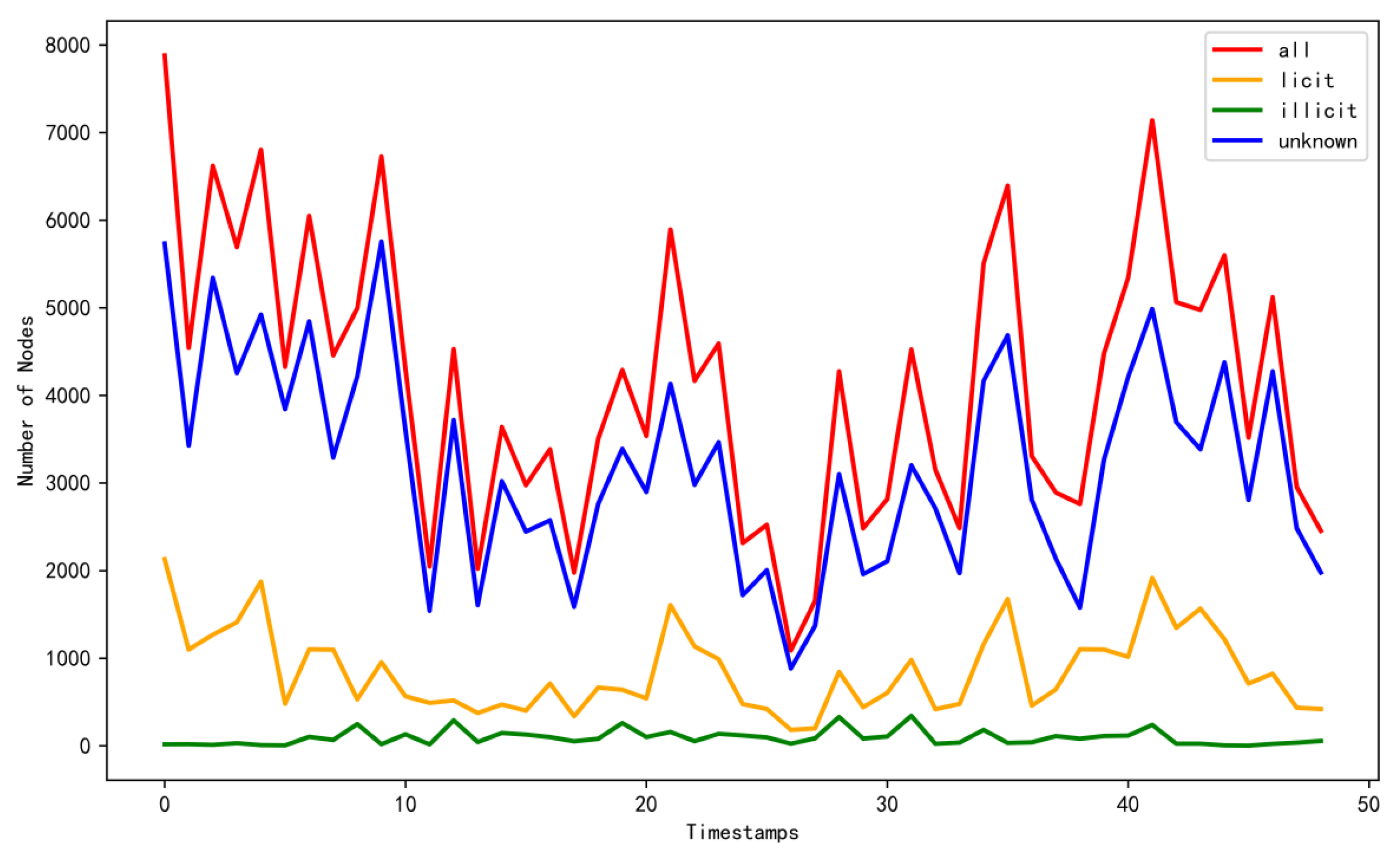
The Elliptic graph dataset is a publicly available Bitcoin transaction dataset associated with illicit money laundering activities that was jointly released by the Elliptic blockchain analytics company and the Massachusetts Institute of Technology (MIT). This dataset documents 203,769 Bitcoin transactions that are worth approximately $6 billion. Among the 203,769 nodes and 234,355 edges, 2% of the nodes were labeled illicit, 21% were labeled licit, and the remaining 77% were unlabeled. In this graph, each node represents a transaction, and the edges denote the flow of Bitcoin between pairs of transactions. Each node is characterized by 166 features, including timestamp information, with timestamp values ranging from 1 to 49. Figure 1 illustrates the variations exhibited by the sample quantities of different categories over time in the Elliptic dataset, with a time interval of approximately two weeks between adjacent timestamps.

To validate the effectiveness and generalizability of the proposed method, given the scarcity and sensitivity of the available financial transaction graph datasets, we select the OGB-Arxiv graph dataset as an additional experimental control group. OGB-Arxiv is an open benchmark graph dataset released by Stanford University in 2019 that contains 169,343 nodes and 1,166,243 edges. In this dataset, nodes represent academic papers, and edges denote citation relationships between papers. Each node is associated with a 128-dimensional feature vector representing the keywords of the corresponding paper and a temporal feature named “year,” indicating the publication year of the paper and ranging from 1979 to 2019. Due to the relatively limited number of data samples before 2006, a data merging process was applied in the experiments to alleviate the excessive parameter fluctuations that occurred at early timestamps. The primary task of the OGB-Arxiv graph dataset is to predict the main categories of Arxiv academic papers, encompassing a total of 40 different classes.

Compared to the Elliptic graph dataset, the OGB-Arxiv graph dataset exhibits similar dynamic node features but possesses more intricate edge relationships and a richer set of categories. Therefore, this dataset is better suited for validating the predictive performance of the method proposed in this study when addressing complex graph datasets.

4.1.2. Evaluation Metric Selection

In the experiments conducted in this paper, a series of evaluation metrics are employed to gauge the performance of the proposed model, including the micro-precision, micro-recall, micro-F1, macro-precision, macro-recall, and macro-F1 values. The computational formulas for these evaluation metrics are outlined in Equation (9):

$$\begin{array}{c}\begin{array}{c}Micro-Precision=\frac{\sum _{i=1}^n{TP}_i}{\sum _{i=1}^n{TP}_i+\sum _{i=1}^n{FP}_i}\\ Micro-Recall=\frac{\sum _{i=1}^n{TP}_i}{\sum _{i=1}^n{TP}_i+\sum _{i=1}^n{FN}_i}\\ Micro-F1=\frac{2 \times Micro - Precision \times Micro - Recall}{Micro - Precision + Micro - Recall}\end{array}\\ \begin{array}{c}Macro-Precision=\frac{1}{n}{\displaystyle \sum _{i=1}^n}{Precision}_i\\ Macro-Recall=\frac{1}{n}{\displaystyle \sum _{i=1}^n}{Recall}_i\\ Macro-F1=\frac{2 \times Macro - Precision \times Macro - Recall}{Macro - Precision + Macro - Recall}\end{array}\end{array}$$

(9)

In the provided formulas, $n$ represents the total number of categories, ${TP}_i$ denotes the number of samples in category $i$ that are correctly predicted as positive, ${FP}_i$ indicates the number of samples in category $i$ that are erroneously predicted as positive, and ${FN}_i$ represents the number of samples in category $i$ that are correctly predicted as negative. ${Precision}_i$ signifies the probability that the samples predicted by the model as positive for category $i$ are indeed positive. ${Recall}_i$ represents the probability that the model correctly predicts the samples that actually belong to the positive class for category $i$.

In this paper, the macro-F1 score is adopted as the primary evaluation metric; this choice is motivated by the highly imbalanced sample distribution in the Elliptic dataset. As depicted in Figure 4, the number of nodes associated with illicit money laundering in the Elliptic dataset is significantly lower than that associated with legitimate nodes. In such a scenario, models tend to achieve better performance on categories with larger sample distributions, while their performance diminishes on categories with fewer samples. Given that our research emphasis lies in predicting illicit money laundering transactions, strong emphasis must be placed on relatively scarce illicit transaction samples.

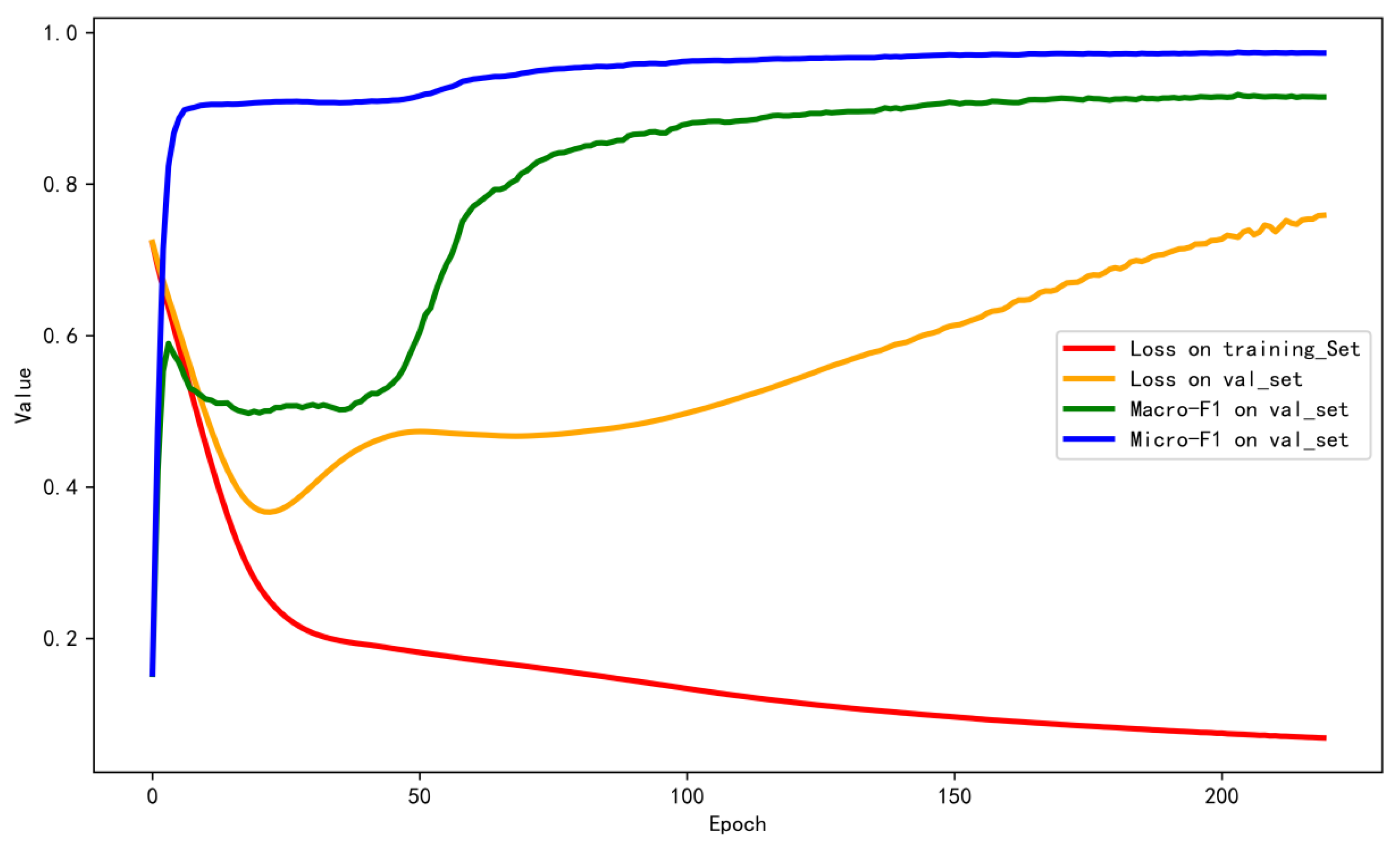
To validate the advantages of employing the macro-F1 score as an evaluation metric, we illustrate the trends exhibited by various evaluation metrics during the model training process across different training epochs in Figure 5. Additionally, Figure 6 shows the variations in each element of the confusion matrix as the number of epochs increases.

As shown in Figure 5, the MDGC-LSTM model induces the lowest loss in the validation set after 25 training epochs, with the micro-F1 score approaching 0.9. The confusion matrix in Figure 6 indicates that at this moment, the predictions produced by the model for legitimate transaction samples are nearly perfect. However, its ability to detect illicit money laundering transactions is quite limited, as reflected by the fact that the true negative (TN) values approach zero.

As the number of training epochs approaches 75, the micro-F1 score stabilizes, while the macro-F1 score continues to gradually increase, which is consistent with the trend exhibited by the TN values in Figure 6. This finding suggests an ongoing improvement in the ability of the model to predict illicit money laundering transactions. These observations underscore the rationale behind using the macro-F1 score as an evaluation metric, particularly when addressing highly imbalanced sample distributions.

4.1.3. Model Parameter Selection

The experiments in this paper build upon prior research findings [30] and incorporate the latest advancements in dynamic graph convolution theory [32]. Consequently, the primary parameter configurations in these experiments align with those used in a preceding study [33]. Message passing and aggregation operations are implemented on the given money laundering transaction graph using the open-source DGL toolkit [46]. Detailed information regarding the experimental parameters is provided in

Table 2. Parameter settings for training the MDGC-LSTM model.

Parameter	Value
Training set proportion	80%
Validation set proportion	10%
Test set proportion	10%
RNN_layers	2
Graph_layers	2
Support	2
Training epochs	220
Lr	0.001
Loss function	Cross entropy
Optimizer	Adam
Weight_decay	5 × 10−5
Activation function	ReLU

.

In contrast with the previous study in [33], we do not employ an early stopping mechanism. This decision is informed by the observed trends in the model evaluation metrics across different training epochs, as depicted in Figure 5. It is evident that the model achieves its minimum loss on the validation set after approximately 25 epochs, while the macro-F1 score begins to stabilize at approximately 150 epochs. Therefore, this study opts not to use an early stopping mechanism and instead maintains a consistent model training process for 220 epochs.

In Table 2, “RNN_layers” denotes the number of layers in RNN models such as LSTM and a GRU, while “Graph_layers” represents the number of layers in the graph convolution model. The “Support” parameter signifies the depth of the node neighborhood during the graph convolution process, where a “Support” value of 2 indicates the adoption of second-order neighborhood nodes for graph convolution purposes. “Lr” represents the initial learning rate of the model. We determine the optimal settings for these two parameters by referencing prior research [33].

During the experimental process, we utilize the cross-entropy loss function to assess the disparity between the model predictions and the actual values. For a multiclass classification problem with N classes, given the true class label y for a particular sample and the model output probability p, the formula for calculating the cross-entropy loss is as follows:

$$\begin{array}{c}L\left(y,P\right)=-{\displaystyle \sum _{i=1}^N}\left(y_i\log P_i\right)\\ P_i=\frac{e^{W_i^T{x}_i+b_i}}{\sum _{j=1}^N{e}^{W_j^T{x}_j+b_j}}\end{array}$$

(10)

Here, $y_i$ represents the true class of the sample, and $P_i$ denotes the probability value predicted by the model for class $i$, i.e., the output of the softmax layer. $W$ represents the classification weights of the fully connected layer, and $b$ represents the bias term.

In the experiments, we employ adaptive moment estimation (Adam) as the optimizer, which is an optimization algorithm that combines momentum and adaptive learning rates, aiding in effectively converging the loss function to its minimum value. Additionally, we utilize the Weight_decay parameter optimization strategy, which is a regularization technique that helps control the complexity of the model and reduce the risk of overfitting. Finally, we apply a rectified linear unit (ReLU) as the activation function, as this method is widely used in deep learning scenarios to introduce nonlinearity and contributes to better capturing the complex relationships within data.

4.1.4. Baselines

To validate the effectiveness of the proposed MDGC-LSTM method in the field of money laundering prediction, we conduct a comprehensive comparison with six traditional machine learning models and six deep learning-based models.

Among the six traditional machine learning models, the first is logistic regression (LR) [16,17], which is a widely used linear model for classification problems that predicts the probabilities of output categories by combining the input features with weights and applying a logistic function. The second is an SVM [18,19], which is a classification and regression model that was designed to find an optimal hyperplane for establishing the maximum margins between data points belonging to different classes. The next model is a random forest (RF) [20], which is an ensemble learning model based on predictions derived from multiple decision trees that achieves enhanced model performance and robustness through voting or averaging. Backpropagation (BP) [21] is a training algorithm for shallow neural networks in which the network weights are updated by backpropagating errors to minimize the discrepancy between the predicted outputs and the actual targets. Additionally, both extreme gradient boosting (XGBoost) [47] and the light gradient boosting machine (LightGBM) [48] are gradient boosting tree models, with XGBoost iteratively training multiple trees to minimize prediction errors and incorporating gradient boosting and regularization techniques to attain improved model performance. LightGBM employs a histogram-based learning algorithm to increase training speed and reduce memory usage, and this method is suitable for large-scale datasets and high-dimensional features.

Among the six deep learning-based models, the GRU [27] and LSTM [24] models are RNN variants used for handling sequential data. They address the vanishing and exploding gradient issues faced by traditional RNNs by introducing gate mechanisms that capture long-term dependencies. Furthermore, a GCN [28] is a deep learning model for processing graph data that captures the relationships between nodes by performing convolution operations on the input graph structure. GCN-GRU and MGC-LSTM [33] are fusion models that execute graph convolution operations on a static graph constructed from the entire training set in combination with GRUs and LSTM networks, respectively. The DGCN-GRU constructs graph snapshots using dynamic data for each timestamp, performs graph convolution operations on these snapshots, and utilizes GRUs to capture sequential properties, enabling complex time series graph data to be comprehensively modeled.

4.2. Experimental Results and Analysis

This section aims to validate the effectiveness of the proposed MDGC-LSTM method in the field of money laundering prediction and examine its performance in terms of handling complex dynamic graph data.

Table 3. Comparison among the prediction results obtained by MDGC-LSTM and other deep learning models on the Elliptic dataset.

Dataset	Model	Micro-Precision	Micro-Recall	Micro-F1	Macro-Precision	Macro-Recall	Macro-F1	Ex-Time(s)
Elliptic	GRU	0.9345	0.9345	0.9345	0.8670	0.6937	0.7474	12.58
	LSTM	0.9364	0.9364	0.9364	0.8651	0.7104	0.7619	14.50
	GCN	0.9192	0.9192	0.9192	0.7596	0.8173	0.7844	14.73
	GCN-GRU	0.9310	0.9310	0.9310	0.7927	0.8103	0.8012	30.50
	MGC-LSTM	0.9351	0.9351	0.9351	0.8107	0.7938	0.8019	32.95
	DGCN-GRU	0.9360	0.9360	0.9360	0.8096	0.8109	0.8103	27.20
	MDGC-LSTM	0.9435	0.9435	0.9435	0.8380	0.8161	0.8266	30.34

and

Table 4. Comparison among the prediction results obtained by MDGC-LSTM and other deep learning models on the OGB-Arxiv dataset.

Dataset	Model	Micro-Precision	Micro-Recall	Micro-F1	Macro-Precision	Macro-Recall	Macro-F1	Ex-Time(s)
OGB- Arxiv	GRU	0.2814	0.2435	0.2331	0.2814	0.2435	0.2331	71.08
	LSTM	0.2747	0.2434	0.2398	0.2747	0.2434	0.2398	92.41
	GCN	0.2992	0.2495	0.2476	0.2992	0.2495	0.2476	94.66
	GCN-GRU	0.3635	0.2589	0.2708	0.3635	0.2589	0.2708	175.69
	MGC-LSTM	0.3536	0.2675	0.2804	0.3536	0.2675	0.2804	209.18
	DGCN-GRU	0.3157	0.3011	0.2988	0.3157	0.3011	0.2988	162.05
	MDGC-LSTM	0.3414	0.3131	0.3169	0.3414	0.3131	0.3169	202.43

provide summaries of the model evaluation results obtained by the baseline deep learning models and the proposed method on the Elliptic and OGB-Arxiv datasets, respectively. Notably, the evaluation results of different models in the tables represent the best performance achieved across all 49 timestamps. Additionally, Figure 7 illustrates the variation trends exhibited by the macro-F1 scores of the different deep learning models at each timestamp during the model training phase.

The experimental results demonstrate the significant advantage of the proposed MDGC-LSTM method in terms of the macro-F1 score. The MDGC-LSTM model cleverly integrates spatial correlation features and temporal feature extraction, leveraging the properties of dynamic graph convolution and LSTM. This integration allows the model to accurately capture complex dynamic patterns within the given dataset, leading to a substantial money laundering prediction advantage over the other comparative methods.

Furthermore, we observe that the macro-recall values of the GRU and LSTM are notably lower than those of the GCN and the other fusion methods, and their macro-F1 values that are also lower than those of the GCN. This may be attributed to the limitations of the methods in terms of handling dynamic graph data. The GCN and the other fusion methods effectively utilize graph convolution operations to better capture the spatial correlation features within each dataset.

A closer examination reveals that the performances of MDGC-LSTM and DGCN-GRU, which use dynamic graph convolution, surpass those of MGC-LSTM and GCN-GRU, which employ static graph convolution. Static graph convolution conducts message passing among nodes based on a graph constructed from the entire set of transaction behaviors, and each timestamp involves message passing among the node features within the graph. As messages are repeatedly passed over multiple timestamps, the features of transaction nodes from earlier timestamps are involved in multiple message passing operations, leading to the gradual smoothing of the node features. This smoothing effect causes reductions in the feature differences among the nodes, making it challenging for the model to distinguish between different nodes, resulting in suboptimal performance in the task of detecting illicit money laundering transactions.

In contrast, dynamic graph convolution better simulates real-world scenarios. In a money laundering prediction task, the transaction behavior at each timestamp is treated as an independent snapshot, and the temporal features that are inherent to each timestamp can be effectively mined. Moreover, as future transaction behaviors cannot be detected at the current timestamp, constructing a static graph based on the entire transaction behavior set is unreasonable in money laundering prediction scenarios and may result in information leakage issues. Therefore, dynamic graph convolution aligns better with the practical application requirements and effectively enhances the performance of the developed model.

Figure 7 shows that the seven different deep learning methods exhibit similar performance trends across all timestamps. At the initial four timestamps, the GCN performs exceptionally well, possibly because as a relatively simple model, the GCN is only used to extract the spatial correlation features of the transaction nodes, resulting in lower model complexity and faster convergence. However, at later timestamps, the proposed MDGC-LSTM approach significantly outperforms the other six methods. This can be attributed to MGDC-LSTM’s utilization of dynamic graph convolution and LSTM for feature extraction in both temporal and spatial dimensions. Compared to single-dimensional models, MGDC-LSTM is better equipped to capture the spatiotemporal correlations present in the dataset. Furthermore, in contrast to static graph convolution, MGDC-LSTM can more effectively extract temporal features of transaction nodes, thereby achieving optimal detection accuracy.

Notably, at timestamp 43, a significant decline is observed in the predictive performance of all the models. This downward trend is attributed to the sudden closure of the world’s largest black market trading network. The shutdown of the black market trading network eliminates instances of illicit transactions from the dataset, rendering the algorithms incapable of capturing the latest features of illicit transactions.

In addition to comparing the proposed approach with different deep learning methods, this study also conducts a comprehensive comparison between MDGC-LSTM and traditional machine learning methods.

Table 5. Comparison among the prediction results obtained by MDGC-LSTM and other machine learning models on the Elliptic dataset.

Dataset	Model	Micro-Precision	Micro-Recall	Micro-F1	Macro-Precision	Macro-Recall	Macro-F1	Ex-Time(s)
Elliptic	LR	0.9338	0.9338	0.9338	0.8356	0.7372	0.7755	0.24
	SVM	0.9540	0.9540	0.9540	0.9758	0.7584	0.8283	4893
	RF	0.9531	0.9531	0.9531	0.9691	0.7558	0.8247	0.34
	BP	0.9596	0.9596	0.9596	0.9231	0.8282	0.8681	3.96
	XGBoost	0.9600	0.9600	0.9600	0.9119	0.8419	0.8728	0.38
	LightGBM	0.9598	0.9598	0.9598	0.9099	0.8428	0.8725	0.45
	MDGC-LSTM	0.9742	0.9742	0.9742	0.9491	0.8922	0.9183	30.34

and

Table 6. Comparison among the prediction results obtained by MDGC-LSTM and other machine learning models on the OGB-Arxiv dataset.

Dataset	Model	Micro-Precision	Micro-Recall	Micro-F1	Macro-Precision	Macro-Recall	Macro-F1	Ex-Time(s)
OGB-Arxiv	LR	0.4102	0.4102	0.4102	0.1344	0.1104	0.0974	1.12
	SVM	0.2759	0.2759	0.2759	0.4013	0.1061	0.1351	26084
	RF	0.2441	0.2441	0.2441	0.1855	0.2575	0.1687	1.77
	BP	0.4425	0.4425	0.4425	0.2814	0.2435	0.2331	21.72
	XGBoost	0.3482	0.3482	0.3482	0.1888	0.1069	0.1095	1.92
	LightGBM	0.2701	0.2701	0.2701	0.2018	0.2824	0.1873	2.61
	MDGC-LSTM	0.5629	0.5629	0.5629	0.4202	0.3486	0.3715	202.43

provide detailed summaries of the model evaluation results obtained by the baseline traditional machine learning models and the proposed method on the Elliptic and OGB-Arxiv datasets, respectively.

Traditional machine learning models, such as SVMs, typically differ from neural networks due to their inability to dynamically load previous model parameters. Their parameters are typically saved in the form of model coefficients and intercepts, making it challenging to attain dynamic predictions. According to the experimental results presented in Table 5 and Table 6, the traditional machine learning models undergo a single training session on the entire training set and are subsequently evaluated on the validation set. This setup results in the macro-F1 values in Table 5 and Table 6 generally exceeding the dynamic temporal prediction results provided in Table 3 and Table 4.

During the experiments, we meticulously tuned the parameters of all the models. The parameters for the LR and RF algorithms are referenced from [33], the parameters for the SVM are referenced from [18], the parameters for the BP algorithm are referenced from [19], the parameters for the XGBoost model are derived from [47], and the parameters for the LightGBM model are acquired from [48]. The results presented in Table 5 and Table 6 clearly indicate that the proposed MDGC-LSTM method can effectively extract spatial and temporal features from each dataset, demonstrating a pronounced advantage over traditional algorithms.

Notably, the performances achieved by the traditional machine learning algorithms on the OGB-Arxiv dataset are noticeably lower than their performances on the Elliptic dataset. This might stem from the fact that the OGB-Arxiv dataset contains a greater number of categories (totaling 40), making its detection task a highly complex multiclass classification problem. Traditional machine learning methods exhibit certain limitations when handling such intricate classification problems, as they struggle to fully unleash their potential performance.

4.3. Model Parameter Comparison and Analysis

4.3.1. Impact of the Graph Convolutional Layer Depth

Figure 8 shows a comparison among the macro-F1 scores produced on the Elliptic validation set by the MDGC-LSTM model with different graph convolutional layer depths.

Figure 8 shows that the MDGC-LSTM model achieves optimal performance when the number of graph convolutional layers is set to 2. As the number of graph convolutional layers increases from 1 to 2, the performance of the model significantly improves. However, with further increases in the number of graph convolutional layers, the performance of the model gradually declines. Therefore, in Table 2, this study sets the parameter representing the number of graph convolutional layers, Graph_layers, to 2.

Excessive graph convolutional layers can lead to oversmoothing, subsequently diminishing the illicit money laundering transaction prediction performance of the model [49]. This is because as the number of graph convolutional layers increases, node features are influenced by more distant nodes, resulting in the averaging of node features. With the increase in the number of layers, the node features gradually become more homogeneous, reducing the feature differences among the nodes. This smoothing effect makes it challenging for the network to distinguish subtle feature differences among the different nodes, thereby diminishing the discrimination ability of the network.

4.3.2. Impact of Graph Convolutional Dropout

Figure 9 shows a performance comparison among various evaluation metrics produced by the MDGC-LSTM model on the Elliptic validation set when employing different dropout coefficients during the graph convolution process.

Figure 9 shows that when the dropout coefficient is set to 0.2, the model achieves its maximum macro-F1 score on the validation set, indicating optimal money laundering transaction prediction performance at this dropout rate. During the training process with dropout introduced in the graph convolution layers, neural network units are temporarily removed from the network with a certain probability. Each graph convolution step involves only message passing and aggregation for a subset of nodes. This approach is equivalent to training the model using a subgraph of the overall transaction graph each time, effectively preventing the model from overfitting on the training set. With an increase in the dropout parameter, the macro-recall value steadily improves, validating the effective reduction in the risk of overfitting through the use of graph convolution dropout.

However, when the dropout coefficient increases to 0.3, although the macro-recall value continues to improve, the validation precision of the model significantly decreases, indicating that excessively high dropout rates lead to difficulty in terms of learning on the training set and result in underfitting. Therefore, considering the macro-F1 evaluation metric of the model, this study sets the dropout coefficient in the graph convolution layers to 0.2.

4.3.3. Impact of the Weight Decay Coefficient

Figure 10 shows a comparison among the macro-F1 values produced on the Elliptic validation set by the MDGC-LSTM model during the training process with different weight decay coefficients.

As a regularization technique, Weight_decay imposes an L2 norm penalty on the model weights within the loss function, restraining the growth of the model weights to reduce the complexity of the model and alleviate overfitting. For the MDGC-LSTM model, with the introduction of the Weight_decay parameter, the weight updating rule is as follows:

$$W_{t+1}=W_t-\gamma \left(\frac{\partial L_0}{\partial W_t}+\lambda W_t\right)$$

(11)

Here, $W_t$ represents the model parameters at update step $t$, $\frac{\partial L_0}{\partial W_t}$ denotes the raw gradient computed from the loss value, $\gamma$ is the learning rate, and $\lambda$ is the Weight_decay coefficient.

Figure 10 shows that the integration of the Weight_decay parameter into the MDGC-LSTM model results in a slight improvement in the macro-precision value, while the macro-recall and macro-F1 values significantly increase. This indicates that without using weight decay, the model exhibits some overfitting tendencies on the training set, and with the incorporation of the Weight_decay parameter, the ability of the model to generalize to new datasets is effectively improved. Therefore, in Table 2, this study sets the Weight_decay parameter to 5 × 10⁻⁵, leading to a noticeable improvement in the money laundering prediction performance of the model.

5. Conclusions

To mitigate the risks posed by money laundering in financial transactions, we propose a money laundering prediction model, MDGC-LSTM, based on deep learning to address the spatiotemporal complexity of money laundering transaction data. By integrating MDGC and LSTM, MDGC-LSTM can accurately capture the multilayer relationships that are present within transaction data. The utilization of spatiotemporal relationship graphs constructed from dynamic graph snapshots enables the model to perform comprehensive feature modeling on both temporal and spatial structures.

While our approach has achieved some success in dealing with money laundering transaction data, the scarcity of such data has limited our ability to validate and refine our methods in more diverse scenarios. Nevertheless, any transaction scenario with clear transaction flows and definable transaction features represents a potential application scenario for our proposed method. Therefore, future research efforts should include exploring more extensive datasets and transaction scenarios to validate and refine our methods, extending their applicability to a wider range of practical applications.

References

- Korejo, M.S.; Rajamanickam, R.; Said, M.H.M. The concept of money laundering: A quest for legal definition. J. Money Laund. Control 2021, 24, 725–736. [Google Scholar] [CrossRef]
- Idowu, A.; Obasan, K.A. Anti-money laundering policy and its effects on bank performance in Nigeria. Bus. Intell. J. 2012, 5, 367–373. [Google Scholar]
- Gomber, P.; Kauffman, R.J.; Parker, C.; Weber, B.W. On the fintech revolution: Interpreting the forces of innovation, disruption, and transformation in financial services. J. Manag. Inf. Syst. 2018, 35, 220–265. [Google Scholar] [CrossRef]
- Awotunde, J.B.; Adeniyi, E.A.; Ogundokun, R.O.; Ayo, F.E. Application of big data with fintech in financial services. In Fintech with Artificial Intelligence, Big Data, and Blockchain; Springer: Singapore, 2021; pp. 107–132. [Google Scholar] [CrossRef]
- Juels, A.; Kosba, A.; Shi, E. The ring of gyges: Using smart contracts for crime. Aries 2015, 40, 54. [Google Scholar]
- Dyntu, V.; Dykyi, O. Cryptocurrency in the system of money laundering. Balt. J. Econ. Stud. 2018, 4, 75–81. [Google Scholar] [CrossRef]
- Bouri, E.; Lau, C.K.M.; Lucey, B.; David, R. Trading volume and the predictability of return and volatility in the cryptocurrency market. Financ. Res. Lett. 2019, 29, 340–346. [Google Scholar] [CrossRef]
- Chen, Z.; Khoa, L.D.V.; Teoh, E.N.; Nazir, A.; Karuppiah, E.K.; Lam, K.S. Machine learning techniques for anti-money laundering (AML) solutions in suspicious transaction detection: A review. Knowl. Inf. Syst. 2018, 57, 245–285. [Google Scholar] [CrossRef]
- Zhamiyeva, R.M.; Sultanbekova, G.B.; Abzalbekova, M.T.; Zhakupov, B.A.; Kozhanov, M.G. The role of financial investigations in combating money laundering. Int. J. Electron. Secur. Digit. Forensics 2022, 14, 188–198. [Google Scholar] [CrossRef]
- Ai, L. “Rule-based but risk-oriented” approach for combating money laundering in Chinese financial sectors. J. Money Laund. Control 2012, 15, 198–209. [Google Scholar] [CrossRef]
- Lokanan, M.E. Data mining for statistical analysis of money laundering transactions. J. Money Laund. Control 2019, 22, 753–763. [Google Scholar] [CrossRef]
- Liu, X.; Zhang, P. A scan statistics based suspicious transactions detection model for anti-money laundering (AML) in financial institutions. In Proceedings of the 2010 International Conference on Multimedia Communications, Hong Kong, China, 7–8 August 2010; pp. 210–213. [Google Scholar] [CrossRef]
- Levchenko, V.; Boyko, A.; Bozhenko, V.; Mynenko, S. Money laundering risk in developing and transitive economies: Analysis of cyclic component of time series. Verslas Teor. Ir Prakt./Bus. Theory Pract. 2019, 20, 492–508. [Google Scholar] [CrossRef]
- Gao, Z.; Ye, M. A framework for data mining-based anti-money laundering research. J. Money Laund. Control 2007, 10, 170–179. [Google Scholar] [CrossRef]
- Xia, P.; Ni, Z.; Zhu, X.; He, Q.; Chen, Q. A novel prediction model based on long short-term memory optimised by dynamic evolutionary glowworm swarm optimisation for money laundering risk. Int. J. Bio-Inspired Comput. 2022, 19, 77–86. [Google Scholar] [CrossRef]
- Weber, M.; Domeniconi, G.; Chen, J.; Weidele, D.K.I.; Bellei, C.; Robinson, T.; Leiserson, C.E. Anti-money laundering in bitcoin: Experimenting with graph convolutional networks for financial forensics. arXiv 2019, arXiv:1908.02591. [Google Scholar] [CrossRef]
- Weber, M.; Chen, J.; Suzumura, T.; Pareja, A.; Ma, T.; Kanezashi, H.; Kaler, T.; Leiserson, C.E.; Schardl, T.B. Scalable graph learning for anti-money laundering: A first look. arXiv 2018, 295, 18–32. [Google Scholar] [CrossRef]
- Pambudi, B.N.; Hidayah, I.; Fauziati, S. Improving money laundering detection using optimized support vector machine. In Proceedings of the 2019 International Seminar on Research of Information Technology and Intelligent Systems (ISRITI), Yogyakarta, Indonesia, 5–6 December 2019; pp. 273–278. [Google Scholar] [CrossRef]
- Chen, M.R.; Chen, B.P.; Zeng, G.Q. An adaptive fractional order BP neural network based on extremal optimization for handwritten digits recognition. Neurocomputing 2020, 391, 260–272. [Google Scholar] [CrossRef]
- Jiang, S.; Fengli, Z. Analysis and Prediction of E-Bank Suspicious Accounts Based on Ensemble Learning Under Imbalance Data. Int. Conf. Comput. Financ. Bus. Anal. 2023, 32, 231–242. [Google Scholar]
- Khokhsarai, H.M.; Shahriari, M.; Rudpashti, F.R.; Jaghargh, S.A.S. Presenting a methodology based on the self-organizing maps and multi-layer neural networks for suspected money laundering events at bank branches. J. New Res. Math. 2022, 8, 83–100. [Google Scholar] [CrossRef]
- Wang, S.; Liu, C.; Gao, X.; Qu, H.; Xu, W. Session-based fraud detection in online e-commerce transactions using recurrent neural networks. In Machine Learning and Knowledge Discovery in Databases (Lecture Notes in Computer Science); Springer: Cham, Switzerland, 2017; pp. 241–252. [Google Scholar] [CrossRef]
- Hochreiter, S.; Schmidhuber, J. Long short-term memory. Neural Comput. 1997, 9, 1735–1780. [Google Scholar] [CrossRef]
- Alghofaili, Y.; Albattah, A.; Rassam, M.A. A financial fraud detection model based on LSTM deep learning technique. J. Appl. Secur. Res. 2020, 15, 498–516. [Google Scholar] [CrossRef]
- Zhang, Y.; Yan, B.; Aasma, M. A novel deep learning framework: Prediction and analysis of financial time series using CEEMD and LSTM. Expert Syst. Appl. 2020, 159, 113609. [Google Scholar] [CrossRef]
- Chung, J.; Gulcehre, C.; Cho, K.H.; Bengio, Y. Empirical evaluation of gated recurrent neural networks on sequence modeling. arXiv 2014, arXiv:1412.3555. [Google Scholar] [CrossRef]
- Luo, S.; Ni, Z.; Zhu, X.; Xia, P.; Wu, H. A novel methanol futures price prediction method based on multicycle CNN-GRU and attention mechanism. Arab. J. Sci. Eng. 2023, 48, 1487–1501. [Google Scholar] [CrossRef]
- Labanca, D.; Primerano, L.; Markland-Montgomery, M.; Polino, M.; Carminati, M.; Zanero, S. Amaretto: An active learning framework for money laundering detection. IEEE Access 2022, 10, 41720–41739. [Google Scholar] [CrossRef]
- Alarab, I.; Prakoonwit, S.; Nacer, M.I. Competence of graph convolutional networks for anti-money laundering in bitcoin blockchain. In Proceedings of the 2020 5th International Conference on Machine Learning Technologies, Beijing, China, 19–21 June 2020; pp. 23–27. [Google Scholar] [CrossRef]
- You, J.; Gomes-Selman, J.M.; Ying, R.; Leskovec, J. Identity-aware Graph Neural Networks. Proc. AAAI Conf. Artif. Intell. 2021, 35, 10737–10745. [Google Scholar] [CrossRef]
- Li, G.; Muller, M.; Qian, G.; Perez, I.C.D.; Abualshour, A.; Thabet, A.K.; Ghanem, B. Deepgcns: Making gcns go as deep as cnns. IEEE Trans. Pattern Anal. Mach. Intell. 2021, 45, 6923–6939. [Google Scholar] [CrossRef]
- Mohan, A.; Karthika, P.V.; Sankar, P.; Manohar, M.; Peter, A. Improving anti-money laundering in bitcoin using evolving graph convolutions and deep neural decision forest. Data Technol. Appl. 2022, 57, 313–329. [Google Scholar] [CrossRef]
- Xia, P.; Ni, Z.; Xiao, H.; Zhu, X.; Peng, P. A novel spatiotemporal prediction approach based on graph convolution neural networks and long short-term memory for money laundering fraud. Arab. J. Sci. Eng. 2022, 47, 1921–1937. [Google Scholar] [CrossRef]
- Alarab, I.; Prakoonwit, S. Graph-based lstm for anti-money laundering: Experimenting temporal graph convolutional network with bitcoin data. Neural Process. Lett. 2023, 55, 689–707. [Google Scholar] [CrossRef]
- Jia, B.; Wang, C.; Zhao, H.; Shi, L. An Entity Linking Algorithm Derived from Graph Convolutional Network and Contextualized Semantic Relevance. Symmetry 2022, 14, 2060. [Google Scholar] [CrossRef]
- Yang, W.; Zhang, J.; Cai, J.; Xu, Z. Relation Selective Graph Convolutional Network for Skeleton-Based Action Recognition. Symmetry 2021, 13, 2275. [Google Scholar] [CrossRef]
- You, J.; Du, T.; Leskovec, J. ROLAND: Graph learning framework for dynamic graphs. In Proceedings of the 28th ACM SIGKDD Conference on Knowledge Discovery and Data Mining, Washington, DC, USA, 14–18 August 2022; pp. 2358–2366. [Google Scholar] [CrossRef]
- Zhu, J.; Li, B.; Zhang, Z.; Zhao, L.; Li, H. High-Order Topology-Enhanced Graph Convolutional Networks for Dynamic Graphs. Symmetry 2022, 14, 2218. [Google Scholar] [CrossRef]
- Vaswani, A.; Shazeer, N.; Parmar, N.; Uszkoreit, J.; Jones, L.; Gomez, A.N.; Kaiser, L.; Polosukhin, I. Attention is all you need. In Proceedings of the 2017 Neural Information Processing Systems, Long Beach, CA, USA, 4–9 December 2017; pp. 5998–6008. [Google Scholar]
- Tatulli, M.P.; Paladini, T.; D’Onghia, M.; Carminati, M.; Zanero, S. HAMLET: A Transformer Based Approach for Money Laundering Detection. In Proceedings of the International Symposium on Cyber Security, Cryptology, and Machine Learning, Beer Sheva, Israel, 29–30 June 2023; pp. 234–250. [Google Scholar]
- Huang, H.; Wang, P.; Zhang, Z.; Zhao, Q. A Spatio-Temporal Attention-Based GCN for Anti-money Laundering Transaction Detection. In International Conference on Advanced Data Mining and Applications; Springer: Cham, Switzerland, 2023; pp. 634–648. [Google Scholar] [CrossRef]
- Peng, H.; Wang, H.; Du, B.; Bhuiyan, M.Z.A.; Ma, H.; Liu, J.; Wang, L.; Yang, Z.; Du, L.; Wang, S.; et al. Spatial temporal incidence dynamic graph neural networks for traffic flow forecasting. Inf. Sci. 2020, 521, 277–290. [Google Scholar] [CrossRef]
- Wang, X.; Ma, Y.; Wang, Y.; Jin, W.; Wang, X.; Tang, J.; Jia, C.; Yu, J. Traffic flow prediction via spatial temporal graph neural network. In Proceedings of the Web Conference 2020, Taipei, Taiwan, 20–24 April 2020; pp. 1082–1092. [Google Scholar] [CrossRef]
- Yu, B.; Yin, H.; Zhu, Z. Spatio-temporal graph convolutional networks: A deep learning framework for traffic forecasting. In Proceedings of the Twenty-Seventh International Joint Conference on Artificial Intelligence, Stockholm, Sweden, 13–19 July 2018; pp. 3634–3640. [Google Scholar] [CrossRef]
- Hu, W.; Fey, M.; Zitnik, M.; Dong, Y.; Ren, H.; Liu, B.; Catasta, M.; Leskovec, J. Open graph benchmark: Datasets for machine learning on graphs. Adv. Neural Inf. Process. Syst. 2020, 33, 22118–22133. [Google Scholar] [CrossRef]
- Wang, M.Y. Deep graph library: Towards efficient and scalable deep learning on graphs. In Proceedings of the ICLR Workshop on Representation Learning on Graphs and Manifolds, New Orleans, LA, USA, 6 May 2019. [Google Scholar]
- Ahmed, A. Anti-money laundering recognition through the gradient boosting classifier. Acad. Account. Financ. Stud. J. 2021, 25, 1–11. [Google Scholar]
- Zhang, Y.; Yu, W.; Li, Z.; Raza, S.; Cao, H. Detecting ethereum Ponzi schemes based on improved LightGBM algorithm. IEEE Trans. Comput. Soc. Syst. 2021, 9, 624–637. [Google Scholar] [CrossRef]
- Chen, D.; Lin, Y.; Li, W.; Li, P.; Zhou, J.; Sun, X. Measuring and relieving the over-smoothing problem for graph neural networks from the topological view. Proc. AAAI Conf. Artif. Intell. 2020, 34, 3438–3445. [Google Scholar] [CrossRef]
Figure 1.
Workflow of MDGC-LSTM Model.
Figure 2.
Model fine-tuning for the dynamic graph convolution operation.
Figure 3.
Structural diagram of the LSTM. The “*” symbol represents the elementwise Hadamard product, and the “+” symbol indicates feature addition.
Figure 4.
Distribution of money laundering transaction nodes across dynamic timestamps.
Figure 5.
Trends exhibited by various evaluation metrics of the model across different training epochs.
Figure 6.
Trends of different elements in the confusion matrix over time.
Figure 7.
Temporal trends exhibited by various deep learning models on the Elliptic dataset across 49 timestamps.
Figure 8.
Comparison among the model performance metrics achieved with different numbers of graph convolutional layers.
Figure 9.
Comparison among the model performance metrics achieved with different graph convolutional dropout coefficients.
Figure 10.
Comparison among the model performance metrics achieved with different weight decay coefficients.