
A Deterministic Calibration Method for the Thermodynamic Model of Gas Turbines

1
School of Energy and Power Engineer, Beihang University, Beijing 102206, China
2
Institute for Aero Engine, Tsinghua University, Beijing 102202, China
3
International Innovation Institute, Beihang University, Hangzhou 310023, China
*
Author to whom correspondence should be addressed.
Symmetry 2024, 16(5), 522; https://doi.org/10.3390/sym16050522
Submission received: 11 March 2024
/
Revised: 18 April 2024
/
Accepted: 24 April 2024
/
Published: 26 April 2024
(This article belongs to the Special Issue Carbon Neutrality and Symmetry in Power Engineering and Engineering Thermophysics)
Abstract
:Performance adaptation is an effective way to improve the accuracy of gas turbine performance models. Although current performance adaptation methods, such as those using genetic algorithms or evolutionary computation to modify component characteristic maps, are useful for finding good solutions, they are essentially searching methods and suffer from long computation time. This paper presents a novel approach that can achieve good performance adaptation with low time complexity and without using any searching method. In this method, the actual component performance parameters are first estimated using engine measurements at different operating conditions. For each operating condition, some scaling factors are introduced and calculated to indicate the difference between the actual and predicted component performance parameters. Afterward, an interpolating algorithm is adopted to synthesize the scaling factors for modifying all major component maps. The adapted component maps are then able to make the engine model match all the gas path measurements and achieve the required accuracy of the engine performance model. The proposed approach has been tested with a model high-bypass turbofan engine using simulated data. The results show that the proposed performance adaptation approach can effectively improve the model’s accuracy. Specifically, the prediction errors can be reduced from about 9% to about 0.6%. In addition, this approach has much less computational complexity compared to other optimization-based counterparts.
1. Introduction
The gas turbine engine, a sophisticated piece of thermal equipment with symmetrical geometry, plays an important role in the aerospace industry [1]. To promote the rapid development of the gas turbine, researchers urgently need a good performance model to replace many real engine tests with numerical simulations, which could make the development process more efficient and economical [2]. Additionally, an accurate performance model is crucial for good gas engine controls, diagnostics, and prognostics [3,4].
Generally, the accuracy of a performance model mainly depends on accurate component characteristic maps. However, it is sometimes difficult to obtain the real component maps of an engine due to many different reasons, such as lacking bench testing, performance degradation, and engine-to-engine variations [5,6,7]. Against this limitation, multiple-point performance adaptation methods have drawn more and more attention in recent years [8]. These methods suggest a tuning of generic component maps to make an engine performance model match all measured performances. Typical published work is briefed as follows.
In the early 1990s, Stamatis et al. introduced an adaptation method that was able to calibrate existing component maps by optimizing scaling factors [9,10]. In 2009, Li et al. used a genetic algorithm method to search for an optimal set of scaling factors [11]. In the following years, such a method was further developed by applying variable scaling factors to achieve a nonlinear multiple-point adaptation [12,13]. In 2014, Alberto and Benini performed map modifications in the neighborhoods of the multiple experimental points [14]. An optimization algorithm was applied to seek optimal sets of perturbations on the map in order to minimize the deviation between experimental and predicted performance. Tsoutsanis et al. introduced a novel map representation and an optimization algorithm for the adaptation [15,16]. By employing elliptic curves to generate compressor maps, they refined gas turbine models with improved accuracy. Recently, Pang et al. proposed a joint adaptation method that added a transient performance adaptation procedure following the steady-state counterpart [17]. After a two-step optimization process, engine models can be calibrated to have more accurate transient performance predictions.
The published work for multiple-point performance adaptations involves complex numerical searching and optimizations. Facing such problems, most researchers prefer to employ metaheuristics, such as genetic algorithms [11,12,13,15,16] and evolutionary computation [17]. The metaheuristics can often find good solutions over a huge set of feasible solutions with less computational effort than other optimization methods and proved to be useful approaches for optimization problems [18,19]. However, some drawbacks exist, such as long computing time when the number of points included in the adaptation is large. In addition, metaheuristics do not guarantee that a globally optimal solution can be found [20]. Many heuristic methods contain stochastic procedures so that the solution found is dependent on the set of random variables generated [21]. Furthermore, it is very tricky to specify the appropriate search domain for the adaptation calculations in practice. Therefore, Li et al. explored a non-heuristic method for performance adaptation problems [22]. The method was applied to an industrial gas turbine engine and demonstrated by the comparison results. However, this approach is only suitable to the design point.
This paper proposes a deterministic approach to deal with the multiple-point performance adaptation of gas turbine engines. At first, engine measurements are employed as input information to estimate actual engine performance by a numerical iterative solution process. Next, we compare that performance with the predicted one (using the model with initial component maps) and summarize the comparison using scaling factors. Finally, an interpolation-based algorithm is developed to determine the overall modification of all major component maps. The proposed approach is applied to a model turbofan engine similar to the General Electric CF6 series. Simulation is carried out to demonstrate the capability of the proposed performance adaptation method. The results, discussions, and conclusions are made accordingly.
Compared to the heuristic methods, the novelty of this approach is that a deterministic calibration procedure replaces the searching algorithms to obtain some scaling factors and thus achieves performance adaptation with high accuracy, low computational complexity, and deterministic results.
The remainder of this paper is organized as follows: Section 2 describes the methodology of the proposed deterministic calibration method. Section 3 details the simulation results to demonstrate the effectiveness of the method. Section 4 discusses the method’s advantages in three aspects. The final section provides a summary of this paper.
2. Methodology
2.1. Representation of Map Shift
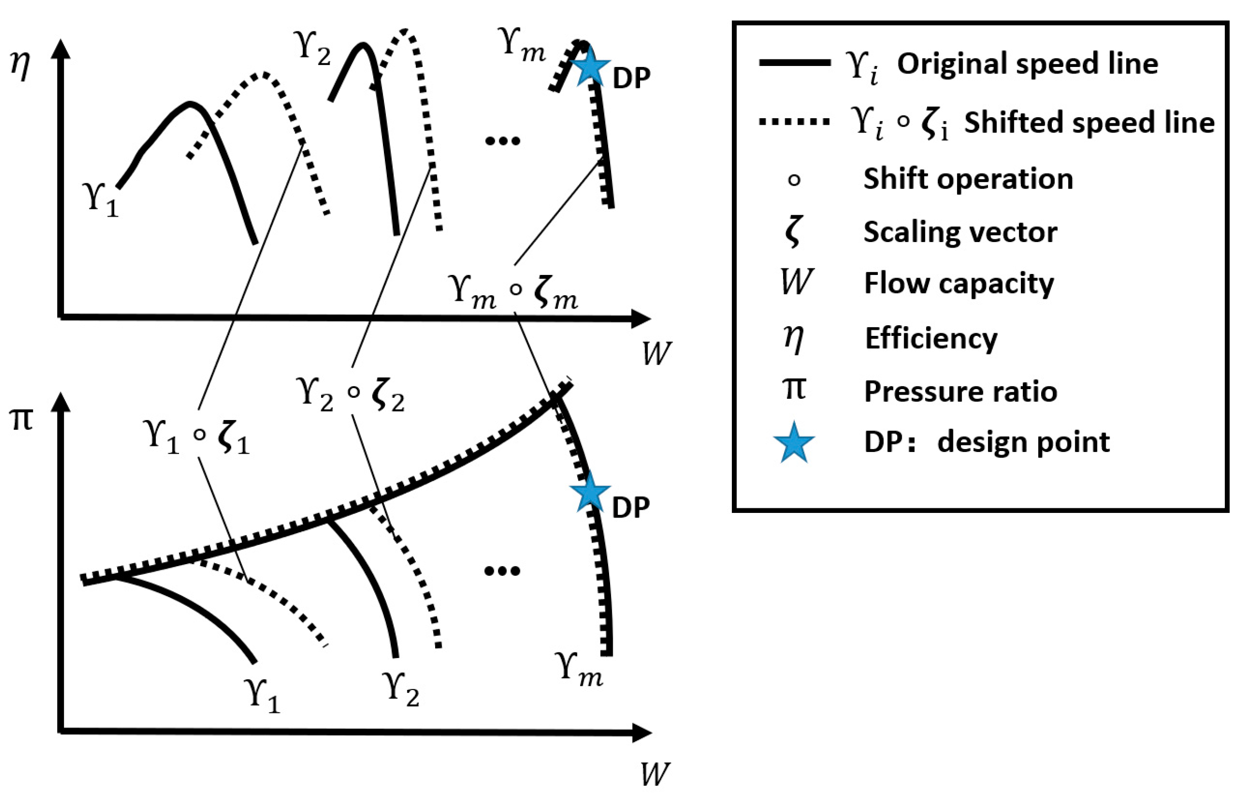
A characteristic map is a chart for describing the performance behavior of an engine component, such as a compressor or a turbine at different operating conditions.
For two major categories of engine components, compressor type, and turbine type, there can be four characteristic parameters to describe the component map: the corrected relative rotational speed n, the flow capacity W, the pressure ratio π, and the isentropic efficiency η. Specifically, a map can be denoted by a group of contour lines (also called the speed lines). Each speed line may be represented by a series of points that have the same speed, n. A map with m (m > 1) speed lines can be defined as
where each is a continuous function from the closed real interval [0,1] into a real coordinate space of 3 dimensions. The speed value of is written as . For a typical high-pressure compressor, for instance, its characteristic map may be illustrated as the solid lines ranging from to in Figure 1.
While the dashed lines in Figure 1 represent a shift of the initial map. For each speed line in the map, an operation ‘’ is defined as Equation (2) to denote its shift.
where means that a speed line is shifted by the vector of scaling factors , where the factors are three real numbers and can be written as a vector for convenience. Then, scaling factor (SF) sets for all speed lines can derive the map shift.
During performance adaptation, the position of the design point (DP) on each component map is assumed to be unchanged. For instance, the DP is located on the mth speed line in Figure 1 and remains unchanged by setting during the entire process of characteristic map shift.
2.2. Scaling Factor Determination
Characteristic maps for compressors and turbines are considered to be adapted in this study. Assume that a map has m speed lines and their speed values are . The objective is to determine their corresponding SF sets .
Assume that measurement data contain M (M ≥ 1) different engine conditions. For each condition, the four characteristic parameters of each concerned component can be estimated by the method described in Section 2.2.1. Afterward, in terms of every single compressor or turbine, SF sets of the M conditions can be determined according to Section 2.2.2. In Section 2.2.3, SF sets are finally obtained by using an interpolation-based algorithm. The above determination process is described in Figure 2.
2.2.1. Actual Performance Estimation
Based on a single-point adaptation method, the performance parameters of all components can be calculated using the given engine measurement data. The single-point adaptation method used in this subsection is developed from existing approaches [22,23] and described as follows.
Owing to the intricate thermodynamic function within the engine system, it is difficult to calculate some performance parameters through measurements directly. However, if guesses of the unknown parameters are introduced, errors can be generated to imply whether the guesses are appropriate by employing the thermodynamic function. Among the errors, the guesses, and the measurements, there exists a relationship that can be represented by Equation (3).
where x is the guess vector of performance parameters, z is the vector of measurement parameters, e is the error vector representing system mismatch between measurement and calculation, and is a differentiable nonlinear function denoting engine thermodynamic function which can generate e from x and z.
Equation (3) is essential for estimating the performance parameters, and it can be obtained by reconstructing the thermodynamic function inside the engine. It contains all the nonlinearities of the complex system.
Remark 1.
e and x should have the same number of elements to avoid Equation (3) underdetermined or overdetermined. By omitting either some less reliable measurements in z or some less important performance parameters in x, the requirement is not difficult to meet.
With given engine measurements z, Equation (3) can be solved by the Newton-Raphson method, which locally linearizes a nonlinear equation at the current estimated value and then uses the linearized equation to update the estimated value to the solution [24]. Iteratively, the error vector e is driven toward zero. And once a converged solution x is obtained, all the other performance parameters, including characteristic parameters of all components, can be predicted.
Remark 2.
The convergence criterion is , where σ is a set threshold.
2.2.2. Scaling Factors at Measured Conditions
Regarding the M measured conditions, this section presents how to determine the SF sets for each component.
At each measured condition, the four characteristic parameters of compressors have been obtained from Section 2.2.1. Figure 3 locates the estimated parameters using a hollow point A.
Normally, point A is not on the corresponding speed line of the existing compressor map. To find the matching point of the current map and the scaling factor between these two points, it is reasonable to assume that the speed line of is shifted along a scaling line where the auxiliary map coordinate is constant [25] to pass through point A. This assumption can locate a solid point B at the intersection of the speed line and the scaling line, as shown in Figure 3. By comparing points A and B, scaling factors can be calculated using Equation (4).
Remark 3.
Although there are three factors in , only two of them are independent because there is a correlation between the scaling factors of corrected flow and that of pressure ratio (under the assumption = constant).
Remark 4.
Note that such a single vector can only reflect the shift at its corresponding speed value . For all M measured conditions whose speed values are , we have to use Equation (4) for M times to obtain the SF sets .
Equation (4) can also be used to determine the scaling factors of turbines. It should be mentioned that the scaling lines with a constant are exactly the same lines with a constant pressure ratio for turbines, as shown in Figure 4. As a result, always holds, i.e., in the turbine case.
2.2.3. Scaling Factors for Map Shifting
For every compressor or turbine, SF sets and their corresponding speed values can be obtained from Section 2.2.2. Meanwhile, speed values of all m initial speed lines are known as . Assume that speed values are written in incremental order, i.e., and .
The following part shows the procedure of how to calculate SFs for each initial map.
- Case 1. M = 1
In the case where there is only one available measured condition, the only scaling vector should be applied to all the speed lines, i.e.,
- Case 2. M > 1
For the case M > 1, if a speed value is located within the interval or next to an endpoint of the interval, it is reasonable to calculate the corresponding scaling vector by using a linear interpolation. In order to represent the range where interpolation can be used, a closed interval, written as “Interval A” in Figure 5, is then defined as where the subscripts “L” and “R” are determined by
and
For each , the corresponding scaling vector can be calculated by Equation (8).
where and
Beyond the range of Interval A, Interval B is further defined (if it exists) where the speed value n is smaller than as shown in Figure 5. Since the interval covers no information on the measured conditions , the nearest scaling vector from Interval A should be applied to all the speed lines in Interval B, i.e.,
Likewise, Interval C is defined (if it exists) and is applied to all the speed lines in it.
So far, all the SFs have been calculated and can be applied to shift the initial characteristic map.
3. Application and Results
3.1. Basic Information of the Model Engine
The proposed multi-point adaptation approach has been applied to a model high-bypass-ratio separate exhaust turbofan engine, commonly used in large passenger and transport aircraft. Among various types of engines, the turbofan engine is the most representative. The configuration of the model (similar to the General Electric CF6 series) is illustrated in Figure 6, with components of intake, fan, booster, high-pressure compressor (HPC), combustor, high-pressure turbine (HPT), low-pressure turbine (LPT), duct and nozzle of bypass, and core. The roles of each component can be referred to [25]. And the number in Figure 6 represents the station of the engine. For example, ‘13′ denotes the outlet of the fan.
The model was created using the Gas Turbine Modeling Library for Education (GTML-E), which was developed on behalf of Beihang University, and an open-source MATLAB/Simulink library for gas turbine performance modeling [26]. The Iterative Newton-Raphson Solver block used in GTML-E is based on the T-MATS package [27].
In this application, five major components are considered to be adapted: the fan, booster, high-pressure compressor, high-pressure turbine, and low-pressure turbine.
For these components, two sets of characteristic maps are prepared separately. The maps in the first set are generic component maps [28] and are regarded as the initial maps. The second set is a transformed version of the first set, where the maps were treated as “real” maps. Note that the “real” maps were only used for generating “test data”.
3.2. “Test Data” Generation
The measurable parameters used in this study are summarized in Table 1, similar to those of CF6 [29]. Some of these parameters are adopted as the model input, while others are regarded as the targeted performance to judge whether the calculated performance is accurate. In the case of validation, except for ambient parameters , only the handle parameter is regarded as the model input. As for the estimation of actual performance, however, more measurable parameters are assumed to be known and used as model inputs.
With the “real” maps applied, “test data” were generated by the model at 10 steady-state operating points under ISA sea-level conditions. These operating conditions of the engine, represented by the handle parameter (normalized fan speed), are listed in Table 2. It can be noticed that 6 of them are employed to carry out the performance adaptation, and all of them are used to demonstrate the effectiveness of this method.
Among the six asterisked conditions, the one with is assumed to be the design point (DP) of the engine. To keep the DP unchanged, this condition has to be chosen as the sticking point for performance adaptation.
3.3. Actual Performance Estimation
For each measured condition, all performance parameters can be estimated by solving Equation (3), where e should converge to zero. At the beginning, all parameters in Equation (3) should be specified. In this case, the parameters in vector z are listed in Table 1. Accordingly, the parameters in x and e are listed in Table 3 and Table 4, respectively.
With all the parameters in Equation (3) specified, the Newton-Raphson method was applied to calculate the true value of the guess parameters. To check whether the final solutions are converged, the infinity norm of every e, as defined in Remark 2, is listed in Table 5. It can be seen that the convergence criterion is satisfied at all six conditions when .
As mentioned in Section 2.2.1, once a converged solution is obtained, the four characteristic parameters for all the concerned components can be calculated.
3.4. Determination of Scaling Factors
For each to-be-adapted component, scaling factor sets at the six measured conditions can be calculated according to Section 2.2.2. Subsequently, SF sets of all the initial speed lines can be determined according to the procedure described in Section 2.2.3 (m represents how many speed lines the initial characteristic map has). Figure 7 plots all the scaling factors of each component, where hollow points denote the result of the six measured conditions, while asterisks represent the result of the initial speed lines whose speed values are . It can be seen that the number of speed lines m varies for different components. For example, m = 12 for the high-pressure compressor while m = 10 for the fan. Additionally, holds for all components referring to the DP points of the components.
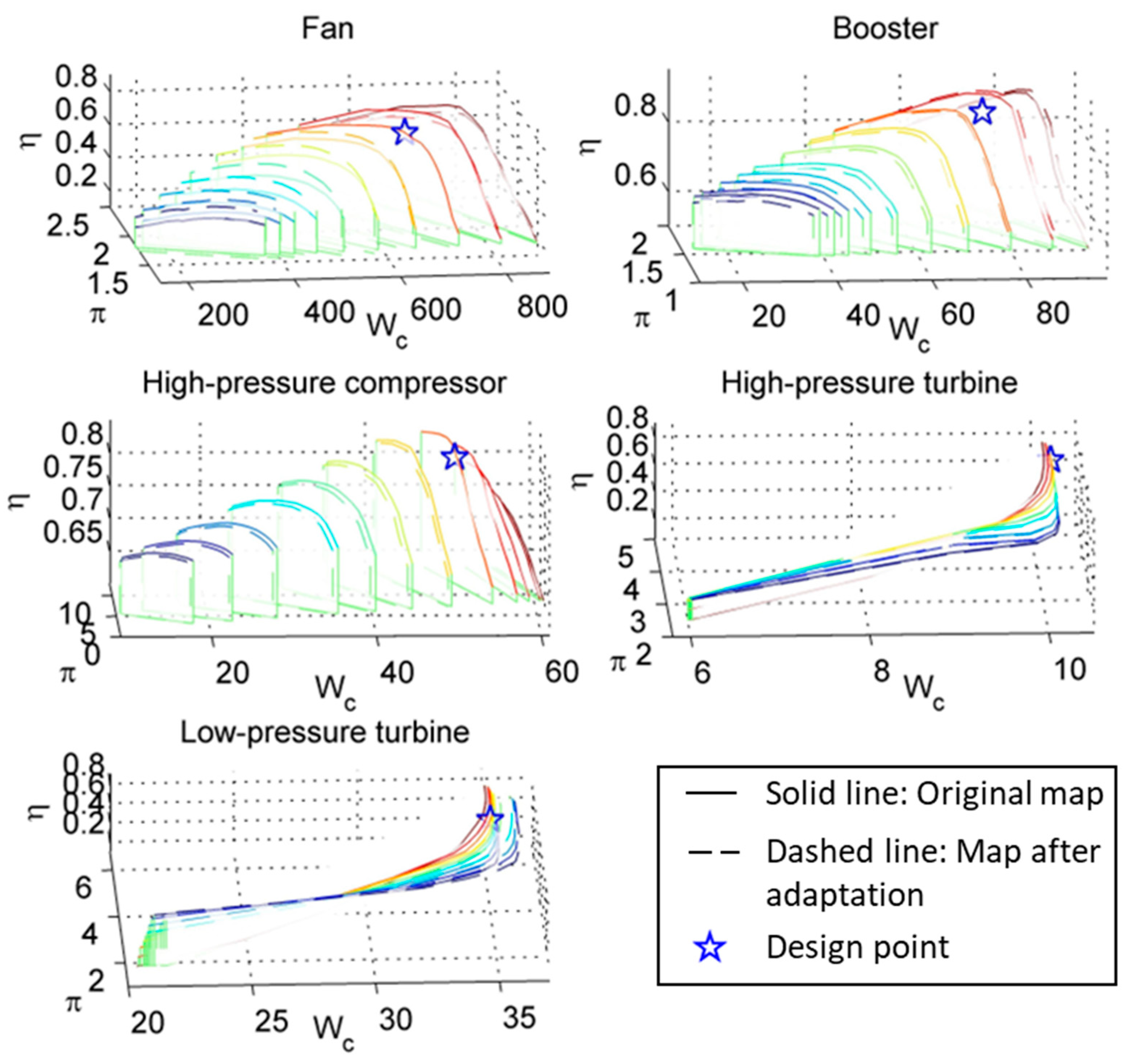
3.5. Adaptation Results
With all the above scaling factors applied to the initial maps, the shifts of the maps are displayed in Figure 8. The solid and dashed curves correspond to the maps before and after the adaptation, respectively. The hollow pentagrams shown in Figure 8 mark the design points whose positions are unchanged during the adaptation.
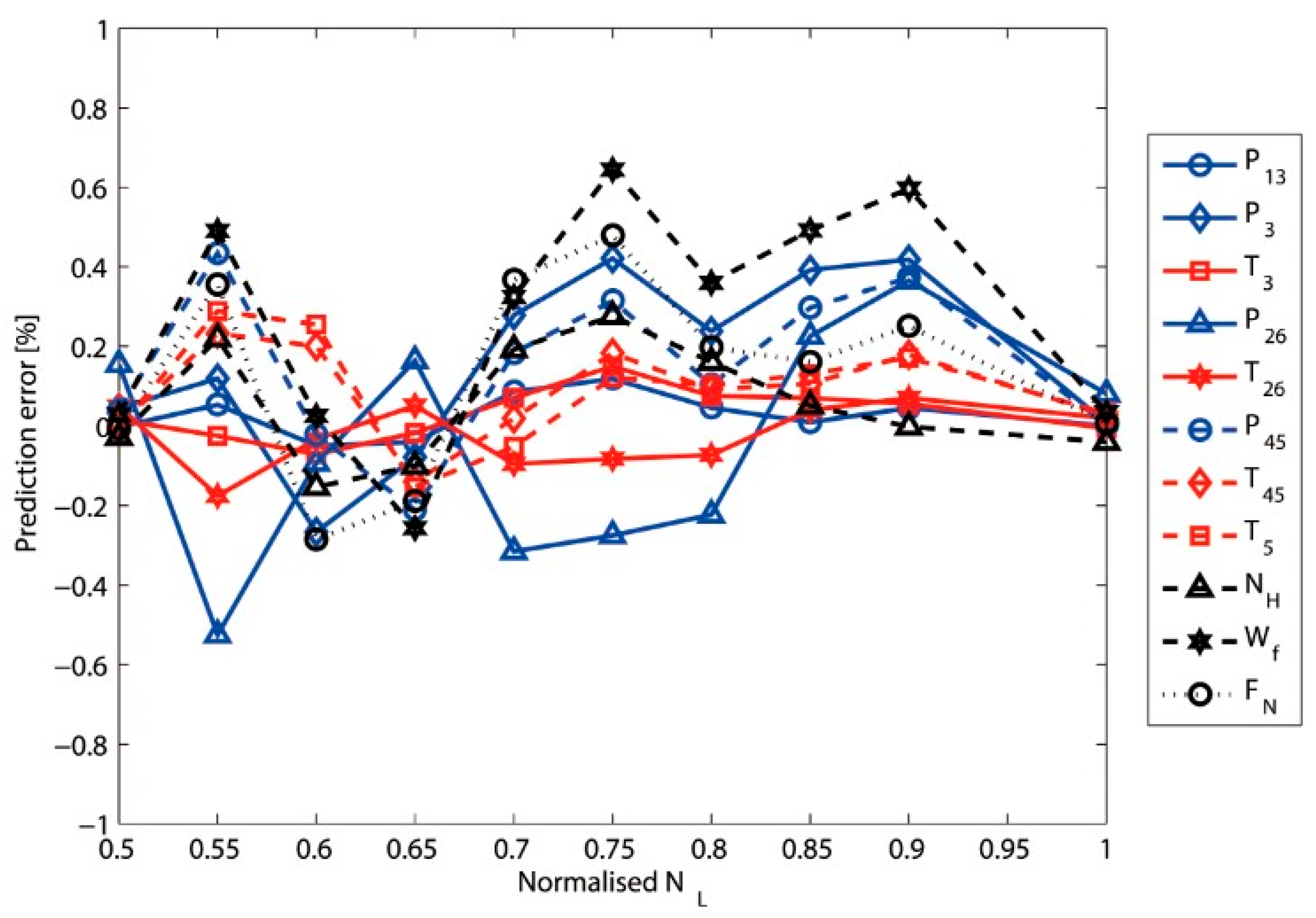
In order to display the effectiveness of the proposed approach, the initial and the adapted characteristic maps are employed to predict the engine performance separately. The prediction errors of the model engine using the initial set of maps covering all 10 conditions are plotted in Figure 9, while the prediction errors of the model engine using the adapted maps are shown in Figure 10. Among all 11 measurable parameters for validation, Figure 9 shows that has a maximum prediction error of about 9% and has a prediction error of about 4%, which greatly affects the accuracy and reliability of the model. While Figure 10 shows the maximum error of about 0.6%, and the prediction error of is significantly reduced to about 0.5%, which indicates good adaptation results. The meaning of these measurable parameters can be acquired in Table 1.
For further validation, five important performance parameters, i.e., bypass ratio BPR, fan pressure ratio , booster pressure ratio , HPC pressure ratio , and turbine temperature ratio , are selected to show the adaption results. The prediction errors before and after the adaptation are plotted in Figure 11 and Figure 12, respectively. It can be seen that these parameters, after adaptation, reach a relatively high level of accuracy, which can support accurate prediction of engine performance.
4. Discussions
4.1. Low Time Complexity
The heuristic approaches for performance adaptation often consume plenty of time. Essentially, heuristic approaches are searching methods that need to try different solutions iteratively until a satisfactory one is found. The time complexity of the approaches mainly depends on how many attempts it takes. Unfortunately, the number of attempts is uncertain because these approaches contain stochastic processes. In practice, both the initial error and the search range may influence the number of attempts. As for the Genetic Algorithm-based adaptation addressed in [6], for example, a four-point adaptation case (20 generations with a population size of 50) took about 50 attempts, i.e., at least 50,000 runs of the model engine. Even though the method was improved by specifying the search range, the number of attempts was still more than 20 (at least 20,000 runs).
Compared to the heuristic approaches, the proposed deterministic approach has quite a lower time complexity. Apart from the actual performance estimation (at most 20 runs for each condition), even there is no need to run the model engine. The computation time of the interpolation algorithm is linearly proportional to the number of speed lines, which is very short and can be ignored in the adaptation process. For a four-point adaptation, the proposed approach needs, at most, 80 runs of the model engine.
4.2. Guaranteed Accuracy
According to Section 2.2.1 and Section 2.2.2, the SF sets at each measured condition can precisely reflect the corresponding measured performance. That is, the accuracy of the model at a particular measured point only depends on measurement accuracy. There is no newly introduced error until the stage to determine SF sets for all the speed lines. At this stage, prediction error will be introduced more or less due to the interpolation algorithm. Fortunately, under the assumption that the component maps and their shifts are smooth enough, the prediction error will be maintained at a relatively low level. In extreme circumstances, we can also add extra speed lines into characteristic maps to improve prediction accuracy. As for the turbofan application, satisfactory accuracy was achieved (max error < 1%) without inserting any extra speed line. Anyway, more accuracy is meaningless for this case because 1% can be covered by measurement uncertainty.
4.3. Sure Solution
Unlike heuristic approaches that have uncertain results, the deterministic approach always has a sure result. As mentioned before, all published approaches for the multi-point adaptation are based on the heuristic algorithm. Using such an algorithm that contains a stochastic process may yield an uncertain solution. As a result, plenty of attempts are required to obtain an acceptable solution, which indeed consumes a great deal of time. Moreover, there is no guarantee that an acceptable solution will be found. In terms of the proposed approach, however, all procedures throughout this paper are deterministic. Consequently, this approach always has a sure solution.
5. Conclusions
This paper presents a deterministic approach for multiple-point performance adaptation, specifically designed to calibrate the off-design performance of gas turbine models. In contrast to the well-developed optimization-based methods, this approach advocates for determining the shift of the initial characteristic maps in a straightforward manner. This concept is realized by calculating each Scaling Factor (SF) set at its corresponding measured condition and subsequently employing an interpolation-based algorithm to ascertain the precise shift of each map.
As discussed in Section 4, this approach offers three primary advantages:
- (1)
- The time complexity of this approach is notably low.
- (2)
- The prediction error of the adapted model can be guaranteed at a relatively low level.
- (3)
- In contrast to optimization-based approaches that entail stochastic procedures, the deterministic approach eliminates the need for a searching procedure and consistently delivers a reliable outcome.
The effectiveness of the proposed approach is demonstrated through its application to a model high-bypass turbofan engine. Following the adaptation process, a significant enhancement in the prediction accuracy of the model is observed, with the prediction error index decreasing from approximately 9% to about 0.6%. Owing to the modification of component maps, the method can be easily transplanted to other engine types and configurations. And with its assured results and minimal computational burden, this approach holds promise as a valuable tool for the calibration of gas turbine models.
The limitation of the proposed deterministic approach is that it is currently suitable for steady-state performance adaptation. The related dynamic performance adaptation and transient analysis need further research. Additionally, only simulated data are used in this paper to illustrate the effectiveness of the method. Applying real engine measurements for verification will be considered in future research. What is more, the impact of measurement uncertainties on model predictions is a direction worth exploring. Uncertainty analysis techniques such as Monto Carlo simulations are an optional solution for conducting future research.
Author Contributions
Conceptualization, Z.J. and S.Y.; methodology, Z.J. and S.Y.; software, S.Y.; validation, M.Z.; formal analysis, X.W.; investigation, Z.J.; resources, S.Y.; data curation, Z.J. and S.Y.; writing—original draft preparation, Z.J. and S.Y.; writing—review and editing, X.W. and M.Z.; visualization, Z.J. and M.Z.; supervision, X.W.; project administration, X.W. and S.Y. All authors have read and agreed to the published version of the manuscript.
Funding
This research received no external funding.
Data Availability Statement
The data that support the findings of this study are available from the corresponding author upon reasonable request.
Conflicts of Interest
The authors declare no conflicts of interest.
Nomenclature
| DP | design point |
| GTML-E | Gas Turbine Modeling Library for Education |
| HPC | high-pressure compressor |
| HPT | high-pressure turbine |
| LPT | low-pressure turbine |
| SF | scaling factor |
| n | corrected relative rotational speed |
| W | flow capacity |
| pressure ratio | |
| isentropic efficiency | |
| contour line of the rotational speed | |
| scaling factor of flow capacity | |
| scaling factor of pressure ratio | |
| scaling factor of isentropic efficiency | |
| vector of the above three scaling factors | |
| speed value at measured conditions | |
| scaling vector at measured conditions |
References
- Miao, K.; Wang, X.; Zhu, M.; Yang, S.; Pei, X.; Jiang, Z. Transient Controller Design Based on Reinforcement Learning for a Turbofan Engine with Actuator Dynamics. Symmetry 2022, 14, 684. [Google Scholar] [CrossRef]
- Cao, J. Status, Challenges and Perspectives of Aero-Engine Simulation Technology. J. Propuls. Technol. 2018, 39, 961–970. [Google Scholar]
- Hanachi, H.; Mechefske, C.; Liu, J.; Banerjee, A.; Chen, Y. Performance-based gas turbine health monitoring, diagnostics, and prognostics: A survey. IEEE Trans. Reliab. 2018, 67, 1340–1363. [Google Scholar] [CrossRef]
- Jiang, Z.; Yang, S.; Wang, X.; Long, Y. An Onboard Adaptive Model for Aero-Engine Performance Fast Estimation. Aerospace 2022, 9, 845. [Google Scholar] [CrossRef]
- Mamala, J.J.; Praznowski, K.; Kołodziej, S.; Ligus, G. The Use of Short-Term Compressed Air Supercharging in a Combustion Engine with Spark Ignition. Int. J. Automot. Mech. Eng. 2021, 18, 8704–8713. [Google Scholar] [CrossRef]
- Cruz-Manzo, S.; Panov, V.; Zhang, Y. Gas path fault and degradation modelling in twin-shaft gas turbines. Machines 2018, 6, 43. [Google Scholar] [CrossRef]
- Panov, V. Auto-tuning of real-time dynamic gas turbine models. Turbo Expo: Power for Land, Sea, and Air. In Proceedings of the ASME Turbo Expo 2014: Turbine Technical Conference and Exposition (GT2014-25606, V006T06A004), Düsseldorf, Germany, 16–20 June 2014. [Google Scholar]
- Hayes, R.; Dwight, R.; Marques, S. Reducing parametric uncertainty in limit-cycle oscillation computational models. Aeronaut. J. 2017, 121, 940–969. [Google Scholar] [CrossRef]
- Stamatis, A.; Mathioudakis, K.; Papailiou, K.D. Adaptive Simulation of Gas Turbine Performance. J. Eng. Gas Turbines Power 1990, 112, 168. [Google Scholar] [CrossRef]
- Lambiris, B.; Mathioudakis, K.; Stamatis, A.; Papailiou, K. Adaptive modeling of jet engine performance with application to condition monitoring. J. Propuls. Power 1994, 10, 890–896. [Google Scholar] [CrossRef]
- Li, Y.G.; Marinai, L.; Gatto, E.L.; Pachidis, V.; Philidis, P. Multiple-point adaptive performance simulation tuned to aeroengine test-bed data. J. Propuls. Power 2009, 25, 635–641. [Google Scholar] [CrossRef]
- Li, Y.G.; Ghafir, M.A.; Wang, L.; Singh, R.; Huang, K.; Feng, X. Nonlinear Multiple Points Gas Turbine Off-Design Performance Adaptation Using a Genetic Algorithm. J. Eng. Gas Turbines Power 2011, 133, 42–50. [Google Scholar] [CrossRef]
- Li, Y.G.; Abdul Ghafir, M.F.; Wang, L.; Singh, R.; Huang, K.; Feng, X.; Zhang, W. Improved Multiple Point Nonlinear Genetic Algorithm Based Performance Adaptation Using Least Square Method. J. Eng. Gas Turbines Power 2012, 134, 031701. [Google Scholar] [CrossRef]
- Alberto Misté, G.; Benini, E. Turbojet engine performance tuning with a new map adaptation concept. J. Eng. Gas Turbines Power 2014, 136, 071202. [Google Scholar] [CrossRef]
- Tsoutsanis, E.; Li, Y.-G.; Pilidis, P.; Newby, M. Non-linear model calibration for off-design performance prediction of gas turbines with experimental data. Aeronaut. J. 2017, 121, 1758–1777. [Google Scholar] [CrossRef]
- Tsoutsanis, E.; Meskin, N.; Benammar, M.; Khorasani, K. A component map tuning method for performance prediction and diagnostics of gas turbine compressors. Appl. Energy 2014, 135, 572–585. [Google Scholar] [CrossRef]
- Pang, S.; Li, Q.; Feng, H.; Zhang, H. Joint steady state and transient performance adaptation for aero engine mathematical model. IEEE Access 2019, 7, 36772–36787. [Google Scholar] [CrossRef]
- Baklacioglu, T.; Turan, O.; Aydin, H. Dynamic modeling of exergy efficiency of turboprop engine components using hybrid genetic algorithm-artificial neural networks. Energy 2015, 86, 709–721. [Google Scholar] [CrossRef]
- Dinc, A. Optimization of a Turboprop UAV for Maximum Loiter and Specific Power Using Genetic Algorithm. Int. J. Turbo Jet-Engines 2016, 33, 265–273. [Google Scholar] [CrossRef]
- Gendreau, M.; Potvin, J.Y. Metaheuristics in combinatorial optimization. Ann. Oper. Res. 2005, 140, 189–213. [Google Scholar] [CrossRef]
- Bianchi, L.; Dorigo, M.; Gambardella, L.M.; Gutjahr, W.J. A survey on metaheuristics for stochastic combinatorial optimization. Nat. Comput. 2009, 8, 239–287. [Google Scholar] [CrossRef]
- Li, Y.G.; Pilidis, P.; Newby, M.A. An adaptation approach for gas turbine design-point performance simulation. J. Eng. Gas Turbines Power 2006, 128, 789–795. [Google Scholar] [CrossRef]
- Roth, B.; Doel, D.L.; Mavris, D.N.; Beeson, D. High-accuracy matching of engine performance models to test data. In Proceedings of the ASME Turbo Expo 2003: Power for Land, Sea and Air (GT2003-38784), Atlanta, GA, USA, 16–19 June 2003; pp. 129–137. [Google Scholar]
- Ortega, J.M.; Rheinboldt, W.C. Iterative Solution of Nonlinear Equations in Several Variables. Math. Comput. 1970, 25, 398. [Google Scholar]
- Kurzke, J.; Halliwell, I. Propulsion and Power: An Exploration of Gas Turbine Performance Modeling; Springer International Publishing: Cham, Switzerland, 2018. [Google Scholar]
- Yang, S. GTML-E: Gas Turbine Modeling Library for Education. 2019. Available online: https://github.com/xjysb/GTML_E (accessed on 1 January 2024).
- Chapman, J.W.; Lavelle, T.M.; May, R.; Litt, J.S.; Guo, T.-H. Propulsion System Simulation Using the Toolbox for the Modeling and Analysis of Thermodynamic Systems (T MATS). In Proceedings of the 50th AIAA/ASME/SAE/ASEE Joint Propulsion Conference (AIAA 2014-3929), Cleveland, OH, USA, 28–30 July 2014; pp. 1–14. [Google Scholar]
- Visser, W.P.; Broomhead, M.J. GSP, a Generic Object-Oriented Gas Turbine Simulation Environment. In Proceedings of the ASME Turbo Expo 2000: Power for Land, Sea, and Air Turbo (V001T01A002), Munich, Germany, 8–11 May 2000. [Google Scholar]
- Dyson, R.J.; Doel, D.L. CF6-80 condition monitoring-the engine manufacturer’s involvement in data acquisition and analysis. In Proceedings of the 20th AIAA//SAE/ASEE Joint Propulsion Conference, Cincinnati, OH, USA, 11–13 June 1984. [Google Scholar] [CrossRef]
Figure 1.
Shift of a compressor map.

Figure 2.
Scaling factor determination process.

Figure 3.
Determine SFs at a measured condition on a compressor map.

Figure 4.
Determine SFs at a measured condition on a turbine map.

Figure 5.
Interval A: the range where interpolation can be used.

Figure 6.
Model turbofan engine configuration.

Figure 7.
Scaling factors of all concerned components.

Figure 8.
Map shift of all concerned components.

Figure 9.
Prediction error of measurable parameters before the adaptation.

Figure 10.
Prediction error of measurable parameters after the adaptation.

Figure 11.
Prediction error of performance parameters before the adaptation.

Figure 12.
Prediction error of performance parameters after the adaptation.


Table 1.
CF6-80 measurable parameters.
| Measurements | Symbol | For Estimation | For Validation |
|---|---|---|---|
| Ambient Pressure | Input | Input | |
| Fan Inlet Temperature | Input | Input | |
| Fan Inlet Pressure | Input | Input | |
| Fuel Flow | Input | Target | |
| Fan Speed | Input | Input | |
| Core Speed | Input | Target | |
| HPC Inlet Temperature | Target | Target | |
| HPC Inlet Pressure | Target | Target | |
| HPC Outlet Temperature | Target | Target | |
| HPC Outlet Pressure | Target | Target | |
| LPT Inlet Temperature | Target | Target | |
| LPT Inlet Pressure | Target | Target | |
| LPT Outlet Temperature | Target | Target | |
| Fan Outlet Pressure | Target | Target | |
| Net Thrust | Input | Target |
Table 2.
Chosen conditions for generating “test data” conditions with asterisks are used for adaptation.
Table 2.
Chosen conditions for generating “test data” conditions with asterisks are used for adaptation.
| No. | No. | ||
|---|---|---|---|
| 1 * | 0.5 | 6 | 0.75 |
| 2 | 0.55 | 7 * | 0.8 |
| 3 * | 0.6 | 8 | 0.85 |
| 4 | 0.65 | 9 * | 0.9 |
| 5 * | 0.7 | 10 * | 1 |
Table 3.
Selected guess parameters.
| No. | Guess | Symbol |
|---|---|---|
| 1 | Fan pressure ratio | |
| 2 | Fan isentropic efficiency | |
| 3 | Booster pressure ratio | |
| 4 | Booster isentropic efficiency | |
| 5 | HPC pressure ratio | |
| 6 | HPC isentropic efficiency | |
| 7 | HPT pressure ratio | |
| 8 | HPT efficiency | |
| 9 | LPT pressure ratio | |
| 10 | LPT efficiency | |
| 11 | Total air flow | |
| 12 | Bypass ratio |
Table 4.
Selected error parameters.
| No. | Error | Symbol |
|---|---|---|
| 1 | Prediction error of | |
| 2 | Flow imbalance in duct nozzle | |
| 3 | Prediction error of | |
| 4 | Prediction error of | |
| 5 | Prediction error of | |
| 6 | Prediction error of | |
| 7 | Prediction error of | |
| 8 | Prediction error of | |
| 9 | Flow imbalance in core nozzle | |
| 10 | Prediction error of | |
| 11 | Torque imbalance of HP spool | |
| 12 | Torque imbalance of LP spool |
Table 5.
Convergence check.
| i | i | ||
|---|---|---|---|
| 1 | 4 | ||
| 2 | 5 | ||
| 3 | 6 |
Disclaimer/Publisher’s Note: The statements, opinions and data contained in all publications are solely those of the individual author(s) and contributor(s) and not of MDPI and/or the editor(s). MDPI and/or the editor(s) disclaim responsibility for any injury to people or property resulting from any ideas, methods, instructions or products referred to in the content. |
© 2024 by the authors. Licensee MDPI, Basel, Switzerland. This article is an open access article distributed under the terms and conditions of the Creative Commons Attribution (CC BY) license (https://creativecommons.org/licenses/by/4.0/).
Share and Cite
MDPI and ACS Style
Jiang, Z.; Wang, X.; Yang, S.; Zhu, M. A Deterministic Calibration Method for the Thermodynamic Model of Gas Turbines. Symmetry 2024, 16, 522. https://doi.org/10.3390/sym16050522
AMA Style
Jiang Z, Wang X, Yang S, Zhu M. A Deterministic Calibration Method for the Thermodynamic Model of Gas Turbines. Symmetry. 2024; 16(5):522. https://doi.org/10.3390/sym16050522
Chicago/Turabian StyleJiang, Zhen, Xi Wang, Shubo Yang, and Meiyin Zhu. 2024. "A Deterministic Calibration Method for the Thermodynamic Model of Gas Turbines" Symmetry 16, no. 5: 522. https://doi.org/10.3390/sym16050522
Note that from the first issue of 2016, this journal uses article numbers instead of page numbers. See further details here.