The Symmetry Group of the Non-Isothermal Navier–Stokes Equations and Turbulence Modelling

Abstract

In this work, the non-isothermal Navier–Stokes equations are studied from the group theory point of view. The symmetry group of the equations is presented and discussed. Some standard turbulence models are analyzed with the symmetries of the equations. A class of turbulence models which preserve the physical properties contained in the symmetry group is built. The proposed turbulence models are applied to an illustrative example of natural convection in a differentially heated cavity, and the results are presented.

1. Introduction

In spite of many decades of studies, turbulence modelling still constitutes an important challenge in engineering science. Indeed, no turbulence model, either with RANS method or with large-eddy simulation (LES) approach, is really satisfying regarding their mathematical and physical properties.

Symmetry preservation is one of the most important properties that a turbulence model should own, since the symmetry group traduces mathematically the physical properties of the flow. Nœther’s theorem [1,2] states indeed that, for a Lagrangian system, each symmetry of the equation corresponds to a conservation law. For example, a system having a time-translation symmetry is energy conserving. In fluid mechanics, the symmetry theory permitted Oberlack to deduce scaling laws, such as algebraic, logarithmic (wall) or exponential laws [3], which have been validated with DNS data [4]. The symmetry approach has also been used to study the dynamics of vortices [5], or to investigate spectral properties of the flow [6].

Speziale was one of the first who tried to include symmetry considerations in turbulence modelling. After examining existing models [7,8], he proposed a general form of Galilean invariant and 2D-material indifferent models. This was followed by the work of Fureby and Tabor [9] and by a discussion with Wang [10,11].

Galilean invariance and 2D-material indifference are only two of the symmetries of the Navier–Stokes equations. Indeed, these equations own other symmetries (see for example [12]), and namely scale invariances which are of particular importance for the establishment of scaling laws for example. However, as pointed out by Oberlack [13], only few turbulence models are consistent with the symmetry group of the Navier–Stokes equations. From this observation, Razafindralandy and Hamdouni proposed a way of building models which preserve the physical properties of a flow contained in the symmetry group [14,15], in the isothermal case. It has been also shown in [15] that the symmetry approach may lead to numerically satisfying models which provide better results than the Smagorinsky and the dynamic models.

This paper aims to extend the work done in [15] to the case of non-isothermal flows. Indeed, for these flows, the subgrid heat flux model is, most of the time, simply deduced from the subgrid stress tensor model by a Reynolds analogy. This analogy limits the scope of the models for strongly coupled problems (natural convection, mixed convection). In this paper, we propose to construct a general class of subgrid stress and heat flux models based on the preservation of the symmetry group (and then the underlying physical properties) of the non-isothermal Navier–Stokes equations (1). More precisely, these models are built such that the LES equations (30) admit the symmetries of the initial equations (1). Next, to reduce the number of arbitrary functions in the class, we impose to the model to derive from a convex potential. This condition guarantees the stability of the model.

This article is organized as follows. A brief introduction to the symmetry group theory is done in Section 2. The Lie point symmetries of the Navier–Stokes equations for non-isothermal flows are then presented. In Section 3., some popular LES models are analyzed with these symmetries. Section 4. is devoted to the construction of the class of models from the symmetry approach. This class is refined in Section 5. using the potential consideration. Some examples of simple models which can easily be integrated into a code for numerical resolution are then deduced. One of these simple models is numerically implemented in Section 6.

2. The Symmetry Group of the Equations

Consider the Navier–Stokes equations for an incompressible, non-isothermal Newtonian fluid, with kinematic viscosity $\nu$ and thermal diffusivity $\kappa$:

$$\left\{\begin{array}{l}\frac{\partial \mathit{u}}{\partial t}+div(\mathit{u}\otimes \mathit{u})+\frac{1}{\rho }\nabla p-div{\tau }_r-\beta g\theta {\mathit{e}}_3=0\hfill \\ \frac{\partial \theta }{\partial t}+div(\theta \mathit{u})-div{\mathbf{h}}_r=0\hfill \\ div\mathit{u}=0\hfill \end{array}\right.$$

(1)

In these expressions,

$${\tau }_r=2\nu \mathsf{S}\mathrm{and}{\mathbf{h}}_r=\kappa \nabla \theta$$

are respectively the viscous stress tensor and the heat flux. The tensor

$$\mathsf{S}=\frac{\nabla \mathit{u}{+}^T\nabla \mathit{u}}{2}$$

is the strain rate tensor. $\beta$ is the thermal expansion and g the acceleration due to gravity. To simplify, we also designate equations (1) by

$$E(\mathbf{q})=0\mathrm{with}\mathbf{q}=(t,\mathit{x},\mathit{u},p,\theta )$$

(2)

In this paper, we consider multiparameter, one point transformations of the form

$$T_a:\mathbf{q}=(t,\mathit{x},\mathit{u},p,\theta )⟼\widehat{\mathbf{q}}=(\widehat{t},\widehat{\mathit{x}},\widehat{\mathit{u}},\widehat{p},\widehat{\theta })$$

(3)

where $\widehat{\mathbf{q}}=\widehat{\mathbf{q}}(\mathbf{q},a)$ depends continuously on the real, eventually local, parameter a. We assume that the parametrization is such that $a=0$ corresponds to the identity. Transformation (3) is a said a symmetry of (1) if it maps each solution of (1) to another solution, i.e.,

$$E(\mathbf{q})=0⟹E(\widehat{\mathbf{q}})=0$$

(4)

The set of the multi-parameter symmetries of (1) constitutes a local Lie group G called the symmetry group of (1). G is characterized by its variation at the vicinity of $a=0$ which is represented by the vector field or infinitesimal generator

$$\mathbf{X}={\eta }_t\frac{\partial }{\partial t}+{\eta }_x\frac{\partial }{\partial x}+{\eta }_y\frac{\partial }{\partial y}+{\eta }_z\frac{\partial }{\partial z}+{\eta }_u\frac{\partial }{\partial u}+{\eta }_v\frac{\partial }{\partial v}+{\eta }_w\frac{\partial }{\partial w}+{\eta }_p\frac{\partial }{\partial p}+{\eta }_{\theta }\frac{\partial }{\partial \theta }$$

(5)

where

$${\eta }_q={\left.\frac{\mathbf{d}\widehat{q}}{\mathbf{d}a}\right|}_{a=0}$$

(6)

Knowing the ${\eta }_q$’s, the expression of $\widehat{\mathbf{q}}$ can be obtained by solving the system

$$\left\{\begin{array}{c}\frac{\mathbf{d}\widehat{\mathbf{q}}}{\mathbf{d}a}={\eta }_q(\widehat{\mathbf{q}})\hfill \\ \widehat{\mathbf{q}}(\mathbf{q},a=0)=\mathbf{q}\hfill \end{array}\right.$$

(7)

For locally integrable equations, Lie’s theory (see [2,16]) permits to replace the symmetry condition (4) by the following one which provides an algorithmic way to compute all the Lie point symmetries of the equations:

$${\mathbf{X}}^{(2)}.E=0\mathrm{when}E(\mathbf{q})=0$$

(8)

${\mathbf{X}}^{(2)}$ is a prolongation of the vector field $\mathbf{X}$, defined in (5), which takes into account the derivative terms in E up to the second order. More precisely,

$$\begin{array}{cc}{\mathbf{X}}^{(2)}=\mathbf{X}\hfill & +{\eta }_u^t\frac{\partial }{\partial u_t}+{\eta }_u^x\frac{\partial }{\partial u_x}+{\eta }_u^y\frac{\partial }{\partial u_y}+{\eta }_u^z\frac{\partial }{\partial u_z}+{\eta }_u^{xx}\frac{\partial }{\partial u_{xx}}+{\eta }_u^{yy}\frac{\partial }{\partial u_{yy}}+{\eta }_u^{zz}\frac{\partial }{\partial u_{zz}}\hfill \\ & +{\eta }_v^t\frac{\partial }{\partial v_t}+{\eta }_v^x\frac{\partial }{\partial v_x}+{\eta }_v^y\frac{\partial }{\partial v_y}+{\eta }_v^z\frac{\partial }{\partial v_z}+{\eta }_v^{xx}\frac{\partial }{\partial v_{xx}}+{\eta }_v^{yy}\frac{\partial }{\partial v_{yy}}+{\eta }_v^{zz}\frac{\partial }{\partial v_{zz}}\hfill \\ & +{\eta }_w^t\frac{\partial }{\partial w_t}+{\eta }_w^x\frac{\partial }{\partial w_x}+{\eta }_w^y\frac{\partial }{\partial w_y}+{\eta }_w^z\frac{\partial }{\partial w_z}+{\eta }_w^{xx}\frac{\partial }{\partial w_{xx}}+{\eta }_w^{yy}\frac{\partial }{\partial w_{yy}}+{\eta }_w^{zz}\frac{\partial }{\partial w_{zz}}\hfill \\ & +{\eta }_p^t\frac{\partial }{\partial p_t}+{\eta }_p^x\frac{\partial }{\partial p_x}+{\eta }_p^y\frac{\partial }{\partial p_y}+{\eta }_p^z\frac{\partial }{\partial p_z}\hfill \\ & +{\eta }_{\theta }^t\frac{\partial }{\partial {\theta }_t}+{\eta }_{\theta }^x\frac{\partial }{\partial {\theta }_x}+{\eta }_{\theta }^y\frac{\partial }{\partial {\theta }_y}+{\eta }_{\theta }^z\frac{\partial }{\partial {\theta }_z}+{\eta }_{\theta }^{xx}\frac{\partial }{\partial {\theta }_{xx}}+{\eta }_{\theta }^{yy}\frac{\partial }{\partial {\theta }_{yy}}+{\eta }_{\theta }^{zz}\frac{\partial }{\partial {\theta }_{zz}}\hfill \end{array}$$

(9)

The coefficients are defined recursively by:

$${\eta }_q^s=D_s{\eta }_q-\sum _{r=t,x,y,z}\frac{\partial q}{\partial r}{D}_r{\eta }_s$$

(10)

D is the total derivation operator.

When condition (8) is applied, we get equations in terms of ${\eta }_q$’s, the resolution of which gives the following infinitesimal generators of (1):

$${\mathbf{X}}_1=\frac{\partial }{\partial t}$$

(11)

$${\mathbf{X}}_2=\zeta (t)\frac{\partial }{\partial p}$$

(12)

$${\mathbf{X}}_3=\beta g{x}_3\frac{\partial }{\partial p}+\frac{1}{\rho }\frac{\partial }{\partial \theta }$$

(13)

$${\mathbf{X}}_4=x_2\frac{\partial }{\partial x_1}-x_1\frac{\partial }{\partial x_2}+u_2\frac{\partial }{\partial u_1}-u_1\frac{\partial }{\partial u_2}$$

(14)

$${\mathbf{X}}_{4+i}={\alpha }_i(t)\frac{\partial }{\partial x_i}+{\dot{\alpha }}_i(t)\frac{\partial }{\partial u_i}-\rho x_i{\ddot{\alpha }}_i(t)\frac{\partial }{\partial p}i=1,2,3,$$

(15)

$${\displaystyle {\mathbf{X}}_8=2t\frac{\partial }{\partial t}+\sum _{j=1}^3{x}_j\frac{\partial }{\partial x_j}-\sum _{j=1}^3{u}_j\frac{\partial }{\partial u_j}-2p\frac{\partial }{\partial p}-3\theta \frac{\partial }{\partial \theta }}$$

(16)

where $\zeta$ and the ${\alpha }_i$’s are arbitrary functions of time. The dot symbol ($\dot{}$) stands for derivation.

We can also consider symmetries (which are sometimes called equivalence transformations) of the form

$$(t,\mathit{x},\mathit{u},p,\theta ,\nu ,\kappa )⟼(\widehat{t},\widehat{\mathit{x}},\widehat{\mathit{u}},\widehat{p},\widehat{\theta },\widehat{\nu },\widehat{\kappa })$$

(17)

Such symmetries take a solution of (1) into a solution of other non-isothermal Navier–Stokes equations with different values of $\nu$ and $\kappa$. Applying condition (8) leads to the infinitesimal generator

$${\displaystyle {\mathbf{X}}_9=\sum _{j=1}^3{x}_j\frac{\partial }{\partial x_j}+\sum _{j=1}^3{u}_j\frac{\partial }{\partial u_j}+2p\frac{\partial }{\partial p}+\theta \frac{\partial }{\partial \theta }+2\nu \frac{\partial }{\partial \nu }+2\kappa \frac{\partial }{\partial \kappa }}$$

(18)

With these generators, we deduce the symmetry groups of (1) using (7). They are:

• the group of time translations, corresponding to ${\mathbf{X}}_1$:

  $$(t,\mathit{x},\mathit{u},p,\theta )⟼(t+a,\mathit{x},\mathit{u},p,\theta )$$

  (19)
• the group of pressure translations, corresponding to ${\mathbf{X}}_2$:

  $$(t,\mathit{x},\mathit{u},p,\theta )⟼(t,\mathit{x},\mathit{u},p+\zeta (t),\theta )$$

  (20)
• the group of pressure-temperature translations, corresponding to ${\mathbf{X}}_3$:

  $$(t,\mathit{x},\mathit{u},p,\theta )⟼(t,\mathit{x},\mathit{u},p+a\beta g{x}_3,\theta +a\frac{1}{\rho })$$

  (21)
• the group of horizontal rotations, corresponding to ${\mathbf{X}}_4$:

  $$(t,\mathit{x},\mathit{u},p,\theta )⟼(t,\mathsf{R}\mathit{x},\mathsf{R}\mathit{u},p,\theta )$$

  (22)

  where $\mathsf{R}$ is a 2D (constant) rotation matrix, with ${\mathsf{R}}^T\mathsf{R}={\mathsf{I}}_d$ and $det\mathsf{R}=1$, ${\mathsf{I}}_d$ being the identity matrix,
• the (three-parameter) group of generalized Galilean transformations, spanned by the ${\mathbf{X}}_{4+i}$’s, $i=1,2,3$:

  $$(t,\mathit{x},\mathit{u},p,\theta )⟼(t,\mathit{x}+\alpha (t),\mathit{u}+\dot{\alpha }(t),p+\rho \mathit{x}\cdot \ddot{\alpha }(t),\theta )$$

  (23)
• the group of the first scaling transformations generated by ${\mathbf{X}}_8$:

  $$(t,\mathit{x},\mathit{u},p,\theta )⟼({\mathrm{e}}^{2a}t,{\mathrm{e}}^a\mathit{x},{\mathrm{e}}^{-a}\mathit{u},{\mathrm{e}}^{-2a}p,{\mathrm{e}}^{-3a}\theta )$$

  (24)

  which shows how $\mathit{u}$, p and $\theta$ change when the spatio-temporal scale is multiplied by $({\mathrm{e}}^a,{\mathrm{e}}^{2a})$,
• and the group of the second scaling transformations corresponding to ${\mathbf{X}}_9$:

  $$(t,\mathit{x},\mathit{u},p,\theta ,\nu ,\kappa )⟼(t,{\mathrm{e}}^a\mathit{x},{\mathrm{e}}^a\mathit{u},{\mathrm{e}}^{2a}p,{\mathrm{e}}^a\theta ,{\mathrm{e}}^{2a}\nu ,{\mathrm{e}}^{2a}\kappa )$$

  (25)

  which shows the consequence of the modification of the spatial scale.

Note that space translations correspond to transformations (23) where $\alpha ={({\alpha }_i)}_i$ is constant and the classical Galilean transformations to the case where $\alpha$ is linear.

The non-isothermal Navier–Stokes equations (1) own other known symmetries. These symmetries are not local continuous transformations like the previous ones and cannot be computed in the same way. They are:

• the reflections which are discrete symmetries:

  $$(t,\mathit{x},\mathit{u},p,\theta )\mapsto (t,\mathsf{\Lambda }\mathit{x},\mathsf{\Lambda }\mathit{u},p,{\iota }_3\theta )$$

  (26)

  where $\mathsf{\Lambda }$ is a reflection matrix:

  $$\mathsf{\Lambda }=\left(\begin{array}{ccc}{\iota }_1& 0& 0\\ 0& {\iota }_2& 0\\ 0& 0& {\iota }_3\end{array}\right)\mathrm{with}{\iota }_i=\pm 1,i=1,2,3,$$
• and the material indifference in the limit of a 2D horizontal flow in a simply connected domain [17] which is a time-dependent rotation:

  $$(t,\mathit{x},\mathit{u},p)\mapsto (t,\widehat{\mathit{x}},\widehat{\mathit{u}},\widehat{p})$$

  (27)

  with

  $$\widehat{\mathit{x}}=\mathsf{R}(t)\mathit{x},\widehat{\mathit{u}}=\mathsf{R}(t)\mathit{u}+\dot{\mathsf{R}}(t)\mathit{x},\widehat{p}=p-3\omega \varphi +\frac{1}{2}{\omega }^2{\parallel \mathit{x}\parallel }^2$$

  where $\mathsf{R}(t)$ is an horizontal 2D rotation matrix with angle $\omega t$, $\omega$ a real parameter, $\varphi$ the usual 2D stream function defined by:

  $$\mathit{u}=\mathrm{curl}(\varphi {\mathit{e}}_3)$$

  (28)

  and $\parallel •\parallel$ indicates the Euclidian norm. The material indifference constitutes a non-local symmetry of the equations.

Note that the vertical reflection (corresponding to ${\iota }_3=-1$ in (26)) stops to be a symmetry of the equations if we impose that $\theta \ge 0$.

The combination of all these symmetries constitutes a group, called the symmetry group of (1). In the next section, we analyse turbulence models using this symmetry group. To achieve this, the symmetries will be gathered in four categories:

–

the time, the pressure and the generalized Galilean translations,

–

the pressure-temperature translations,

–

the reflections, the horizontal (constant or time-dependent) rotations,

–

the scaling transformations.

3. Model Analysis

Solving (1) numerically is very high resource consuming (in terms of machine memory and computation time) because many scales are present in the flow. Large-eddy simulation can considerably reduce the required resource using the following approach. Instead of solving (1), one computes an approximate solution $(\overline{\mathit{u}},\overline{p},\overline{\theta })$ which contains only the large scales of the actual velocity $\mathit{u}$, pressure p and temperature $\theta$ of the fluid. This approximated solution is defined by a low-pass filtering, that is by the convolution with a filter kernel K which separates large and small scales:

$$\overline{v}=K\ast v$$

(29)

for any field v.

The equations of $\overline{\mathit{u}}$ are obtained by filtering (1):

$$\left\{\begin{array}{l}\frac{\partial \overline{\mathit{u}}}{\partial t}+div(\overline{\mathit{u}}\otimes \overline{\mathit{u}})+\frac{1}{\rho }\nabla \overline{p}-div({\overline{\tau }}_r-\tau )-\beta g\overline{\theta }{\mathit{e}}_3=0\hfill \\ \frac{\partial \overline{\theta }}{\partial t}+div(\overline{\theta }\overline{\mathit{u}})-div({\overline{\mathbf{h}}}_r-\mathbf{h})=0\hfill \\ div\overline{\mathit{u}}=0.\hfill \end{array}\right.$$

(30)

In these equations,

$$\tau =\overline{\mathit{u}\otimes \mathit{u}}-\overline{\mathit{u}}\otimes \overline{\mathit{u}}$$

is the subgrid stress tensor and

$$\mathbf{h}=\overline{\theta \mathit{u}}-\overline{\theta }\overline{\mathit{u}}$$

the subgrid heat flux. In order to close the equations, these two terms must be modelled, i.e., replaced by functions of $(\overline{\mathit{u}},\overline{p},\overline{\theta })$, called turbulence model. A “good” turbulence model is one with which $(\overline{\mathit{u}},\overline{p},\overline{\theta })$ has the same properties as $(\mathit{u},p,\theta )$ from certain point of view. In our approach, we require that $(\overline{\mathit{u}},\overline{p},\overline{\theta })$ has the same symmetry properties as $(\mathit{u},p,\theta )$. This requirement is important because, as underlined earlier, the symmetry group contains important physical information on the flow.

More precisely, the model should be such that each symmetry of (1) applied to $(\mathit{u},p,\theta )$ is also a symmetry of (30) applied to $(\overline{\mathit{u}},\overline{p},\overline{\theta })$. When it is the case, the model will be said invariant.

3.1. Subgrid Models

In what follows, we recall some popular turbulence models and analyze them according to the symmetry-compatibility requirement.

• The most widely used model is the Smagorinsky model, which was derived by adopting the concept of turbulent viscosity for $\tau$ and an analogy for $\mathbf{h}$:

  $${\tau }^d=-2{(C_s\overline{\delta })}^2|\overline{\mathsf{S}}|\overline{\mathsf{S}},\mathbf{h}=-\frac{{(C_s\overline{\delta })}^2}{P{r}_{sg}}|\overline{\mathsf{S}}|\nabla \overline{\theta }$$

  (31)

  where $|\overline{\mathsf{S}}|$ is a norm of $\overline{\mathsf{S}}$ defined by

  $${\displaystyle |\overline{\mathsf{S}}{|}^2=2\sum _{ij}{\overline{\mathsf{S}}}_{ij}^2}$$

  (32)

  $C_s$ is the Smagorinsky constant, and $P{r}_{sg}$ the subgrid Prandtl number which is a constant. The superscript d stands for the deviatoric operator, i.e.,:

  $${\tau }^d=\tau -\left(\frac{1}{3}tr\tau \right){\mathsf{I}}_d$$

  (33)

  ${\mathsf{I}}_d$ being the identity matrix.
• Using Germano–Lilly procedure ([18]), the model constants can be calculated in a dynamic way to give more flexibility to the model. This leads to the dynamic model:

  $${\tau }^d=-2C_{\tau }{\overline{\delta }}^2|\overline{\mathsf{S}}|\overline{\mathsf{S}},\mathbf{h}=-C_{\mathbf{h}}{\overline{\delta }}^2|\overline{\mathsf{S}}|\nabla \overline{\theta }$$

  (34)

  where $C_{\tau }=tr(\mathsf{LM})/tr({\mathsf{M}}^2)$, $C_{\mathbf{h}}=tr({\mathit{L}}^{\prime T}{\mathit{M}}^{\prime })/tr({\mathit{M}}^{\prime T}{\mathit{M}}^{\prime })$ and

  $$\begin{array}{c}\mathsf{L}=\widetilde{\overline{\mathit{u}}\otimes \overline{\mathit{u}}}-\widetilde{\overline{\mathit{u}}}\otimes \widetilde{\overline{\mathit{u}}}\mathsf{M}={\tilde{\overline{\delta }}}^2|\widetilde{\overline{\mathsf{S}}}|\widetilde{\overline{\mathsf{S}}}-{\overline{\delta }}^2\widetilde{|\overline{\mathsf{S}}|\overline{\mathsf{S}}}\hfill \\ {\mathit{L}}^{\prime }=\widetilde{\overline{\theta }\overline{\mathit{u}}}-\tilde{\overline{\theta }}\widetilde{\overline{\mathit{u}}}{\mathit{M}}^{\prime }={\overline{\delta }}^2\widetilde{\overline{\mathsf{S}}\nabla \overline{\theta }}-{\tilde{\overline{\delta }}}^2\widetilde{\overline{\mathsf{S}}}\widetilde{\nabla \overline{\theta }}\hfill \end{array}$$

  (35)
  The tilde symbolizes a test filtering, with a width $\tilde{\overline{\delta }}\ge \overline{\delta }$.
• Another model, which introduces the buoyancy term, is the Eidson model ([19]):

  $${\tau }^d=-2C_E{\overline{\delta }}^2\sqrt{|\overline{\mathsf{S}}{|}^2-\frac{\beta g}{P{r}_{sg}}\frac{\partial \overline{\theta }}{\partial x_3}}\overline{\mathsf{S}}\mathbf{h}=-\frac{C_E{\overline{\delta }}^2}{P{r}_{sg}}\sqrt{|\overline{\mathsf{S}}{|}^2-\frac{\beta g}{P{r}_{sg}}\frac{\partial \overline{\theta }}{\partial x_3}}\nabla \overline{\theta }$$

  (36)

  where $C_E$ is a constant. In practice, when the term under the root sign is negative, the model is set to zero.
• To avoid having a negative radicand, Peng and Davidson ([20]) propose a modified version of the Eidson model:

  $$\begin{array}{c}{\tau }^d=-2C_E{\overline{\delta }}^2\frac{1}{|\overline{\mathsf{S}}|}\left(|\overline{\mathsf{S}}{|}^2-\frac{\beta g}{P{r}_{sg}}\frac{\partial \overline{\theta }}{\partial x_3}\right)\overline{\mathsf{S}}\hfill \\ \mathbf{h}=-\frac{C_E{\overline{\delta }}^2}{P{r}_{sg}}\frac{1}{|\overline{\mathsf{S}}|}\left(|\overline{\mathsf{S}}{|}^2-\frac{\beta g}{P{r}_{sg}}\frac{\partial \overline{\theta }}{\partial x_3}\right)\nabla \overline{\theta }\hfill \end{array}$$

  (37)
• Another model, based on the scale-similarity hypothesis, is the scale-similarity model, adapted from Bardina model to the non-isothermal case:

  $${\tau }^d=\widetilde{\overline{\mathit{u}}\otimes \overline{\mathit{u}}}-\widetilde{\overline{\mathit{u}}}\otimes \widetilde{\overline{\mathit{u}}},\mathbf{h}=\widetilde{\overline{\theta }\overline{\mathit{u}}}-\tilde{\overline{\theta }}\widetilde{\overline{\mathit{u}}}$$

  (38)
• The scale similarity hypothesis can be used to obtain others models which are combined with the Smagorinsky model to give a mixed model in the following form ([21,22,23,24]):

  $${\tau }^d={\tau }_s^d-2{(C_s\overline{\delta })}^2|\overline{\mathsf{S}}|\overline{\mathsf{S}},\mathrm{and}\mathbf{h}={\mathbf{h}}_s-\frac{{(C_s\overline{\delta })}^2}{P{r}_{sg}}|\overline{\mathsf{S}}|\nabla \overline{\theta }$$

  (39)
  From the point of view of the symmetries, these models behave generally in the same way; so, we study only the following generic model:

  $${\tau }^d={(\widetilde{\overline{\mathit{u}}\otimes \overline{\mathit{u}}}-\widetilde{\overline{\mathit{u}}}\otimes \widetilde{\overline{\mathit{u}}})}^d-2{(C_s\overline{\delta })}^2|\overline{\mathsf{S}}|\overline{\mathsf{S}},\mathrm{and}\mathbf{h}=\widetilde{\overline{\theta }\overline{\mathit{u}}}-\tilde{\overline{\theta }}\widetilde{\overline{\mathit{u}}}-\frac{{(C_s\overline{\delta })}^2}{P{r}_{sg}}|\overline{\mathsf{S}}|\nabla \overline{\theta }$$

  (40)

Note that the Eidson model seems not to have been used for many years. However, it is studied here because the analysis of this model could be used as a basis for the analysis of other models which may or may not be present in this paper.

The presented models will be analyzed according to their invariance under each of the symmetries of (1). It will be assumed that the filter does not destroy the symmetry properties of the equations. Oberlack deduced in [25] an example of such a filter. Its kernel has the following form:

$$G(\mathit{x})=\frac{s+3}{4\pi {\ell }^{s+3}}{||\mathit{x}||}^s{\mathbf{1}}_{B(\ell )}(\mathit{x})$$

(41)

where s is a real number greater than 3, $\ell \in \mathsf{R}$ and $B(\ell )$ the centered ball of radius ℓ.

In what follows, each category of symmetries will be taken one by one, and we investigate which models are invariant under the symmetries within the considered category.

3.2. Time, Pressure and Galilean Translations

All the above models are invariant under time and pressure translations (19) and (20) because neither t nor p is explicitly present in their expressions.

Applied to the filtered variables, the generalized Galilean transformations (23) is:

$$(t,\mathit{x},\overline{\mathit{u}},\overline{p},\overline{\theta })\mapsto (\widehat{t},\widehat{\mathit{x}},\widehat{\overline{\mathit{u}}},\widehat{\overline{p}},\widehat{\overline{\theta }})=(t,\mathit{x}+\alpha (t),\overline{\mathit{u}}+\dot{\alpha }(t),\overline{p}+\rho \mathit{x}\cdot \ddot{\alpha }(t),\overline{\theta })$$

(42)

• Since $\widehat{\nabla \overline{\mathit{u}}}=\nabla \overline{\mathit{u}}$ and $\widehat{\overline{\theta }}=\overline{\theta }$, the Smagorinsky (31) and the Eidson (36)-(37) models are invariant under the generalized Galilean transformations.
• For the scale-similarity model (38), we have:

  $$\tilde{\widehat{\overline{\mathit{u}}}\otimes \widehat{\overline{\mathit{u}}}}-\tilde{\widehat{\overline{\mathit{u}}}}\otimes \tilde{\widehat{\overline{\mathit{u}}}}=\widetilde{(\overline{\mathit{u}}+\dot{\alpha })\otimes (\overline{\mathit{u}}+\dot{\alpha })}-\widetilde{(\overline{\mathit{u}}+\dot{\alpha })}\otimes \widetilde{(\overline{\mathit{u}}+\dot{\alpha })}=\widetilde{\overline{\mathit{u}}\otimes \overline{\mathit{u}}}-\widetilde{\overline{\mathit{u}}}\otimes \widetilde{\overline{\mathit{u}}}$$

  (43)

  and

  $$\tilde{\widehat{\overline{\theta }}\widehat{\overline{\mathit{u}}}}-\widetilde{\widehat{\overline{\theta }}}\tilde{\widehat{\overline{\mathit{u}}}}=\widetilde{\overline{\theta }(\overline{\mathit{u}}+\dot{\alpha })}-\tilde{\overline{\theta }}\widetilde{(\overline{\mathit{u}}+\dot{\alpha })}=\widetilde{\overline{\theta }\overline{\mathit{u}}}-\tilde{\overline{\theta }}\widetilde{\overline{\mathit{u}}}$$

  (44)
  The model is then invariant under the generalized Galilean transformations.
• Next, since $\widehat{\overline{\mathsf{S}}}=\overline{\mathsf{S}}$ and $\widehat{\nabla \theta }=\nabla \theta$, we can write that

  $$\widehat{\mathsf{M}}=\mathsf{M},\widehat{{\mathit{M}}^{\prime }}={\mathit{M}}^{\prime }$$

  and from (43) and (44) that

  $$\widehat{\mathsf{L}}=\mathsf{L},\widehat{{\mathit{L}}^{\prime }}={\mathit{L}}^{\prime }$$
  The invariance of the dynamic model (34) follows from these expressions.
• Lastly, the mixed model (40) is generalized-Galilean invariant like the Smagorinsky and the scale-similarity models.

All the models are then invariant under the three symmetry groups composed by time, pressure and generalized Galilean transformations.

3.3. Pressure-Temperature Translations

The filtered equations (30) are invariant under the pressure-temperature translations

$$(t,\mathit{x},\overline{\mathit{u}},\overline{p},\overline{\theta })\mapsto (\widehat{t},\widehat{\mathit{x}},\widehat{\overline{\mathit{u}}},\widehat{\overline{p}},\widehat{\overline{\theta }})=(t,\mathit{x},\overline{\mathit{u}},\overline{p}+a\beta g{x}_3,\overline{\theta }+a\frac{1}{\rho })$$

(45)

if and only if $\widehat{\tau }=\tau$ and $\widehat{\mathbf{h}}=\mathbf{h}.$

• The Smagorinsky and the Eidson models (31), (36) and (37) are invariant under the pressure-temperature translations because $\widehat{\overline{\mathsf{S}}}=\overline{\mathsf{S}}$ and $\widehat{\overline{\theta }}=\overline{\theta }$.
• Next,

  $$\begin{array}{c}\tilde{\widehat{\overline{\mathit{u}}}\otimes \widehat{\overline{\mathit{u}}}}-\tilde{\widehat{\overline{\mathit{u}}}}\otimes \tilde{\widehat{\overline{\mathit{u}}}}=\widetilde{\overline{\mathit{u}}\otimes \overline{\mathit{u}}}-\widetilde{\overline{\mathit{u}}}\otimes \widetilde{\overline{\mathit{u}}},\mathrm{and}\hfill \\ \tilde{\widehat{\overline{\theta }}\widehat{\overline{\mathit{u}}}}-\widetilde{\widehat{\overline{\theta }}}\tilde{\widehat{\overline{\mathit{u}}}}=(\widetilde{\overline{\theta }\overline{\mathit{u}}}+a\frac{1}{\rho }\widetilde{\overline{\mathit{u}}})-(\tilde{\overline{\theta }}\widetilde{\overline{\mathit{u}}}+a\frac{1}{\rho }\widetilde{\overline{\mathit{u}}})=\widetilde{\overline{\theta }\overline{\mathit{u}}}-\tilde{\overline{\theta }}\widetilde{\overline{\mathit{u}}}\hfill \end{array}$$

  (46)
  The scale-similarity model (38) is then invariant.
• For the dynamic model (34), $\mathsf{L}$, $\mathsf{M}$ and ${\mathit{L}}^{\prime }$ are unchanged. And since $\widehat{\nabla \theta }=\nabla \theta$, ${\mathit{M}}^{\prime }$ remains also unchanged. The model is then invariant.
• At last, the invariance of the Smagorinsky and the scale-similarity models leads to the invariance of the mixed model (40) under the pressure-temperature translations.

3.4. Reflections and Rotations

Let us first consider the reflections about the horizontal coordinate axes ${\mathit{e}}_1$ and ${\mathit{e}}_2$, the horizontal (constant) rotations and the horizontal 2D material indifference. The reflection about the vertical axis ${\mathit{e}}_3$ will be treated separately because, unlike the other transformations, it modifies the temperature variable $\theta$. The transformations, applied to the filtered variables, are then

$$(t,\mathit{x},\overline{\mathit{u}},\overline{p},\overline{\theta })\mapsto (\widehat{t},\widehat{\mathit{x}},\widehat{\overline{\mathit{u}}},\widehat{\overline{p}},\widehat{\overline{\theta }})=(t,{\rm Y}\mathit{x},{\rm Y}\overline{\mathit{u}},\overline{p},\overline{\theta })$$

(47)

where ${\rm Y}=\mathsf{R}$ or $\mathsf{\Lambda }$ with ${\iota }_3=1$.

Equations (30) are invariant under (47) if and only if

$$\widehat{\tau }={\rm Y}{\tau }^T{\rm Y}\mathrm{and}\widehat{\mathbf{h}}={\rm Y}\mathbf{h}$$

(48)

• It is straight forward to show that

  $$\widehat{\overline{\mathsf{S}}}={\rm Y}{\overline{\mathsf{S}}}^T{\rm Y}\mathrm{and}\widehat{\nabla }\widehat{\overline{\theta }}={\rm Y}\nabla \overline{\theta }$$

  (49)
  The Smagorinsky and the Eidson models (31), (36) and (37) are then invariant under the two first reflections and the horizontal rotations.
• Moreover,

  $$\widehat{\overline{\mathit{u}}}\otimes \widehat{\overline{\mathit{u}}}={\rm Y}{(\overline{\mathit{u}}\otimes \overline{\mathit{u}})}^T{\rm Y}\mathrm{and}\widehat{\overline{\theta }}\widehat{\overline{\mathit{u}}}={\rm Y}(\overline{\theta }\overline{\mathit{u}})$$

  (50)
  This leads to the invariance of the scale-similarity model (38).
• For the dynamic model (34), we have

  $$\widehat{\mathsf{L}}={\rm Y}{\mathsf{L}}^T{\rm Y},\widehat{\mathsf{M}}={\rm Y}{\mathsf{M}}^T{\rm Y},\widehat{{\mathit{L}}^{\prime }}={\rm Y}{\mathit{L}}^{\prime },\widehat{{\mathit{M}}^{\prime }}={\rm Y}{\mathit{M}}^{\prime }$$

  (51)
  Hence, $\widehat{C_{\tau }}=C_{\tau }$ and $\widehat{C_{\mathbf{h}}}=C_{\mathbf{h}}$. Consequently, this model verifies (48).
• Finally, relations (49) and (50) lead to the invariance of the mixed model (40).

All the models are invariant under the horizontal rotations and the two first reflections. Let us now consider the reflection in the third direction. The filtered equations (30) are invariant if and only if

$$\widehat{\tau }={\mathsf{\Lambda }}_3{\tau }^T{\mathsf{\Lambda }}_3\mathrm{and}\widehat{\mathbf{h}}=-{\mathsf{\Lambda }}_3\mathbf{h}$$

(52)

where ${\mathsf{\Lambda }}_3$ is the diagonal matrix ${\mathsf{\Lambda }}_3=\mathrm{diag}(1,1,-1)$.

• For this reflection, we have:

  $$\widehat{\overline{\mathsf{S}}}=\overline{\mathsf{S}}\mathrm{and}\widehat{\nabla }\widehat{\overline{\theta }}=-{\mathsf{\Lambda }}_3\nabla \overline{\theta }$$

  (53)
  These relations imply the invariance of the Smagorinsky model (31).
• In addition,

  $$\frac{\partial \widehat{\overline{\theta }}}{\partial {\widehat{x}}_3}=\frac{\partial \overline{\theta }}{\partial x_3}$$

  (54)
  Thus, the Eidson models verify (52) and is invariant. In the same way, it can be shown that model (37) is invariant under the third reflection.
• For the scale-similarity model (38),

  $$\widehat{\overline{\mathit{u}}}\otimes \widehat{\overline{\mathit{u}}}=\overline{\mathit{u}}\otimes \overline{\mathit{u}}\mathrm{and}\widehat{\overline{\theta }}\widehat{\overline{\mathit{u}}}=-{\mathsf{\Lambda }}_3\overline{\theta }\overline{\mathit{u}}$$

  (55)
  This model is then invariant.
• Next, for the dynamic model (34),

  $$\widehat{\mathsf{L}}=\mathsf{L},\widehat{\mathsf{M}}=\mathsf{M},\widehat{{\mathit{L}}^{\prime }}=-{\mathsf{\Lambda }}_{\mathsf{3}}{\mathit{L}}^{\prime },\widehat{{\mathit{M}}^{\prime }}=-{\mathsf{\Lambda }}_{\mathsf{3}}{\mathit{M}}^{\prime }$$

  (56)
  Hence, $\widehat{C_{\tau }}=C_{\tau }$ and $\widehat{C_{\mathbf{h}}}=C_{\mathbf{h}}$. It follows that the dynamic model is invariant under the third reflection.
• Lastly, the invariance of the mixed model (40) under the third reflection follows from the invariance of the Smagorinsky and the scale-similarity models.

All the models are invariant under the horizontal rotations and the reflections. The last symmetries of the non-isothermal Navier–Stokes equations are the scaling transformations.

3.5. Scaling Transformations

The two scaling transformations can be combined into the following two-parameter scaling transformations:

$$(t,\mathit{x},\mathit{u},p,\theta ,\nu ,\kappa )\mapsto ({\mathrm{e}}^{2a}t,{\mathrm{e}}^{b+a}\mathit{x},{\mathrm{e}}^{b-a}\mathit{u},{\mathrm{e}}^{2b-2a}p,{\mathrm{e}}^{b-3a}\theta ,{\mathrm{e}}^{2b}\nu ,{\mathrm{e}}^{2b}\kappa ).$$

(57)

The first scaling transformations correspond to $b=0$ and the second ones to $a=0$. The filtered equations (30) are invariant under (57) if and only if

$$\widehat{\tau }={\mathrm{e}}^{2b-2a}\tau \mathrm{and}\widehat{\mathbf{h}}={\mathrm{e}}^{2b-4a}\mathbf{h}$$

(58)

• Since $\widehat{\overline{\mathsf{S}}}={\mathrm{e}}^{-2a}\overline{\mathsf{S}}$ and $\widehat{\nabla \overline{\theta }}={\mathrm{e}}^{-4a}\nabla \overline{\theta }$, we have, for the Smagorinsky model (31):

  $$\widehat{\tau }={\mathrm{e}}^{-4a}\tau \mathrm{and}\widehat{\mathbf{h}}={\mathrm{e}}^{-6a}\mathbf{h}$$

  (59)
  The model verifies (58) neither when $a=0$ nor when $b=0$. Thus, it is invariant neither under the first nor under the second scaling transformations.
• The first terms of the Eidson models (36)-(37) are similar to the Smagorinsky model. These models are not invariant under the scaling transformations.
• The scale-similarity model (38) is invariant under the two types of scaling transformations because

  $$\begin{array}{c}\tilde{\widehat{\overline{\mathit{u}}}\otimes \widehat{\overline{\mathit{u}}}}-\tilde{\widehat{\overline{\mathit{u}}}}\otimes \tilde{\widehat{\overline{\mathit{u}}}}={\mathrm{e}}^{2b-2a}(\widetilde{\overline{\mathit{u}}\otimes \overline{\mathit{u}}}-\widetilde{\overline{\mathit{u}}}\otimes \widetilde{\overline{\mathit{u}}})\mathrm{and}\hfill \\ \tilde{\widehat{\overline{\theta }}\widehat{\overline{\mathit{u}}}}-\widetilde{\widehat{\overline{\theta }}}\tilde{\widehat{\overline{\mathit{u}}}}={\mathrm{e}}^{2b-4a}(\widetilde{\overline{\theta }\overline{\mathit{u}}}-\tilde{\overline{\theta }}\widetilde{\overline{\mathit{u}}})\hfill \end{array}$$

  (60)
  Condition (58) is verified.
• For the dynamic model (34), we have:

  $$\widehat{\mathsf{L}}={\mathrm{e}}^{2b-2a}\mathsf{L},\widehat{\mathsf{M}}={\mathrm{e}}^{-4a}\mathsf{M},\widehat{{\mathit{L}}^{\prime }}={\mathrm{e}}^{2b-4a}{\mathit{L}}^{\prime },\widehat{{\mathit{M}}^{\prime }}={\mathrm{e}}^{-6a}{\mathit{M}}^{\prime }$$

  (61)
  This implies that

  $$\widehat{C_{\tau }}={\mathrm{e}}^{2b+2a}{C}_{\tau },\widehat{C_{\mathbf{h}}}={\mathrm{e}}^{2b+2a}{C}_{\mathbf{h}}.$$

  (62)
  Thus,

  $$\widehat{\tau }={\mathrm{e}}^{2b-2a}\tau \mathrm{and}\widehat{\mathbf{h}}={\mathrm{e}}^{2b-4a}\mathbf{h}$$

  (63)
  The dynamic model is invariant.
• At last, the mixed model (40) is not invariant under the scaling transformations because of the Smagorinsky part. However, the (Leonard) terms which correspond to the scale-similarity model are invariant.

Table 1. Result of model analysis. See Razafindralandy and Hamdouni [28].

	Time, pressure, Galilean	Pressure-temperature	Rotation, reflection, material indifference	Scaling
Smagorinsky	invariant	invariant	invariant	non-invariant
Dynamic	invariant	invariant	invariant	invariant
Eidson	invariant	invariant	invariant	non-invariant
Modified Eidson	invariant	invariant	invariant	non-invariant
Similarity	invariant	invariant	invariant	invariant
Mixed	invariant	invariant	invariant	non-invariant

summarizes the result of the analysis. It can be observed from it that only the similarity and the dynamic models are invariant under the scaling transformations. The scaling transformations have a particular importance though because, for example, Oberlack used them to obtain wall laws which was validated in [4], [26] and [27]. Hence, a model which breaks the scaling symmetries cannot capture these wall laws. As mentioned by Oberlack in [25], the inability of the Smagorinsky model to properly represent the near-wall behaviour of the flow can be related to its non-invariance under the scaling transformations. In the same way, any solution that is self-similar according to one or both of the scaling transformations cannot be reproduced by a non-invariant model ([14]). In addition, the conservation laws that are related to these symmetries are violated. These observations lead us to propose new turbulent models which are compatible with the symmetries of the equations.

4. Symmetry-Invariant LES Models

In this section, we consider the symmetries of (1) by category. We then build a class of models which are consistent with these categories of models. Doing so, we will end up with models which are invariant under all of the symmetries of the equations.

Translations (19), (20), (21) and (23) remains symmetries of (30) if $\tau$ and $\mathbf{h}$ depend only on $\overline{\mathsf{S}}$ and $\overline{\mathbb{T}}=\nabla \overline{\theta }$:

$$-\tau =\mathfrak{L}(\overline{S},\overline{\mathbb{T}})$$

(64)

$$-\mathbf{h}=\mathfrak{F}(\overline{S},\overline{\mathbb{T}})$$

(65)

Next, rotations (22), reflections (26) and the material indifference (27) are symmetries of (30) if the model has the following form

$$\left\{\begin{array}{c}-{\tau }^d=E_1\overline{S}+E_2{(Adj\overline{S})}^d+E_3{(\overline{\mathbb{T}}\otimes \overline{\mathbb{T}})}^d\hfill \\ +E_4{\left[\overline{S}(\overline{\mathbb{T}}\otimes \overline{\mathbb{T}})\right]}^d+E_5{\left[\overline{S}(\overline{\mathbb{T}}\otimes \overline{\mathbb{T}})\overline{S}\right]}^d\hfill \\ -\mathbf{h}=E_6\overline{\mathbb{T}}+E_7\overline{S}\overline{\mathbb{T}}+E_8{\overline{S}}^2\overline{\mathbb{T}}\hfill \end{array}\right.$$

(66)

where the coefficients $E_i$ are scalar functions of the invariants obtained from $\overline{S}$ and $\overline{\mathbb{T}}$ which are:

$$\mathcal{X}=tr{\overline{S}}^2,\xi =det\overline{S},\vartheta ={\overline{\mathbb{T}}}^2,{\omega }_1=\overline{\mathbb{T}}\cdot \overline{S}\overline{\mathbb{T}},{\omega }_2=\overline{S}\overline{\mathbb{T}}\cdot \overline{S}\overline{\mathbb{T}}$$

and $Adj$ is the adjoint operator defined by

$$\overline{S}(Adj\overline{S})=(det\overline{S})I_d.$$

Expressions (66) are obtained from the theory of invariants and the equality of traces.

Equations (30) are invariant under the scale transformation (24) if and only if

$$\widehat{\tau }={\mathrm{e}}^{-2a}\tau \mathrm{and}\widehat{\overline{\mathbb{T}}}={\mathrm{e}}^{-4a}\overline{\mathbb{T}},$$

that is

$$E_i(\widehat{\mathcal{X}},\widehat{\xi },\widehat{\vartheta },{\widehat{\omega }}_1,{\widehat{\omega }}_2)={\mathrm{e}}^{b_{i}a}{E}_i(\mathcal{X},\xi ,\vartheta ,{\omega }_1,{\omega }_2),i=1,\dots ,8$$

(67)

with

$$b_1=0,b_2=2,b_3=6,b_4=8,b_5=10,b_6=0,b_7=2,b_8=4.$$

Deriving with respect to a and taking $a=0$ give:

$$\mathcal{X}\frac{\partial E_i}{\partial \mathcal{X}}+\frac{3}{2}\xi \frac{\partial E_i}{\partial \xi }+2\vartheta \frac{\partial E_i}{\partial \vartheta }+\frac{5}{2}{\omega }_1\frac{\partial E_i}{\partial {\omega }_1}+3{\omega }_2\frac{\partial E_i}{\partial {\omega }_2}=c_i{E}_i$$

(68)

where

$$c_1=0,c_2=-\frac{1}{2},c_3=-\frac{3}{2},c_4=-2,c_5=-\frac{5}{2},c_6=0,c_7=-\frac{1}{2},c_8=-1$$

The associated characteristic equations are

$$\frac{d\mathcal{X}}{\mathcal{X}}=\frac{2}{3}\frac{d\xi }{\xi }=\frac{d\vartheta }{2\vartheta }=\frac{2}{5}\frac{d{\omega }_1}{{\omega }_1}=\frac{d{\omega }_2}{3{\omega }_2}=\frac{d{E}_i}{c_i{E}_i}$$

(69)

Hence, the $E_i$ must be of the form:

$$E_i(\mathcal{X},\xi ,\vartheta ,{\omega }_1,{\omega }_2)={\mathcal{X}}^{c_i}{E}_i^{\prime }(v_1,v_2,v_3,v_4)$$

where the $v_i$’s are the invariants:

$$v_1=\frac{\xi }{{\mathcal{X}}^{3/2}},v_2=\frac{\vartheta }{{\mathcal{X}}^2},v_3=\frac{{\omega }_1}{{\mathcal{X}}^{5/2}},v_4=\frac{{\omega }_2}{{\mathcal{X}}^{3.}}$$

(70)

Finally, the second scaling transformation (25) is a symmetry of equations (30) if

$$E_i^{\prime }=\nu F_i,i=1,\dots ,5$$

and

$$E_i^{\prime }=\kappa F_i,i=6,\dots ,8.$$

This condition is only sufficient but not necessary.

To sum up, we get the following class of subgrid models which are consistent with the symmetry group of (1):

$$\left\{\begin{array}{c}-{\tau }^d=\nu F_1\overline{S}+\nu {\mathcal{X}}^{-1/2}{F}_2{Adj}^d\overline{S}+\nu {\mathcal{X}}^{-3/2}{F}_3{(\overline{\mathbb{T}}\otimes \overline{\mathbb{T}})}^d\hfill \\ +\nu {\mathcal{X}}^{-2}{F}_4{\left[\overline{S}(\overline{\mathbb{T}}\otimes \overline{\mathbb{T}})\right]}^d]+\nu {\mathcal{X}}^{-5/2}{F}_5\overline{S}{\left[(\overline{\mathbb{T}}\otimes \overline{\mathbb{T}})\overline{S}\right]}^d]\hfill \\ -\mathbf{h}=\kappa \left(F_6+{\mathcal{X}}^{-1/2}{F}_7\overline{S}+{\mathcal{X}}^{-1}{F}_8{\overline{S}}^2\right)\overline{\mathbb{T}}\hfill \end{array}\right.$$

(71)

This class of models contains eight arbitrary functions. This number can be lowered using some hypothesis that we shall see in the next section.

5. Model Simplification

In order to reduce the degree of freedom of the model, we propose to restrain the class (71) to models which derive from a potential. This restriction is legitimated by the fact that, like ${\tau }_r$ and ${\mathbf{h}}_r$, $\tau$ and $\mathbf{h}$ represent respectively a (subgrid) stress and a (subgrid) heat flux. Moreover, ${\tau }_r$ and ${\mathbf{h}}_r$ are derived from the potentials $\nu tr{\overline{\mathsf{S}}}^2$ and $\kappa ||\overline{\mathbb{T}}{||}^2/2$, in the sense that

$${\tau }_r=\frac{\partial \nu tr{\overline{\mathsf{S}}}^2}{\partial \overline{\mathsf{S}}}\mathrm{and}{\mathbf{h}}_r=\frac{\partial }{\partial \mathbb{T}}\left(\frac{1}{2}\kappa ||\overline{\mathbb{T}}{||}^2\right)$$

(72)

Hence, $\tau$ and $\mathbf{h}$ should also be derived from potentials. This condition leads to the following class of models (see [14]):

$$\left\{\begin{array}{c}-{\tau }^d=\nu \left[2g_m-3v_1\frac{\partial g_m}{\partial v_1}-4v_2\frac{\partial g_m}{\partial v_2}-5v_3\frac{\partial g_m}{\partial v_3}-6v_4\frac{\partial g_m}{\partial v_4}\right]\overline{S}\hfill \\ +\nu \left[{\mathcal{X}}^{-1/2}\frac{\partial g_m}{\partial v_1}{Adj}^d\overline{S}+{\mathcal{X}}^{-3/2}\frac{\partial g_m}{\partial v_3}{(\overline{\mathbb{T}}\otimes \overline{\mathbb{T}})}^d+2{\mathcal{X}}^{-2}\frac{\partial g_m}{\partial v_4}{\left[\overline{S}(\overline{\mathbb{T}}\otimes \overline{\mathbb{T}})\right]}^d\right]\hfill \\ -\mathbf{h}=\kappa \left(\frac{\partial g_t}{\partial v_2}{I}_3+{\mathcal{X}}^{-1/2}\frac{\partial g_t}{\partial v_3}\overline{S}+{\mathcal{X}}^{-1}\frac{\partial g_t}{\partial v_4}{\overline{S}}^2\right)\overline{\mathbb{T}}\hfill \end{array}\right.$$

(73)

where $g_m$ and $g_t$ are arbitrary functions of the $v_i$’s.

Note that the assumption that the model derives from a convex potential ensures the stability of the model [14].

Further simplifications can be done on class (73) according to the type of model we wish to obtain.

5.1. Strongly Coupled Model

If $g_m$ and $g_t$ are only functions of $v_1$ and $v_2,$ we get:

$$\left\{\begin{array}{c}-{\tau }^d=\nu \left(2g_m-3v_1\frac{\partial g_m}{\partial v_1}-4v_2\frac{\partial g_m}{\partial v_2}\right)\overline{S}+\nu \frac{1}{||\overline{S}||}\frac{\partial g_m}{\partial v_1}{\mathrm{Adj}}^d\overline{S}\hfill \\ -\mathbf{h}=\kappa h_t\overline{\mathbb{T}}\hfill \end{array}\right.$$

(74)

where $h_t=\frac{\partial g_t}{\partial v_2}.$ This is a strongly coupled model in the sense that both $\tau$ and $\mathbf{h}$ depend on $\overline{\mathsf{S}}$ and $\overline{\theta }$.

5.2. Decoupled Model

We can obtain a decoupled model where $\tau$ does not depend on the temperature. For this, we can take $g_m$ function only of $v_1$ and $g_t$ function of $v_2$. It follows:

$$\left\{\begin{array}{c}-{\tau }^d=\nu (2g_m-3v{\dot{g}}_m)\overline{S}+\nu \frac{1}{||\overline{S}||}{\dot{g}}_m{\mathrm{Adj}}^d\overline{S}\hfill \\ -\mathbf{h}=\kappa h_t\overline{\mathbb{T}}\hfill \end{array}\right.$$

(75)

5.3. Linear Model

If $g_m$ and $h_t$ are linear functions of v, that is:

$$g_m=C_{m}v,h_t=C_{t}v$$

where $C_m$ are $C_t$ are the constants of the model, which may depend on the grid size, then

$$\left\{\begin{array}{c}-{\tau }^d=\nu C_m\left(-det\overline{S}\frac{1}{{∥\overline{S}∥}^3}\overline{S}+{Adj}^d\overline{S}\frac{1}{∥\overline{S}∥}\right)\hfill \\ -\mathbf{h}=\kappa C_t\frac{det\overline{S}}{{∥\overline{S}∥}^3}\overline{\mathbb{T}}\hfill \end{array}\right.$$

(76)

In the next section, we carry out a numerical test with the simple linear model (76) to illustrate the implementation.

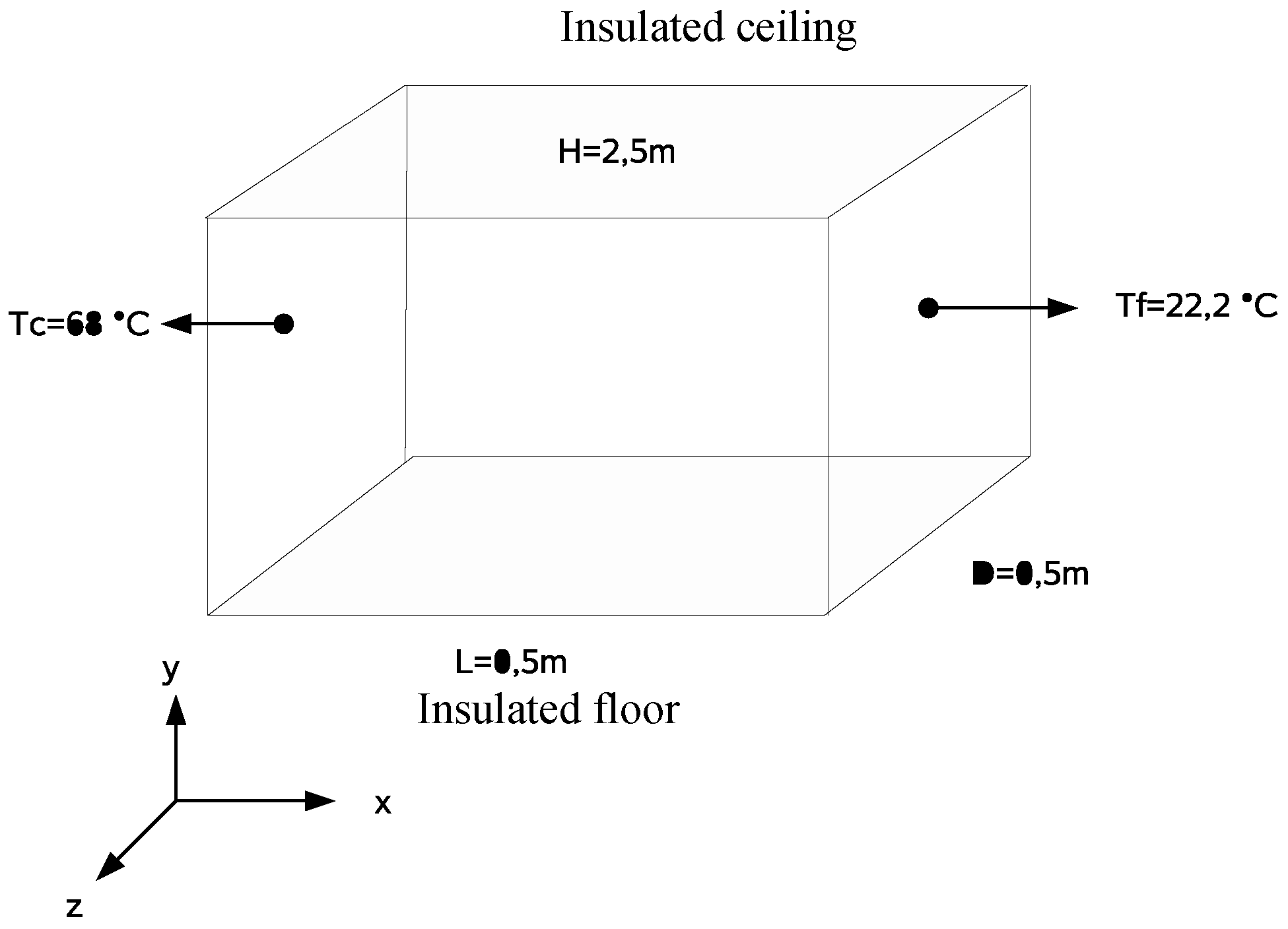
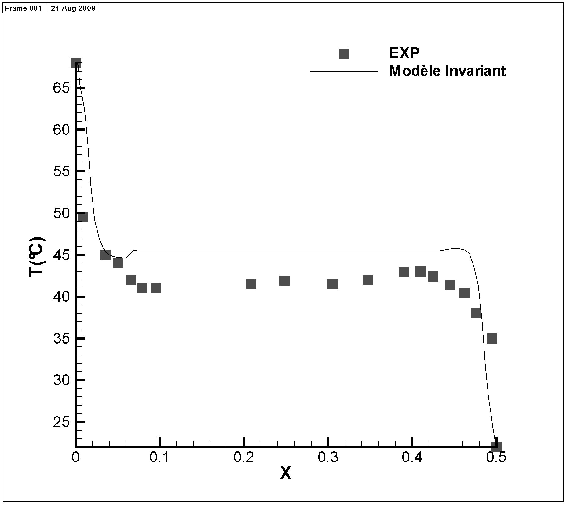
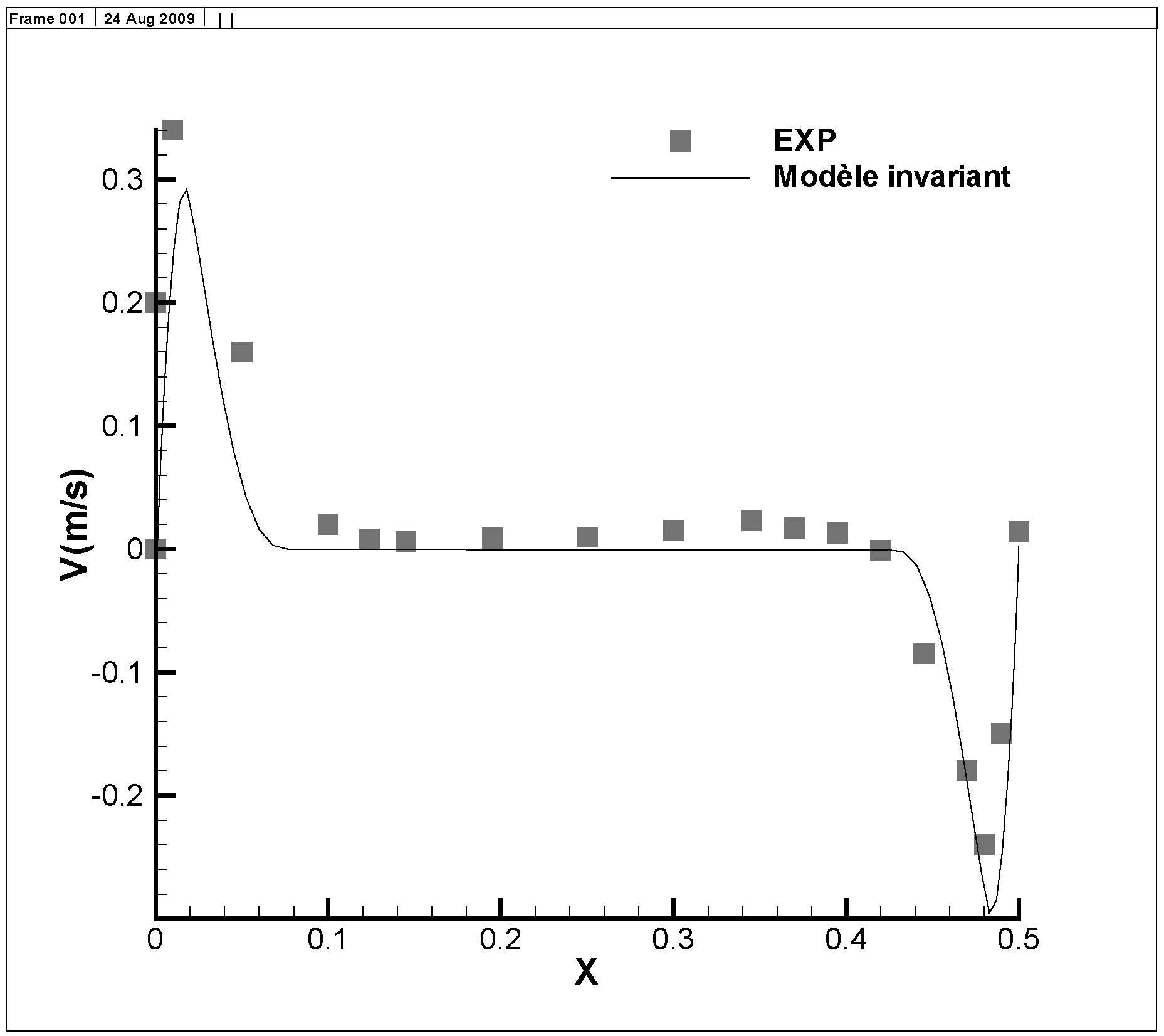
6. Numerical Example

Consider the case of an air flow in a differentially heated cavity (see Figure 1). The thermal expansion and the Prandtl number are such that

$$\beta g=0.03,\mathrm{and}{P}_r=0.711.$$

The code used for the simulation is based on a finite difference scheme, explicit in time [29]. The time step is 2$\times {10}^{-4}s$ and the grid size $(62\times 62\times 18)$. We use the experimental results in [30] as reference solution.

The mean temperature profile along an horizontal line, passing through the center of the cavity, is shown in Figure 2. It can be observed from it that the model can yield results that are quite close to the experimental data. This is more evident for the velocity profile which fits the experiment results, as seen in Figure 3. Note that these results were obtained with one of the simplest (linear) form of $g_m$ and $h_t$.

7. Conclusions

We proposed a way to build symmetry-consistent LES models, without using a Reynolds analogy for the subgrid heat flux. One of the most simple models was implemented numerically to serve as an example. In this example, it can be observed that the mean velocity profile obtained with the model is in good agreement with experiments, while the mean temperature is overestimated. A better choice of the functions $g_m$ and $g_t$ involved in (73) is to be analyzed in a future important work.

References

1. Nœther, E. Invariante Variationsprobleme. Königliche Gesellschaft der Wissenschaften 1918, 235–257. [Google Scholar]
2. Olver, P. Applications of Lie groups to differential equations (Graduate texts in mathematics); Springer-Verlag: New York, NY, USA, 1986. [Google Scholar]
3. Oberlack, M. A unified Approach for Symmetries in Plane Parallel Turbulent Shear Flows. J. Fluid Mech. 2001, 427, 299–328. [Google Scholar] [CrossRef]
4. Oberlack, M.; Cabot, W.; Pettersson Reif, B.; Weller, T. Group analysis, direct numerical simulation and modelling of a turbulent channel flow with streamwise rotation. J. Fluid Mech. 2006, 562, 355–381. [Google Scholar] [CrossRef]
5. Grassi, V.; Leo, R.; Soliani, G.; Tempesta, P. Vorticies and invariant surfaces generated by symmetries for the 3D Navier-Stokes equation. Physica A 2000, 286, 79–108. [Google Scholar] [CrossRef]
6. Ünal, G. Application of equivalence transformations to inertial subrange of turbulence. Lie Group Appl. 1994, 1, 232–240. [Google Scholar]
7. Speziale, C. Invariance of turbulent closure models. Phys. Fluids 1979, 22, 1033–1037. [Google Scholar] [CrossRef]
8. Speziale, C. Some interesting properties of two-dimensional turbulence. Phys. Fluids 1981, 24, 1425–1427. [Google Scholar] [CrossRef]
9. Fureby, C.; Tabor, G. Mathematical and physical constraints on large-eddy simulations. Theor. Comput. Fluid Dyn. 1997, 9, 85–102. [Google Scholar] [CrossRef]
10. Wang, L. Frame-indifferent and positive-denite Reynolds stress-strain relation. J. Fluid Mech. 1997, 352, 341–358. [Google Scholar] [CrossRef]
11. Spalart, P.; Speziale, C. A note on constraints in turbulence modelling. J. Fluid Mech. 1999, 391, 373–376. [Google Scholar] [CrossRef]
12. Pukhnachev, V. Invariant solution of Navier-Stokes equations describing motions with free boundary. Dokl. Akad. Nauk SSSR 1972, 202–302. [Google Scholar]
13. Oberlack, M. Symmetries of the Navier-Stokes equations and their applications for subgrid-models in large eddy simulation of turbulence. In Fundamental Problematic Issues in Turbulence; Gyr, A., Kinzelbach, W., Tsinober, A., Eds.; Birkhäuser Verlag: Basel, Switzerland, 1999. [Google Scholar]
14. Razafindralandy, D.; Hamdouni, A.; Oberlack, M. Analysis and development of subgrid turbulence models preserving the symmetry properties of the Navier–Stokes equations. Eur. J. Mech. B 2007, 26, 531–550. [Google Scholar] [CrossRef]
15. Razafindralandy, D.; Hamdouni, A.; Béghein, C. A class of subgrid-scale models preserving the symmetry group of Navier-Stokes equations. Commun. Nonlinear Sci. Numer. Simulat. 2007, 12, 243–253. [Google Scholar] [CrossRef]
16. Ibragimov, N. CRC handbook of Lie group analysis of differential equations. Vol 1: Symmetries, exact solutions and conservation laws; CRC Press: Boca Raton, FL, USA, 1994. [Google Scholar]
17. Cantwell, B. Similarity transformations for the two-dimensional, unsteady, stream-function equation. J. Fluid Mech. 1978, 85, 257–271. [Google Scholar] [CrossRef]
18. Lilly, D. A proposed modification of the Germano subgrid-scale closure method. Phys. Fluids 1992, A4, 633–635. [Google Scholar] [CrossRef]
19. Eidson, T. Numerical simulation of the turbulent Rayleigh-Bénard problem using subgrid modelling. J. Fluid Mech. 1985, 158, 245–268. [Google Scholar] [CrossRef]
20. Peng, S.H.; Davidson, L. Comparison of Subgrid-Scale Models in LES for Turbulent Convection Flow With Heat Transfer. In 2nd EF Conference in Turbulent Heat Transfer; Manchester, UK, 1998; Vol. 1, pp. 5.25–5.35. [Google Scholar]
21. Bardina, J.; Ferziger, J.; Reynolds, W. Improved turbulence models based on large eddy simulation of homogeneous, incompressible, turbulent flows. Technical Report Report TF-19; Stanford University: Standford, CA, USA, 1983. [Google Scholar]
22. Horiuti, K. The Role of the Bardina Model in Large Eddy Simulation of Turbulent Channel Flow. Phys. Fluids A 1989, 1, 426–428. [Google Scholar] [CrossRef]
23. Winckelmans, G.; Wray, A.; Vasilyev, O. Testing of a new mixed model for LES: the Leonard model supplemented by a dynamic Smagorinsky term. In Summer Program; Center for Turbulence Research, NASA Ames/Standford University: Standford, CA, USA, 1998; pp. 367–388. [Google Scholar]
24. Keating, A.; Piomelli, U.; Bremhorst, K.; Nesic, S. Large-Eddy Simulation of Heat Transfer Downstream of a Backward-Facing Step. J. Turbulence 2004, 5. [Google Scholar] [CrossRef]
25. Oberlack, M. Invariant modeling in large-eddy simulation of turbulence. In Annual Research Briefs; Stanford University: Standford, CA, USA, 1997. [Google Scholar]
26. Oberlack, M. Symmetries, Invariance and Scaling-Laws in Inhomogeneous Turbulent Shear Flows. Flow Turbul. Combust. 1999, 62, 111–135. [Google Scholar] [CrossRef]
27. Lindgren, B.; Österlund, J.; Johansson, A. Evaluation of Scaling Laws Derived from Lie Group Symmetry Methods in Zero-Pressure-Gradient Turbulent Boundary Layers. J. Fluid Mech. 2004, 502, 127–152. [Google Scholar] [CrossRef]
28. Razafindralandy, D.; Hamdouni, A. Invariant subgrid modelling in large-eddy simulation of heat convection turbulence. Theor. Comput. Fluid Dyn. 2007, 21, 231–244. [Google Scholar] [CrossRef]
29. Chen, Q.; Jiang, Y.; Béghein, C.; Su, M. Particulate Dispersion and Transportation in Buildings with Large Eddy Simulation. Technical report. Massachusetts Institute of Technology, 2001. [Google Scholar]
30. Zhang, W.; Chen, Q. Large eddy simulation of indoor airflow with a filtred dynamic subgrid scale model. Int. J. Heat Mass Transfer 2000, 43, 3219–3231. [Google Scholar] [CrossRef]
Figure 1. Differentially heated cavity.
Symmetry 02 00848 g001
Figure 2. Mean temperature profile at y = 1.25 m.
Symmetry 02 00848 g002
Figure 3. Mean velocity profile at y = 1.25 m.
Symmetry 02 00848 g003