Complex Networks and Symmetry I: A Review

Abstract

In this review we establish various connections between complex networks and symmetry. While special types of symmetries (e.g., automorphisms) are studied in detail within discrete mathematics for particular classes of deterministic graphs, the analysis of more general symmetries in real complex networks is far less developed. We argue that real networks, as any entity characterized by imperfections or errors, necessarily require a stochastic notion of invariance. We therefore propose a definition of stochastic symmetry based on graph ensembles and use it to review the main results of network theory from an unusual perspective. The results discussed here and in a companion paper show that stochastic symmetry highlights the most informative topological properties of real networks, even in noisy situations unaccessible to exact techniques.

1. Introduction

In this review and in a companion paper [1], we study several connections between symmetry and network theory. Most complex systems encountered in a diverse range of domains, from biology through sociology to technology, consist of networks of elements (vertices) connected together (by links, or edges) in an intricate way [2,3,4,5,6,7,8]. While graph theory started dealing with the mathematical description of network properties long ago [9], only recently massive datasets about large real-world complex networks have become available. This allowed an unprecedented activity of data analysis, which resulted in the establishment of some key ‘stylized facts’ about the structure of real networks, and motivated an intense theoretical activity aimed at explaining them.

Surprisingly (at least at the time when this was first observed), the empirically observed structure of real networks is strikingly different from what is obtained assuming simple homogeneous mechanisms of network formation, such as the traditional Erdős-Rényi random graph model [2,3]. In the latter, which will be an important reference throughout this review, every pair of vertices has the same probability p to be connected. This generates homogeneous topological features, such as a constant link density across the network, and a narrow (binomial) distribution of the degree k (number of edges reaching a vertex). By contrast, virtually any real network is found to display a modular structure, with vertices organized in communities tightly connected internally and loosely connected to each other, and a broad degree distribution, typically featuring a power-law tail of the form $P\left(k\right)\propto k^{-\gamma }$. Networks characterized by the latter property are called scale-free.

Besides the purely topological level, networks are also characterized by heterogeneous link weights. That is, the intensity of the connections is again broadly distributed, and non-trivially correlated to the topology. Capturing the richness of the information encoded in the weighted structure of networks is a hard task, and the definition of proper weighted structural properties an open problem [10,11,12]. At both the topological and the weighted level, many real networks are also characterized by an intrinsic directionality of their connections, which again implies that proper quantities must be introduced and measured in order to fully understand directed structural patterns [13,14,15].

As an additional level of complexity, dynamical processes generally take place on networks [4]. Remarkably, the heterogeneous structure of real networks has been found to determine major deviations from the behavior expected in the homogeneous case, which is the traditional assumption used to obtain predictions about the dynamics. As a consequence, most of these predictions have been shown to be incorrect when applied to real-world networks. A prototypic example of this discrepancy is found in models of epidemic disease spreading. When these models are defined on regular graphs, one finds that the transmission rate must overcome a finite epidemic threshold in order to guarantee the persistence of an infection. By contrast, on scale-free networks the value of the epidemic threshold vanishes, implying that a large class of diseases can escape extinction no matter their transmission rates, even if extremely low [4].

Finally, in some networks a feedback is present between the topology and the dynamics taking place on it. This is the case of adaptive networks, whose structure changes in response to their dynamical behavior, which is in turn affected by the structure itself [8]. Generally, adaptive networks cannot be properly understood by studying their topology and their dynamics separately, as simple models show [16].

It may appear that, due to the various levels of complexity encountered in the description of real networks, performing a symmetry analysis of these highly heterogeneous systems is likely to lead to a dead end. This is probably the reason why, although network theory developed very rapidly in recent years [2,3,4] and established tight connections with many other disciplines [5,6,7,8], its many relations to symmetry concepts have not been made explicit yet, apart from isolated examples [17,18,19,20]. On the other hand, one expects the formation of real networks to be guided by some organising principle, maybe non-obvious but surely not completely random, and possibly the result of evolutionary or optimisation mechanisms. This implies that network structure should encode some degree of order and symmetry, even if more general and challenging than the type found in geometrical objects. It is therefore important to introduce proper definitions of symmetries capturing the possible forms of organisation of real networks, and enabling a simplified understanding of the latter.

In this review we explore the connections between real networks and symmetry in more detail. We show that many of the approaches that have been proposed to characterize both real and model-generated networks can be rephrased more firmly in terms of symmetry concepts. To this end, in Section 2 we first clarify the peculiar notions of symmetry pertinent to real networks, which (unlike formal graphs studied in discrete mathematics) are always characterized by errors or imperfections. Then, in Section 3 we shall establish several connections between network theory and symmetry. Symmetry will be investigated over a wide range of invariances related to topological variables. The empirical result that in real networks some topological properties tend to distribute in structurally different ways from random networks, thus emphasizing a complex structure, will be rephrased in terms of symmetry concepts. Interestingly, Section 3 can be regarded as a brief review of network theory from the unusual perspective of the symmetry properties of real networks. Finally, in Section 4 we summarize our survey of network symmetries. In the companion paper [1], we exploit the concepts developed here to study stochastic symmetry in great detail in a particular case, and to address the problem of symmetry breaking in networks.

2. Types of Graph Symmetries

Before proceeding with a review of the empirical symmetries of real networks, we first distinguish between different notions of invariance we will be interested in. The mathematical definition of symmetry of an object is the set of transformations that leave the properties of the object unchanged. For instance, a straight line of infinite length is unchanged after displacing it along its own direction, and a circle is unchanged after rotating it around its center. Conversely, the transformations involved in the symmetries of an object can be exploited to define and construct the object itself: a straight line can be drawn by displacing a point along a chosen direction, and a circle can be drawn by rotating a point around a chosen center. In this case, one needs a unit (in both examples, a point) to iterate through the transformation. More complicated units lead to more complicated objects (for instance, rotating a whole disk rather than a single point leads to a torus).

2.1. Discreteness, Permutations, and More General Symmetries

In the case of graph symmetries, various considerations are in order. Firstly, a graph is a discrete object, and therefore the relevant transformations are discrete and not continuous as in the previous examples. An example of discrete transformation is the rotation of a square by an angle of $\pi /2$ radians (or a multiple) around its center: the square is symmetric under this discrete rotation but not under one with different angle, or under a continuous one. Similarly, a lattice (see Figure 1) is symmetric under a discrete displacement by a multiple of the lattice spacing (which maps all vertices to their nearest neighbours in a specified direction), but not under one with different length, or under a continuous one. We will discuss the discrete translational symmetry of networks in Section 3.1.

Secondly, graphs are topological objects, not geometrical entities: their properties are independent on the positions of vertices in some metric space, even if the graph itself may be the result of some position-dependent construction rule. Changing the positions (and sizes) of vertices, as well as changing the lengths (and widths) of links, only leads to a different visualisation of the same graph (see Figure 1), and has no effect on the topology of the latter (provided each link remains attached to the original vertices). Therefore the properties in terms of which one can check the symmetries of a graph are purely topological, and the set of transformations involved in such symmetries are purely relational. Whereas a geometric transformation (such as a translation or rotation) maps each point in a circle to a different point determined by its coordinates in the plane, a topological transformation maps each vertex in a graph to a vertex determined not by its coordinates but simply by its identity (i.e. its label): this transformation is merely a permutation of vertices. Permutations of vertices leading to the same topology are the automorphisms of a graph, and we will discuss them in Section 3.3. Nonetheless, if vertices are assigned coordinates in some embedding space, and the network construction depends on those coordinates (as for lattices), then the automorphisms are permutations induced by proper coordinate transformations (e.g. a translation). This is illustrated in Figure 1. Similar considerations apply if the graph construction depends on other properties, rather than positions, assigned to vertices (we will consider this case explicitly in Section 3.5). However, in many real-world cases one only knows the topology of the graph, and not the properties of vertices. In general, one does not even know whether vertices are actually assigned properties on which the structure of the network depends. In this case, all the automorphisms of the graph must be looked for by enumeration. The possibility that the complexity of real networks might be traced back to some simpler description involving hidden variables attached to vertices, whose transformations may induce symmetries that are not evident a priori, is an important aspect of network research, that we will discuss in Section 3.5. Therefore the general problem of graph automorphisms (Section 3.3) can take different forms depending on the nature of the (possible) properties inducing the symmetries of a particular network, as the two examples of translational symmetry (Section 3.1) and permutation of vertex properties (Section 3.5) show.

Thirdly, graphs may (or may not) exhibit symmetries under transformations that are not necessarily vertex permutations. An example is scale invariance (Section 3.2), which also applies to self-similar geometric objects, or fractals. In this case, the transformation is a change of scale in the description of the system. We will also encounter transformations that drastically change the topology of a graph, and only preserve some specified property such as the total number of links or the degrees of all vertices (Section 3.6). Finally, the transformations we will consider in Section 3.7 and Section 3.8 are vertex partitions and edge (rather than vertex) permutations respectively.

2.2. Stochastic Symmetry

As a final important remark we note that, when considering real networks rather than abstract graphs, one must take into account that the observed symmetry is in general only approximate. To illustrate this concept, let us consider the example of a real object of circular shape. While a perfect circle, as a mathematical entity, displays an exact rotational symmetry around its center, a real circle is unavoidably an approximate object, characterized by small imperfections. If we look for exact rotational symmetry in real circles, we have to conclude that no real object is circular, as perfect circles do not exist in reality. The paradox can only be solved by introducing an approximate notion of rotational symmetry, i.e. one where we allow rotated points to fall nearby existing points of the circle. Ultimately, this changes the picture substantially, since while a perfect circle can only be drawn by a perfectly rotating point (i.e. there is a unique trajectory defining the circle), an imperfect circle can be drawn following (infinitely) many trajectories. While there is a single perfect circle of given radius, there are infinite imperfect circles of given radius (and the definitions of circle and radius themselves also acquire an approximate meaning).

Thus, while we started investigating the symmetry of a single object, we naturally end up with a family of objects (containing the original one), all different from each other but nonetheless characterized by the same approximate symmetry. Remarkably, to define the symmetry of the single object, we need the entire family of its variants: while a rotation maps a perfect circle to itself, it maps an imperfect circle to a different imperfect circle. In particular, if we assume that a probability is associated with each approximate object (for instance, if we draw a circle by adding a small noise term in the radial direction), we end up with what is known as a statistical ensemble of objects. Objects ‘closer’ to the perfectly symmetric one are assigned larger probability, and objects deviating from the perfectly symmetric one by the same amount are equiprobable. A given real object is symmetric under the transformation considered if it is a typical (i.e. not unlikely) member of the ensemble defined by the transformation itself. This also means that, in order to detect deviations from symmetry in real objects, one needs an ensemble of imperfectly symmetric objects as a reference or null model. For instance, suppose one is investigating the properties of a real circle and a real square under rotational symmetry. If a perfect circle is assumed as the reference for a rotationally symmetric object, than both the real square and the real circle will be classified as non-symmetric. By contrast, if an ensemble of imperfect circles is considered as the null model, then the real square will still be classified as non-symmetric (since it is a very unlikely outcome of a circular null model) but the real circle will now be correctly classified as symmetric.

When applied to networks, the above considerations naturally lead to the notion of statistical ensembles of graphs, i.e. families of networks where each graph G is assigned a probability $P\left(G\right)$. We will encounter graph ensembles when considering either approximate equivalences or null models of real networks. As in the example above, a graph will be classified as exactly symmetric under a given transformation if it is mapped onto itself by the transformation (graph automorphism are an example of exact vertex permutation symmetry). By contrast, a graph will be classified as stochastically symmetric under a given transformation if it is a typical member of (i.e. well reproduced by) a graph ensemble which is stochastically symmetric under the same transformation. In the last definition, we consider a graph ensemble as stochastically symmetric under a transformation if the latter maps a graph $G_1$ in the ensemble into an equiprobable graph $G_2$ with $P\left(G_2\right)=P\left(G_1\right)$. Graph ensembles as null models of real networks will be introduced and discussed in Section 3.6, where we will also illustrate in more detail the idea of stochastic symmetry. We will also show that stochastic symmetry and entropy are intimately related in graph ensembles.

3. Symmetries in Real Networks

Thus there are various possible notions of symmetry one can look for in networks. In what follows, rather than discussing them in the order presented above, we follow a more pedagogical ordering, which allows us to trace the main results of network theory from the unusual perspective of symmetry. As we will try to elucidate, some symmetries are generally present in real networks, others are generally absent, and others are strongly network-dependent and variably observed. In some cases, even when a symmetry is present, it only holds within a limited range. All these situations are equally important, as they suggest what is relevant and what is not to plausible formation mechanisms involving a particular network. Our discussion provides a somewhat unconventional overview of this problem, and list a few examples (among possibly many more) of symmetries relevant to networks. Readers interested in a more comprehensive account of the results of network theory are referred to the relevant literature [2,3,4,8] and to the publications cited in the following text.

3.1. Translational Symmetry

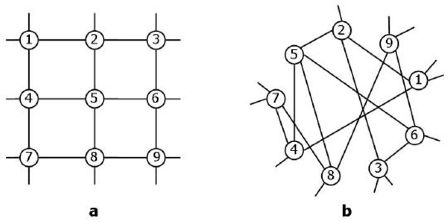
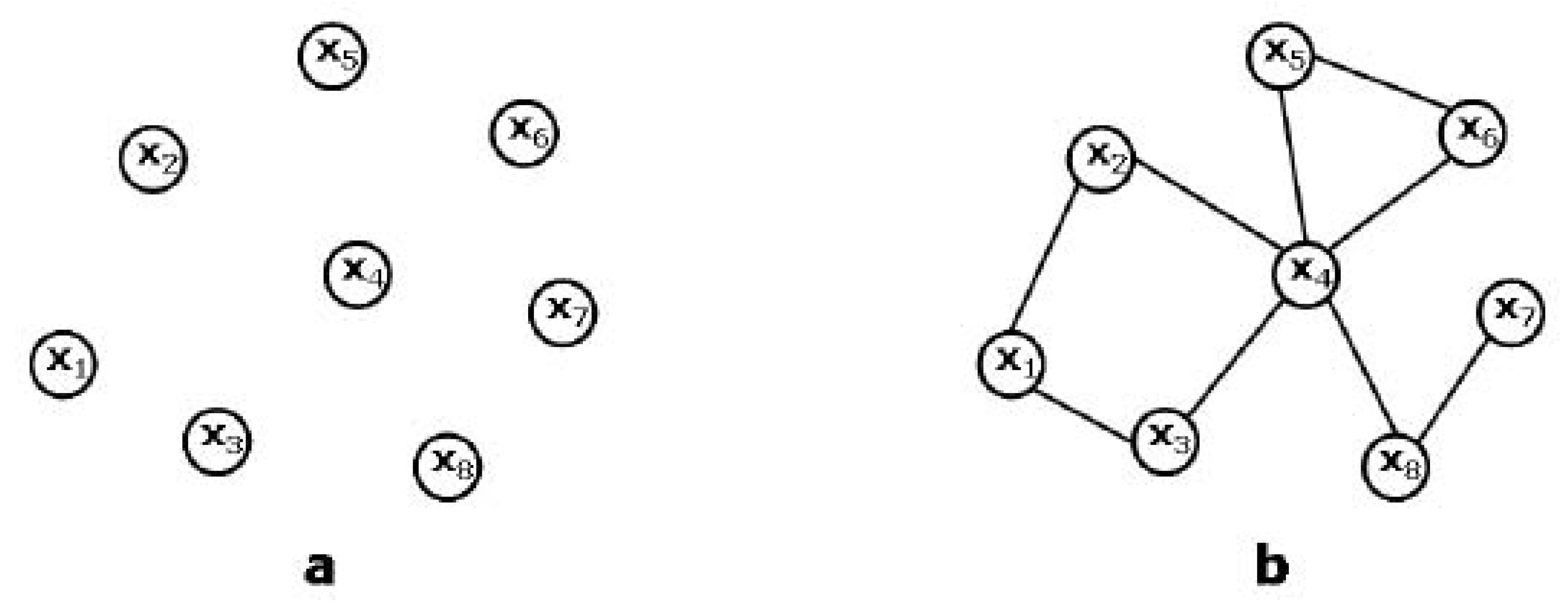
As we mentioned, some graphs may be embedded in a metric space where vertices are assigned positions. In this case, the symmetries (automorphisms) of a graph are induced by the transformations of coordinates in the embedding space, even if topologically their are simply permutations of vertices. This means that the topological properties of the graph, which are independent of the embedding space, will nonetheless reflect the properties of the latter. For instance, lattices are naturally formed by connecting vertices to their nearest neighbours in some embedding space (see Figure 1). A simple type of discrete symmetry encountered in (either infinite or periodic) regular lattices is translational symmetry. That is, the fact that the topology of a lattice embedded in some D-dimensional space does not change after a displacement by an integer multiple of the lattice spacing. Lattices are a particular type of regular graphs, i.e. graphs where every vertex has the same number of neighbours. 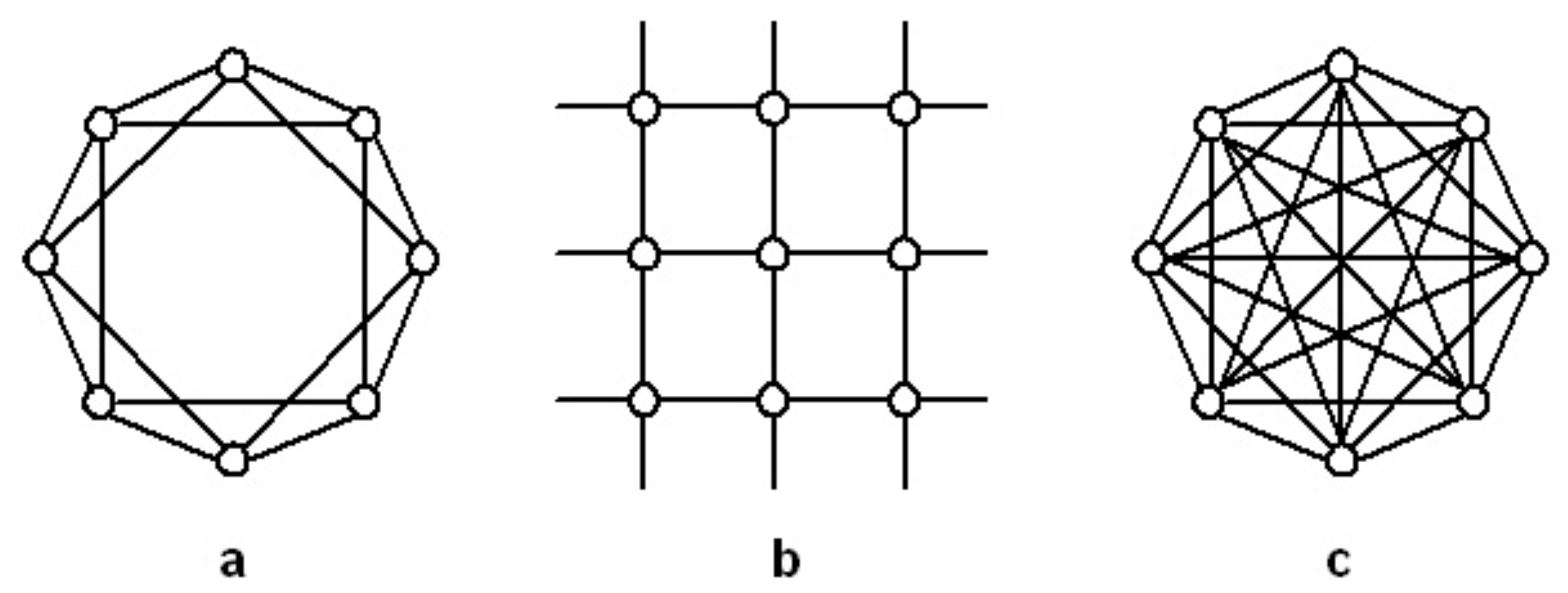In Figure 2 we show three examples of regular graphs embedded in different dimensions ($D=1$, $D=2$ and $D=\infty$) and with differently ranged connections (nearest neighbours, nearest and second-nearest neighbours, infinite neighbours).

If the labeling of vertices reflects their position in space, then translational symmetry is reflected in some regularities of the adjacency matrix A of the network (for undirected graphs, where no orientation is defined on the edges, the adjacency matrix A is a binary matrix whose entries equal $a_{ij}=1$ if a link between vertex i and vertex j is present, and $a_{ij}=0$ otherwise; here $i=1,\dots ,N$ where N is the total number of vertices, i.e. the size of the network). For instance, if the vertices are numbered cyclically along the ring, the adjacency matrices $A_a$ and $A_c$ of the graphs shown in Figure 2a and c read

$$A_a=\left(\begin{array}{cccccccc}0& 1& 1& 0& 0& 0& 1& 1\\ 1& 0& 1& 1& 0& 0& 0& 1\\ 1& 1& 0& 1& 1& 0& 0& 0\\ 0& 1& 1& 0& 1& 1& 0& 1\\ 0& 0& 1& 1& 0& 1& 1& 0\\ 0& 0& 0& 1& 1& 0& 1& 1\\ 1& 0& 0& 0& 1& 1& 0& 1\\ 1& 1& 0& 1& 0& 1& 1& 0\end{array}\right)A_c=\left(\begin{array}{cccccccc}0& 1& 1& 1& 1& 1& 1& 1\\ 1& 0& 1& 1& 1& 1& 1& 1\\ 1& 1& 0& 1& 1& 1& 1& 1\\ 1& 1& 1& 0& 1& 1& 1& 1\\ 1& 1& 1& 1& 0& 1& 1& 1\\ 1& 1& 1& 1& 1& 0& 1& 1\\ 1& 1& 1& 1& 1& 1& 0& 1\\ 1& 1& 1& 1& 1& 1& 1& 0\end{array}\right)$$

(1)

respectively. Translational symmetry is one of the traditional assumptions used in the theoretical study of discrete (or discretized) dynamical systems, and most of the available analytical results about dynamical processes are only valid under the assumption of the existence of this symmetry.

However, as one moves beyond the simple case of atoms regularly embedded in crystal lattices, virtually all real-world networks strongly violate translational symmetry. An important deviation from lattice-like topology in real networks is signaled by a surprisingly small value of the average inter-vertex distance, i.e. the average number of links one needs to traverse along the shortest path connecting two vertices. In most real networks, this quantity increases at most logarithmically with the number N of vertices, a phenomenon known as the small-world effect [2]. This behavior is also encountered in the random graph model mentioned in Section 1 but not in lattices, where the average distance (if infinite-ranged connections are not allowed, e.g. for the graphs in Figure 2a and b but not for that in Figure 2c) grows as $N^{1/D}$, thus much faster. The breakdown of translational symmetry implies that the wealth of knowledge accumulated in the literature about the outcome of dynamical processes on lattices cannot be applied to the same processes when they take place on real networks [4]. We already mentioned epidemic spreading processes as an example of the surprising deviation between dynamics on lattices and on more complicated networks. Nonetheless, real networks bear an interesting similarity with regular graphs, namely a large average value of the clustering coefficient, defined as the number of triangles (loops of length three) starting at a vertex, divided by its maximum possible value.

The simultaneous presence of a small average distance and of a large clustering coefficient (which is sometimes taken as a stronger definition of the small-world effect) has motivated the introduction of an important and popular network model which is somehow ‘intermediate’ between regular lattices and random graphs. In the model proposed by Watts and Strogatz [21], one starts with a regular lattice and then, with fixed probability p, goes through every edge and rewires one of its two end-point connections to a new, randomly chosen vertex. Clearly, when $p=0$ one has the original lattice (large clustering and large distance), while when $p=1$ one has a completely random graph (small clustering and small distance). Thus the parameter p can be viewed as a measure of the deviation from complete translational symmetry in the model. Interestingly, in a broad intermediate range of values one simultaneously obtains a large clustering and a small distance, thus recovering the empirically observed effect. This suggests that real networks may be partially, but surely not completely, affected by translational symmetry (due for instance to the existence of a natural spatial embedding). As we shall discuss in Section 3.5, translational symmetry, and in general the dependence of structural properties on the vertices’ positions in some embedding space, is an example of a more general situation where vertices are characterised by some non-topological quantity that may determine or condition their connectivity patterns.

3.2. Scale Invariance

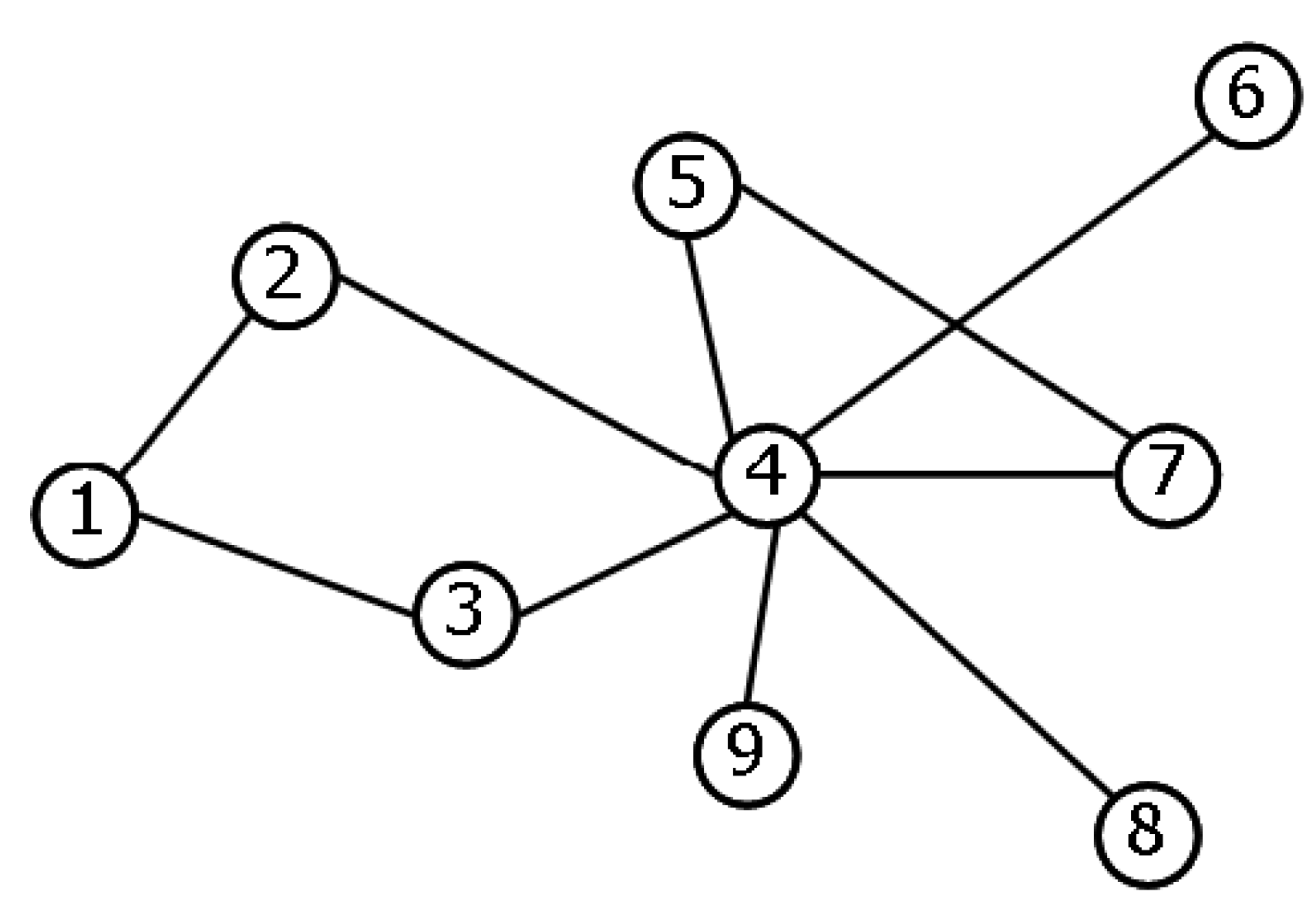
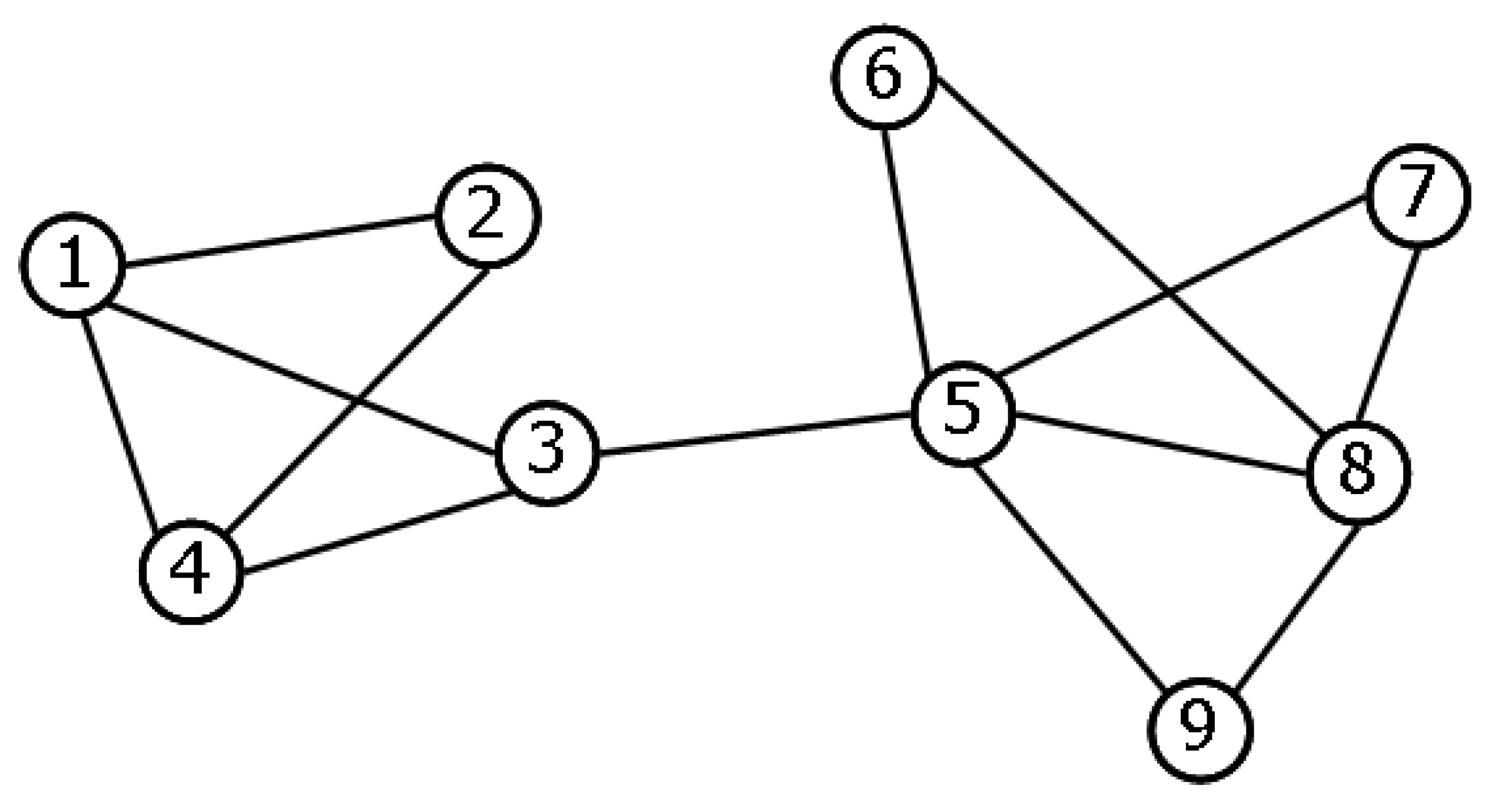
As we mentioned, one of the most striking and ubiquitous features of real networks is the power-law form $P\left(k\right)\propto k^{-\gamma }$ of the degree distribution. This property means that vertices are extremely heterogeneous in terms of their number of connections: many vertices have a few links, and a few vertices (the hubs) have incredibly many links. An example of a small network with highly heterogeneous degree distribution is shown in Figure 3. Importantly, most of the empirically observed values of the exponent $\gamma$ are found to be in the range $2<\gamma <3$, where the variance of the distribution diverges. This implies that there is no typical scale for the degree k in the system, and motivates the expression scale-free network [2].

The above property is an example of a remarkable type of symmetry, precisely scale invariance. It is found across different domains [22], and in particular in fractal objects. In fractals, scale invariance is manifest in the fact that iterated magnifications of an object all have the same shape, i.e. the system ‘looks the same’ at all scales. Similarly, in networks one finds that if the scale of the observation is changed (e.g. one switches from degree k to degree $ak$, with a positive), the number of vertices with given degree only changes by a (magnification) factor, from $P\left(k\right)$ to $P\left(ak\right)=a^{-\gamma }P\left(k\right)$. This is very different from exponential distributions, characterized by a strong variation in the number of counts as the scale is changed. In networks, power laws have also been found to describe the distribution of link weights, of the sum of link weights (the so-called strength) of vertices, and of many more quantities [2]. They also appear to hold across various coarse-grained levels of description of the same network, if groups of vertices are iteratively merged into ‘supervertices’ and the original connections collapsed into links among these supervertices [23]. The symmetry group associated to scale invariance, i.e. the renormalization group [24], has therefore been used many times to theoretically understand power-law distributed network properties.

The presence of a scale-free topology across several real-world networks, which is not reproduced by the Erdős-Rényi model and by the Watts-Strogatz one, has led to the introduction of new theoretical mechanisms that could possibly explain the onset of this widespread phenomenon. The earliest (even if analogous mechanisms were already known in different contexts [22]) and most popular scale-free network model is the one proposed by Barabasi and Albert [25]. It is based on two key ideas: firstly, networks can grow in time, therefore one can assume that new vertices are continuously added to a preexisting network; secondly, already popular (highly connected) vertices are likely to become more and more popular (‘rich get richer’). The latter idea, known as preferential attachment, is modeled as a multiplicative process in degree space: the probability that newly introduced vertices establish a connection to a preexisting vertex i is proportional to the degree $k_i$ of that vertex. The iteration of this elementary process of growth and preferential attachment eventually generates a power-law degree distribution of the form $P\left(k\right)\propto k^{-3}$. In degree space, preferential attachment is a symmetry-breaking mechanism: vertices are not equally likely to receive new connections as the network grows. Even if all vertices are identical a priori, preferential attachment determines and amplifies heterogeneities in the degree, and eventually vertices with different degrees become subject to different probabilistic rules. Since in the model there is a tight relationship between the degree of a vertex and the time the same vertex entered the network, one could also say that different injection times imply different expected topological properties. On the other hand, with respect to scale invariance, preferential attachment is symmetry-preserving and gives rise to a stationary process. Indeed, as the network grows infinitely in size over time, its scale-free degree distribution remains unchanged. This highlights how the same network properties may bear different meanings in relation to different symmetries. There are now many alternative models that reproduce scale-free networks with any value of the power-law exponent $\gamma$, not only $\gamma =3$ [2,3,8]. In all of them, there is some mechanism that eventually sets on and drives the network to converge to an extremely heterogeneous topology. We shall describe one of these models [26] in Section 3.5. Before doing that, in the following Section 3.3 and Section 3.4 we shall make a more general discussion about symmetry breaking due to differences in topological properties in a model-free and real-world framework.

3.3. Graph Automorphisms and Structural Equivalence

Various types of vertex permutation symmetry can be defined for graphs. Some of these symmetries are trivial, while others can be very interesting and informative. A trivial example is the symmetry under any overall permutation of vertex labels: if all vertices are relabelled differently, and a new adjacency matrix is defined accordingly, the resulting graph will have exactly the same topology of the original one (i.e. the two graphs are isomorphic to each other [9]). Since one is always free to assign any labelling to vertices, permutation symmetry trivially holds in any network (in mathematical words, an unlabelled graph is invariant under vertex relabelling). In this sense, a graph with N vertices is trivially invariant under the possible $N!$ permutations of vertex labels, if all edges are relabelled accordingly.

However, a far less trivial problem is whether, after a given labelling has been chosen (and the graph has therefore become a labelled one), the network still remains invariant under further vertex permutations. As we mentioned in Section 2, this is the graph automorphism problem, i.e. the analysis of the isomorphisms of a graph with itself [9]. Suppose the identity of every vertex has been fixed by assigning a unique label to each of them (as we mentioned, this labelling is arbitrary and every choice leads to an equivalent description of the same network). Once a labelling is chosen, one may still find that a particular graph is unchanged after permutations of some vertices (without exchanging the identity of the latter). Graph automorphisms are studied in detail by discrete mathematics. Technically, the set of vertex permutations defining the automorphisms of a graph forms a symmetry group, denoted as the automorphism group of the graph. Given a particular graph, the analysis of its automorphism groups provides a characterization of its properties, and in particular its symmetries. Traditionally, automorphism groups are studied for specific classes of graphs generated according to deterministic rules, which represent standard examples in graph theory [9]. The analysis of the automorphism groups of real-world networks is instead very recent [17,18,19,20]. One of the reasons why it is interesting to look for automorphisms in real networks is their relation to the following important problem. If two vertices i and j have exactly the same set of neighbors (irrespective of whether they are neighbors of each other), then a permutation exchanging i and j, and leaving all other vertices unchanged, leads to exactly the same graph. In social science, when this occurs the vertices i and j are said to be structurally equivalent [27]. In food web ecology (where also the direction of each link to the common neighbours must be the same), they are said to belong to the same trophic species [5,28]. An illustration of structural equivalence is shown in Figure 4. The adjacency matrix of a graph where i and j are structurally equivalent is unchanged after exchanging its ith and jth row, and its ith and jth column. In doing so, we are not interchanging the identity of i and j, which still represent the original vertices (for instance, two particular persons in a social network).

Structural equivalence, which may or may not be present in a given real network, is very important for many disciplines. It is directly related to the problem of network robustness: if a vertex is removed from the network, the presence of at least one structurally equivalent vertex warrants that there are no secondary effects (other vertices becoming disconnected) or major topological changes. By contrast, the effects can be dramatic if the removed vertex is a special one with no structurally equivalent peers (for instance, a highly connected hub). The analysis of the automorphism groups of real networks has revealed that, unlike random graphs, real networks are highly symmetric and contain a significant amount of structural redundancy [17,18,19,20]. This property may naturally arise from growth processes involved in the formation of many networks, and affects local topological properties such as network motifs (subgraphs of three or four vertices recurring in real networks much more often than in random graphs [29]). Graph automorphisms have also been used to simplify the topology of real networks by collapsing redundant information and obtaining network quotients [18], i.e. coarse grained graphs without structural repetition. Despite quotients of real networks are substantially smaller than the original graphs, they are found to preserve various structural properties (degree heterogeneity, small distance, etc.), effectively capturing a sort of skeleton of the entire empirical networks [18,20].

3.4. Statistical Equivalence

Structural equivalence is a very strict definition of similarity between two vertices. A more relaxed condition that is usually of interest in sufficiently large networks is whether two vertices are statistically equivalent, i.e. whether their topological properties are the same in an average or weak sense. For instance, one could ask whether two vertices i and j have simply the same degree (irrespective of the identity of their neighbors), and/or the same number of second neighbours, or whether they participate in the same number of triangles and/or longer loops. Similarly, one could be interested in finding two vertices whose neighbours have the same average degree, irrespective of the numbers of neighbours of each vertex, and of the individual values of the degrees of these neighbours (this is explained in more detail below). In all these examples, one focuses on a subset (or some average value) of the possible topological properties involving i and j, and defines an equivalence with respect to it only. According to this relaxed condition, a number of statistically equivalent vertices are found in real networks. The structure of the resulting equivalence classes determines the symmetry of a particular network. While permutations of structurally equivalent vertices are exact symmetries of the graph (i.e. automorphisms), permutations of statistically equivalent vertices are stochastic symmetries in the sense introduced in Section 2. Such transformations do not map a network to itself, but to another member of the family of networks with the same statistical properties. Importantly, while even small errors such as a missing link in the data have a dramatic effect on structural equivalence, statistical equivalence is more robust to fluctuations in network structure. Moreover, introducing this stochastic type of symmetry gives rise to identify more general patterns than those accessible to the analysis of structural equivalence. We discuss this concept by making some examples of the main scientific questions related to statistical equivalence in networks.

Do all vertices in a network have the same degree? As already discussed in Section 3.2, this type of symmetry is strongly violated in real networks. A weaker question would be: are the degrees of all vertices nearly the same? In this case, one could speak of a typical degree of vertices, and interpret the deviations from the average value as finite fluctuations due either to external noise or some intrinsic stochasticity. However, as we mentioned, the majority of real networks are scale-free, with degrees being broadly distributed and wildly fluctuating. There are many vertices with small degree, among which one can in principle find vertices with exactly the same number of neighbors, but also a few vertices with extremely large degree, which strongly break the symmetry.

Is the average degree of the neighbors of all vertices (nearly) the same? After recognizing that some vertices attract many more links than others, one can move one step forward and wonder what is the average degree of the neighbors of a given vertex (the so-called average nearest neighbor degree, or ANND [2]). This quantity encodes some information about the matching patterns in the network: if the degree plays no role in deciding whether two vertices are connected, then one expects that the ANND is independent of the degree itself (as we discuss below, this is not completely true). By contrast, one finds the presence of strong correlations between the degrees of neighboring vertices. These correlations can be either positive or negative, and have opposite effects on the ANND. In networks where large-degree vertices are more likely to be connected to each other than to low-degree ones, one observes an increasing trend of the ANND as a function of the degree. This property is known as assortativity [30]. In networks where the opposite is true, the ANND decreases with the degree, a situation denoted disassortativity. Importantly, degree-degree correlations have profound effects on the outcomes of dynamical processes taking place on networks [4].

Do all vertices have (nearly) the same clustering coefficient? Again, this symmetry is generally not observed, as vertices with different degree also have different values of the clustering coefficient. The latter usually displays a decreasing trend with the degree k. This behavior has been interpreted as the signature of a hierarchically organised topology, where a simple wiring pattern is repeated at different scales in a bottom-up fashion: first creating modules of vertices, then modules of modules, etc. [31]. Since both the clustering coefficient and the ANND strongly depend on the degree, and since the latter is broadly distributed, it appears that real networks are characterised by a high level of complexity, with no characteristic scale associated to any of the simplest topological properties one can define.

However, the last observation also leads to a reverse, possibly simplifying, approach to the problem. Interestingly, it has been shown that some of the correlations mentioned above are partly an unavoidable, ‘spurious’ outcome of enforcing some topological constraints in the network [32,33]. That is, exactly because many properties ultimately depend on the degree, a number of structural patterns are automatically generated once the degrees of all vertices are fixed to specified values. For instance, in networks with power-law degree distribution the ANND and the clustering coefficient both decrease with the degree. These patterns do not signal ‘true’ higher-order correlations, as they are natural outcomes due to the presence of simpler constraints. If an explanation from the latter exists, it also automatically explains the former. This highlights the importance of separating low-order effects from more fundamental higher-order structural patterns. This problem leads to the definition of suitable null models of networks, a point that we shall discuss in Section 3.6.

3.5. Invariance under Permutation of External Properties

An important type of permutation symmetry can be defined when some external, non-topological property is attached to vertices (or to edges, or to other subgraphs; but we will consider the case of vertices for simplicity). This situation is particularly relevant when one is interested in studying the relation between the topology and some other property characterising the vertices of a network, and is tightly related (even if in a nontrivial way) to structural and statistical equivalence, as the example in Figure 5 shows. Note that translational symmetry (described in Section 3.1) can be viewed as a particular case of this problem, if vertices are assigned positions in some metric space. Translational symmetry is in principle an exact symmetry (the graph is mapped onto itself) since it is the effect of a deterministic graph formation rule. However, symmetries due to external properties are in general stochastic in the sense discussed in Section 2, since real networks are always best understood as a result of non-deterministic rules. We therefore expect that stochastic symmetry is more powerful in detecting patterns in real networks than exact symmetry, and the following discussion confirms this expectation.

The impact of external factors is an extremely important problem, related to key questions about network formation, for many research areas. Typical examples include: is a social network partly determined by factors such as race, gender, age, etc.? Is wealth or income relevant to the formation of economic networks? In order to answer the above questions, one needs a way to assess the structural impact of properties which are in some sense external to the network.

There have been many attempts in this direction. Social network analysis has a long tradition in dealing with this problem, firmly based on statistical theory. The role of vertex properties is generally inspected through the values of regression parameters used in suitable graph models that are fitted to the real network [27]. More recently, in the physics community different approaches have been proposed. Techniques have been introduced [30,34] in order to capture whether the connections observed in a particular network occur mainly between vertices with similar properties (this is a generalised notion of assortativity, not necessarily related to vertices’ degrees, also known as homophily in social science) or between vertices with different properties (disassortativity). More generally, there have been attempts in understanding whether a specification of vertex properties effectively reduces the available configuration space for a real network [35] and can thus be interpreted as a structurally important factor. All these different approaches to the same problem could be restated in more general terms as follows: is the network (stochastically) symmetric under a permutation of the properties attached to vertices? If this is the case, the properties under consideration have no statistically significant impact on network structure. Otherwise, vertex-specific features are symmetry-breaking, as vertices with different properties are no longer equivalent under a somewhat generalised notion of the statistical equivalence described in Section 3.4. In particular, the overall permutation symmetry of vertex properties is broken and the network is only symmetric under a restricted set of permutations exchanging vertices within the same equivalence classes (sets of vertices with the same external properties). It is therefore clear that the behaviour of a network under the permutations associated to this type of permutation symmetry is determined by, and carries information about, the effects that external quantities have on the topology.

In general, the behaviour of a real network under permutation of external properties can be very complicated and lead to a variety of different symmetry properties. However, it is possible to understand the problem clearly in simplified models. Indeed, the idea that vertex properties may be crucial to network formation has led to the definition of an important class of network models known as fitness or hidden variable models [26]. Unlike the Barabasi-Albert model mentioned in Section 3.2, fitness models are static and do not require the hypothesis of network growth. 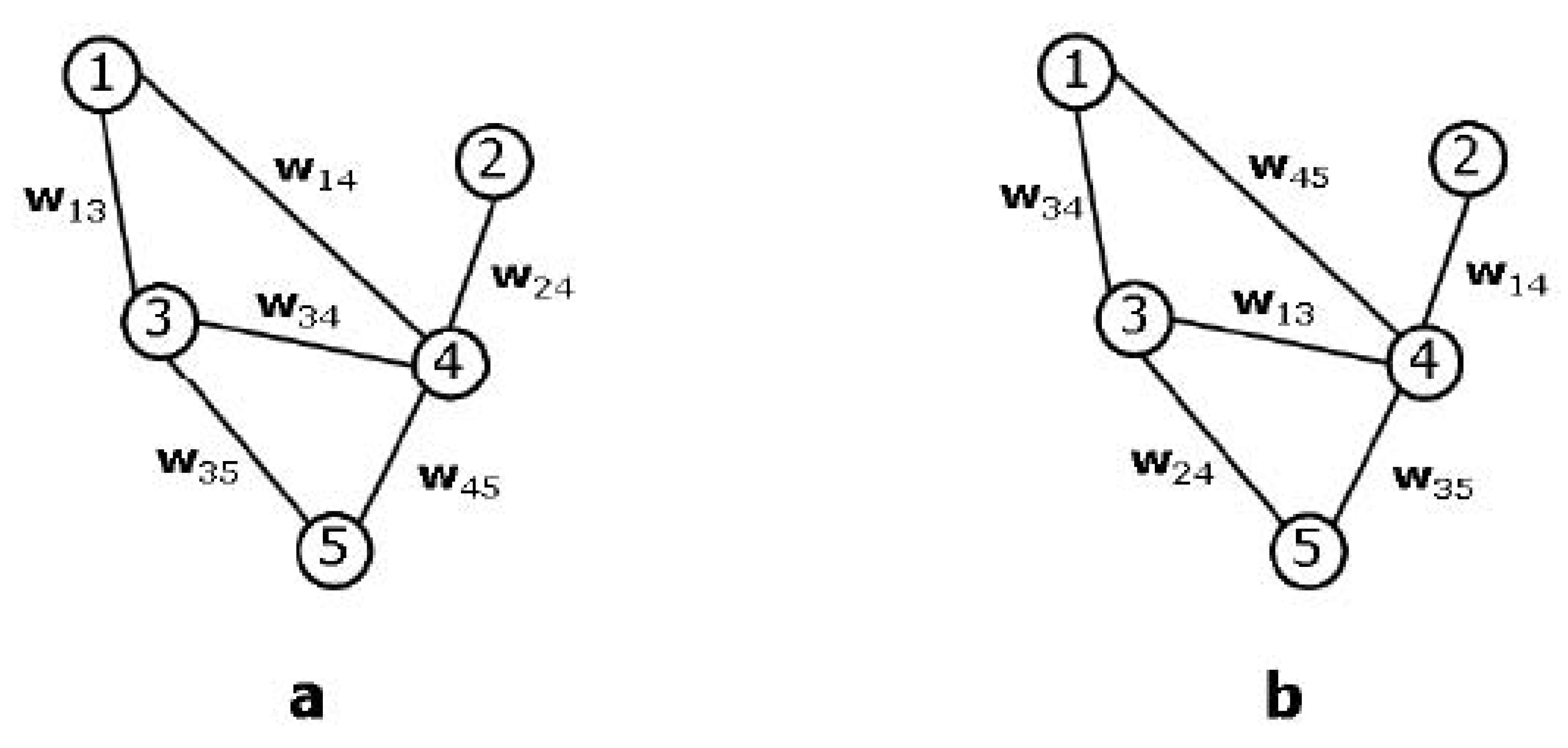In these models, one assumes that the probability $p_{ij}$ that a link is present between vertex i and vertex j is a function $p(x_i,x_j)$ of some property x, or fitness, attached to these vertices (see Figure 5). Therefore the model requires the specification of a list of fitness values $\left\{x_i\right\}$, usually assumed to be drawn independently from some probability distribution $\rho \left(x\right)$, and of the connection function $p(x_i,x_j)$. All the expected topological properties crucially depend on $\left\{x_i\right\}$. For instance, the expected degree of two vertices i and j with different fitness values ($x_i\ne x_j$) is in general different. On the other hand, two vertices with $x_i=x_j$ are statistically equivalent. However, due to the probabilistic nature of the model, in a particular realization of the network the statistical equivalence of vertices with equal fitness values does not necessarily reflects in their structural equivalence (see example in Figure 5). This model specification successfully reproduces the situation mentioned above, as the permutation symmetry of vertex properties is broken down to disjoint equivalence classes represented by sets of vertices with identical hidden values. Moreover, the flexibility in the choice of the fitness values and connection probability allows to reproduce various topological properties of real-world networks. For instance, a power-law distribution of fitness values (mimicking some heterogeneously distributed real-world feature such as individual wealth, country population, etc.) and a connection probability that linearly depends on the fitness naturally lead to a scale-free network topology [26]. Besides providing a valid route to network modelling, hidden variable models can also be fitted to real networks and shed light on the presence of external factors case by case [36,37]. In particular, inverse methods have been devised in order to extract, only from the topology of a real network, the values of the hidden variables $\left\{x_i\right\}$ potentially related to network formation. These values can then be compared with the values of candidate external properties relevant to that particular network, a strategy that has been shown to successfully identify key factors related to structure in real-world cases [36].

3.6. Ensemble Equiprobability

As we anticipated in Section 2, there are important symmetries associated not to a single graph, but to a statistical ensemble of graphs (we will define a graph ensemble rigorously below). If the ensemble is a good model of a real network, these symmetries can then be naturally related to the real network itself. This possibility allows us to illustrate in more detail our idea of stochastically symmetric ensemble, and the definition of stochastically symmetric graph as a network which is well reproduced by a stochastically symmetric ensemble (see Section 2). Null models automatically come into play when one is interested in understanding whether, in a given network, complicated high-order topological properties can be traced back to simpler low-level constraints. We already mentioned this problem in Section 3.4. In order to answer this question, it is necessary to consider a null model by generating a collection of graphs having some property in common with the real network (these properties act therefore as constraints), and being completely random otherwise. This amounts to generate an ensemble of graphs that maximizes an entropy, that we shall define in a moment, under the enforced constraints. Then, one can compare the properties of the real network with the corresponding averages over the randomised ensemble. If there is no statistically significant difference, one can conclude that the constraints considered are indeed enough in order to generate all the other properties of the real network. If differences are significant, then there are other factors shaping the observed topology. We now rephrase this idea more formally, and show how it highlights an intimate and instructive connection between symmetry, entropy and complexity in networks.

A statistical ensemble of graphs [38] is a collection of M graphs $\{G_1,G_2,\dots ,G_M\}$, each with an associated occurrence probability $P\left(G\right)$ satisfying

$$\sum _{G}P\left(G\right)\equiv \sum _{m=1}^{M}P\left(G_m\right)=1$$

(2)

We already mentioned examples of graph ensembles, without explicitly noticing it: Erdős-Rényi model (Section 1 and Section 3.1), the Watts-Strogatz model (Section 3.1), the Barabasi-Albert model (Section 3.2) and the fitness model (Section 3.5) are all examples of collections of possible graphs generated by probabilistic rules. The Barabasi-Albert model is a non-equilibrium ensemble, as it generates networks growing indefinitely in time; all the other examples mentioned above are instead equilibrium ensembles. In what follows, we restrict ourselves to the equilibrium case. Each graph G is uniquely specified by its adjacency (or weight) matrix, so we can think of G as of a matrix. For instance, if one is interested in the ensemble of binary undirected graphs with N vertices and no self-loops (edges starting and ending at the same vertex), then G will be a symmetric Boolean matrix with zeroes along the diagonal, and there will be $M=2^{N(N-1)/2}$ possible such matrices in the ensemble. In order to generate a maximally random ensemble of graphs with given constraints [38,39,40], one needs to find the form of the probability $P\left(G\right)$ that maximises the Shannon-Gibbs entropy

$$S\equiv -\sum _{G}P\left(G\right)\ln P\left(G\right)$$

(3)

(a standard measure of disorder or uncertainty) under the enforced constraints. The latter are a collection $\{c_1,\dots ,c_K\}$ of K topological properties, forming a K-dimensional vector $\overrightarrow{c}$. Each property $c_a$ ($a=1,\dots ,K$) evaluates to $c_a\left(G\right)$ when measured on the particular graph G. If the ensemble is meant as a null model of an empirical network $G^{*}$, the constraints will be chosen as the properties $\overrightarrow{c}\left(G^{*}\right)$ evaluated on the particular graph $G^{*}$.

There are various possible choices to solve the entropy maximisation problem, and different ensembles that one can define accordingly. If one is interested in matching the constraints exactly, i.e. in picking out only the graphs that have exactly the same properties as a given network $G^{*}$, then the solution is given by the probability

$$P\left(G\right)=\left\{\begin{array}{cc}1/\mathcal{N}\left[\overrightarrow{c}\left(G^{*}\right)\right]\hfill & \mathrm{if}\overrightarrow{c}\left(G\right)=\overrightarrow{c}\left(G^{*}\right)\hfill \\ 0\hfill & \mathrm{otherwise}\hfill \end{array}\right.$$

(4)

where $\mathcal{N}\left[\overrightarrow{c}\left(G^{*}\right)\right]$ is the number of graphs matching the constraints $\overrightarrow{c}\left(G^{*}\right)$. The above probability is uniform over the set of configurations matching the constraints exactly, and the resulting ensemble is known in statistical physics as the microcanonical ensemble. With the above choice, the entropy defined in Equation (3) takes the form

$$S=-\mathcal{N}\left[\overrightarrow{c}\left(G^{*}\right)\right]\frac{1}{\mathcal{N}\left[\overrightarrow{c}\left(G^{*}\right)\right]}\ln \frac{1}{\mathcal{N}\left[\overrightarrow{c}\left(G^{*}\right)\right]}=\ln \mathcal{N}\left[\overrightarrow{c}\left(G^{*}\right)\right]$$

(5)

which is known as the microcanonical entropy and is simply the logarithm of the number of configurations exactly matching the constraints.

A second alternative consists in requiring that the constraints $\overrightarrow{c}$ are matched on average, i.e. allowing any graph to occur with non-zero probability, provided that the expected value $\langle \overrightarrow{c}\rangle ={\sum }_{G}P\left(G\right)\overrightarrow{c}\left(G\right)$ of the constraints matches the required value $\overrightarrow{c}\left(G^{*}\right)$. This problem can be solved introducing Lagrange multipliers $\{{\theta }_1,\dots ,{\theta }_K\}$, each associated to one of the constraints. The solution is the probability distribution

$$P\left(G\right)=\frac{e^{-H\left(G\right)}}{Z}$$

(6)

where $H\left(G\right)$ (the graph Hamiltonian) is a linear combination of the constraints

$$H\left(G\right)\equiv \sum _{a=1}^K{\theta }_a{c}_a\left(G\right)$$

(7)

and Z is the partition function that properly normalizes the probability:

$$Z\equiv \sum _G{e}^{-H\left(G\right)}$$

(8)

Thus both Z and $P\left(G\right)$ depend on the K parameters $\{{\theta }_1,\dots ,{\theta }_K\}$. The ensemble generated by the above probability is known in physics as the canonical ensemble. For a given choice of the parameters $\{{\theta }_1,\dots ,{\theta }_K\}$, the expected value of a topological property X across the ensemble is

$$\langle X({\theta }_1,\dots ,{\theta }_K)\rangle \equiv \sum _{G}P\left(G\right)X\left(G\right)$$

(9)

(throughout this review, the angular brackets $\langle ·\rangle$ will denote ensemble averages). In order to match the constraints $\overrightarrow{c}\left(G^{*}\right)$ on average, the K parameters $\{{\theta }_1,\dots ,{\theta }_K\}$ must be set to the particular values $\{{\theta }_1^{*},\dots ,{\theta }_K^{*}\}$ such that

$$\langle c_a({\theta }_1^{*},\dots ,{\theta }_K^{*})\rangle =c_a\left(G^{*}\right)a=1,\dots ,K$$

(10)

Importantly, the above parameter choice corresponds with what the maximum likelihood principle would indicate [36], i.e. with the values maximising the probability $P\left(G^{*}\right)$ to obtain the real network $G^{*}$ under the model considered. We will indicate the maximum-likelihood parameter choice explicitly in the examples considered later on. It has been shown [38] that the canonical ensemble of networks coincides with the exponential random graph models that have been first introduced in social science [27]. The Hamiltonian $H\left(G\right)$ represents the energy, or cost, associated with a given configuration, and contains all the information required in order to formally obtain $P\left(G\right)$. This means that any two graphs $G_1$ and $G_2$ for which

$$H\left(G_1\right)=H\left(G_2\right)$$

(11)

have the same ensemble probability $P\left(G_1\right)=P\left(G_2\right)$. Thus, the symmetries of $H\left(G\right)$ are transformations connecting equiprobable graphs in the ensemble. Such transformations map a graph $G_1$ into a graph $G_2$ which has a different topology but exactly the same values of the enforced constraints. According to our definition in Section 2, a canonical graph ensemble is stochastically symmetric under such transformations. If a canonical graph ensemble is a good model of a real network $G^{*}$, the latter is also stochastically symmetric. Maximally random graphs with constraints therefore represent ideal candidates to illustrate the concept of stochastic symmetry. The symmetries of the Hamiltonian, together with the parameter values enforcing the constraints, determine the entropy S of the ensemble. This entropy is a measure of the residual uncertainty about the detailed topology of a network, once the constraints are fixed.

In statistical physics, there is also a third class of ensembles, i.e. grandcanonical ensembles. In the latter, the number of particles of the system is also allowed to vary, and it is treated as one of the properties to be matched on average. In the case of networks, the role of particles is played by links [38], whose number is allowed to vary already in the canonical ensemble, as the examples considered below illustrate. Therefore there is no fundamental difference between the canonical and grandcanonical ensembles of graphs, unless one is interested in networks with different types of links [14]. For large systems, the microcanonical, canonical and grandcanonical ensembles give very similar results. The canonical and grandcanonical ensembles have the enormous advantage to be analytically treatable, as a consequence of the relaxed requirement on the constraints. For this reason, in what follows we shall consider (grand)canonical ensembles of graphs.

We now discuss some examples. If we consider again the ensemble of all possible undirected graphs with N vertices, the completely symmetric case is the one where each graph G has the same energy

$$H\left(G\right)=H_0$$

(12)

where $H_0$ is a constant. In other words, in this case there are no constraints. Clearly, each of the M possible graphs has the same probability

$$P\left(G\right)=2^{-N(N-1)/2}$$

(13)

and therefore the graph probability is uniformly distributed across the ensemble (in this particular case, the microcanonical and canonical ensembles coincide). Transformations changing a graph G into any other graph in the ensemble are symmetries of the Hamiltonian, and lead to the same ensemble probability. Thus this ensemble is stochastically symmetric under any transformation. The entropy is the maximum possible, and its value is

$$S=\frac{N(N-1)}{2}\ln 2$$

(14)

A different case is when there is a constraint on the total number of links $L={\sum }_{i<j}{a}_{ij}$. Then

$$H\left(G\right)=\theta L\left(G\right)$$

(15)

and it can be easily shown that

$$P\left(G\right)=p^{L\left(G\right)}{(1-p)}^{N(N-1)/2-L\left(G\right)}$$

(16)

where $p\equiv e^{-\theta }/(1+e^{-\theta })$. This shows that, as expected, two graphs $G_1$ and $G_2$ with the same number of links $L\left(G_1\right)=L\left(G_2\right)$ are equiprobable. Graph transformations preserving this number are symmetries of the Hamiltonian, and the ensemble is stochastically symmetric under such transformations. Equation (16) indicates that, for each of the $N(N-1)/2$ pairs of vertices, the probability of an undirected link being there is p. The probability of exactly $L\left(G\right)$ realised edges is $p^{L\left(G\right)}$ multiplied by the probability ${(1-p)}^{N(N-1)/2-L\left(G\right)}$ of the complementary number $N(N-1)/2-L\left(G\right)$ of missing edges. This case is therefore equivalent the Erdős-Rényi random graph model that we already mentioned in Section 1, in which each edge is drawn, independently of each other, with probability p. The entropy of the ensemble now depends on p, and one can easily see that if $p=1/2$, Equation (14) is recovered. Indeed, this is the case where each edge is equally likely to be present and absent, which is another way to say that no constraint has been enforced and the entropy is maximum. By contrast, in the two cases $p=0$ and $p=1$ the entropy is $S=0$ as there is no uncertainty about the resulting structure of the network. Indeed, in these cases the ensemble completely shrinks to the only possible network, i.e., the empty graph and the complete graph respectively. If one wants to use the random graph model as a null model of a real network $G^{*}$, the maximum likelihood principle applied to Equation (16) indicates [36] that the parameter p must be set to the value

$$p^{*}=\frac{2L\left(G^{*}\right)}{N(N-1)}$$

(17)

which ensures that the expected number of links $\langle L\rangle$, as defined by Equation (9), reproduces the number of links $L\left(G^{*}\right)$ of that particular network:

$$\langle L\rangle =p^{*}\frac{N(N-1)}{2}=L\left(G^{*}\right)$$

(18)

In the random graph model, the expected degree distribution is binomial (in the large network limit with fixed average degree, Poissonian) with mean $p^{*}(N-1)=2L\left(G^{*}\right)/N$. The failure of the random graph model in reproducing the properties of real networks, according to our discussion in Section 1, can then be restated as the inefficacy of specifying the number of links as the only property of a network. This also means that real networks are generally not stochastically symmetric under transformations preserving the total number of links. A less trivial choice is the so-called configuration model [32,41]. Assuming we are still interested in undirected binary networks, the configuration model is a maximally random graph ensemble where the degrees of all vertices, i.e. the degree sequence $\left\{k_i\right\}$, are specified. Note that, in terms of the adjacency matrix A of the graph, the degree of vertex i is $k_i={\sum }_j{a}_{ij}$, and the total number of links is twice the sum of the degrees of all vertices: $L={\sum }_{i<j}{a}_{ij}={\sum }_i{k}_i/2$. Therefore specifying the degree sequence automatically fixes also the total number of links, which confirms that this model is more constraining than the random graph one. The configuration model naturally comes into play in the problem we described in Section 3.4, when we stressed the importance of comparing a real network to a null model in order to separate genuine higher-order correlations from mere effects of low-level constraints. The degree sequence is an important constraint to consider, because the widespread occurrence of scale-free architectures implies that major topological differences across real networks must be looked for in other properties beyond the degree distribution. Note that specifying the degree sequence $\left\{k_i\right\}$ is different from specifying the degree distribution $P\left(k\right)$. A given degree sequence generates a unique degree distribution, but there are many degree sequences ($N!$ permutations) generating the same degree distribution. Therefore fixing the degree distribution is less informative than specifying the entire degree sequence, and we do not consider it here. For directed graphs, the configuration model is naturally extended by simultaneously considering as constraints the number of incoming links (in-degree) and the number of outgoing links (out-degree) of all vertices. Similarly, for weighted networks the constraints become the strength (total edge weight) of all vertices (the strength sequence), or the corresponding directed quantities when applicable.

In the binary undirected case, the Hamiltonian of the configuration model contains the degrees of all vertices:

$$H\left(G\right)=\sum _{i=1}^N{\theta }_i{k}_i\left(G\right)$$

(19)

and it can be shown [33] that the form of $P\left(G\right)$ determined by the above choice is

$$P\left(G\right)=\prod _{i<j}{p}_{ij}^{a_{ij}\left(G\right)}{(1-p_{ij})}^{1-a_{ij}\left(G\right)}=\frac{{\prod }_i{x}_i^{k_i\left(G\right)}}{{\prod }_{i<j}(1+x_i{x}_j)}$$

(20)

where

$$p_{ij}=\frac{x_i{x}_j}{1+x_i{x}_j}$$

(21)

and $x_i\equiv e^{-{\theta }_i}$ is another way to write the Lagrange multiplier associated to $k_i$. In this model, edges are still independent, but have different probabilities.

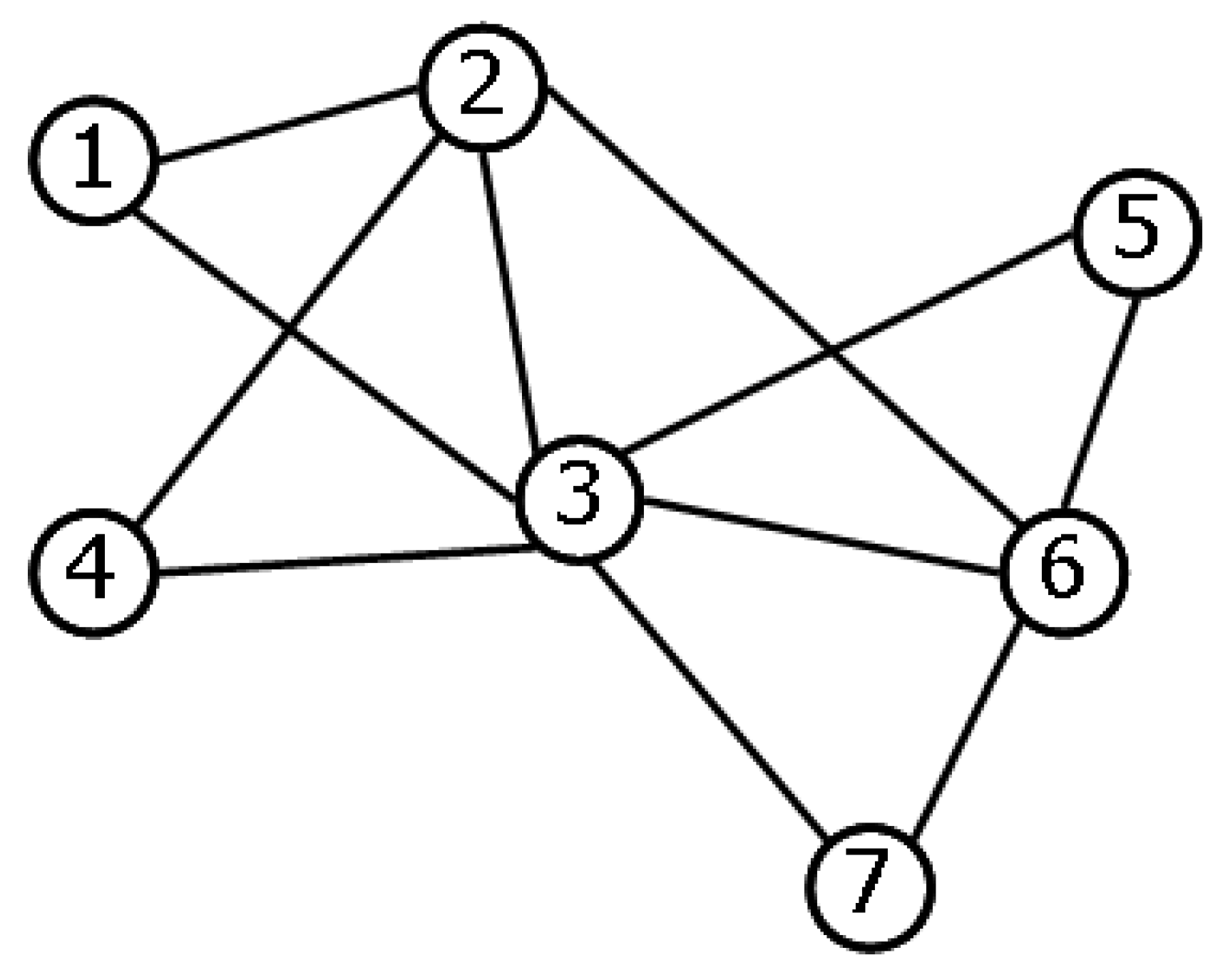
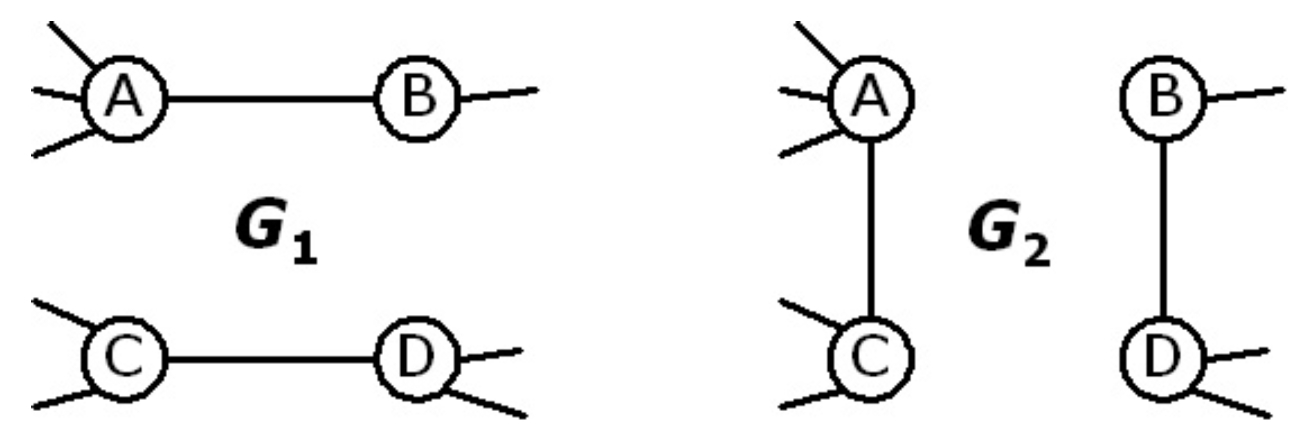
The probability $P\left(G\right)$ of a graph G only depends on its degree sequence, as evident from Equation (20). Thus any two graphs $G_1$ and $G_2$ with the same degree sequence $\left\{k_i\left(G_1\right)\right\}=\left\{k_i\left(G_2\right)\right\}$ are equiprobable in the ensemble specified by Equation (19). A consequence of this property is illustrated in Figure 6, where we show two graphs $G_1$ and $G_2$ that have exactly the same topology, except for the two edges shown. Graph $G_2$ can be obtained from $G_1$ by replacing the two edges $(A-B)$ and $(C-D)$ with the two edges $(A-C)$ and $(B-D)$. Since this transformation preserves the degree sequence, it is a symmetry of the Hamiltonian defined in Equation (19) and connects equiprobable graphs. According to our definition in Section 2, the ensemble is stochastically symmetric under such transformation. The equivalence classes of this symmetry are sets of graphs with the same degree sequence.

This property has been used to constructively define an algorithm that randomises a real network $G^{*}$ by iteratively selecting a pair of edges and swapping the end-point vertices exactly as in Figure 6 [32]. This procedure, known as the local rewiring algorithm, ergodically explores the equivalence class where the real network $G^{*}$ belongs. Any topological property of interest can be averaged across the set of graphs produced by the algorithm and compared with the value of the same property in the original graph $G^{*}$. This allows to check the effects of the degree sequence alone on the other topological properties. As we mentioned, this null model is restricted to only one equivalence class of the symmetry (it is a microcanonical ensemble), and requires that averages are numerically performed over the graphs sampled by the local rewiring algorithm. By contrast, the null model defined by Equation (19) explores the entire set of $2^{N(N-1)/2}$ undirected graphs (it is a (grand)canonical ensemble), and allows to obtain the expectation values analytically through Equation (9). This requires that the parameters $\{x_1,\dots ,x_N\}$ are set to the values $\{x_1^{*},\dots ,x_N^{*}\}$ that maximise the likelihood to obtain the real network $G^{*}$ [36,42]. These values are found by solving the following N coupled equations

$$\langle k_i\rangle =\sum _{j\ne i}\frac{x_i^{*}{x}_j^{*}}{1+x_i^{*}{x}_j^{*}}=k_i\left(G^{*}\right)\forall i$$

(22)

ensuring that the expected degree sequence coincides with the observed one, and thus generalising Equation (18). As we already anticipated in Section 3.4, an important conclusion drawn from the analysis of the configuration model is that, if real-world scale-free degree distributions are specified, higher-order patterns are automatically generated. In particular, the average nearest neighbour degree and the clustering coefficient of a vertex with degree k are both found to decrease with k [32,33,42]. These patterns should not be interpreted necessarily as the result of additional mechanisms, beyond those required to explain the form of the degree distribution. Note that if a real network is found to be well reproduced by the configuration model, then it is stochastically symmetric under transformations preserving the degree sequence. Also note that any two vertices i and j with the same degree $k_i\left(G^{*}\right)=k_j\left(G^{*}\right)$ in the real network are statistically equivalent in the sense specified in Section 3.4. This is because Equation (22) implies that those vertices would be assigned the same parameter value $x_i^{*}=x_j^{*}$, and would therefore have the same expected topological properties as discussed for the fitness model in Section 3.5. Whereas permutations of structurally equivalent vertices lead to exactly the same topology and are therefore automorphisms (exact symmetries) of the network, permutations of statistically equivalent vertices (here, vertices with the same degree) are stochastic symmetries of the network, if the latter is in accordance with the configuration model. This is an interesting and important relation between ensemble equiprobability, symmetry under permutation of vertex properties, and statistical equivalence. If the ensemble is not a good model of the real network, which signals the presence of mechanisms that break the postulated equiprobability symmetry, then the real network is not stochastically symmetric under transformations preserving the degree sequence, and vertices displaying the same values of the enforced constraints are no longer statistical equivalent.

Note that Equation (20) generalises Equation (16), and also that Equation (21) can be viewed as a particular case of the connection probability $p(x_i,x_j)$ introduced in the fitness model we described in Section 3.5. Indeed, the configuration model and the fitness model both reduce to the random graph case if $x_i=x_0$ $\forall i$, i.e. if all vertices have the same properties. In this case, the entropy associated with Equation (21) coincides with the one associated with Equation (16). By contrast, if the $x_i$’s are heterogeneously distributed, the entropy is significantly decreased. In particular, the values of the $x_i$’s required in order to enforce a scale-free degree distribution as observed in real networks are approximately power-law distributed, a result implying a strong reduction of the entropy of the ensemble associated with the degree sequence of real networks. In particular, it was shown that networks with degree distribution $P\left(k\right)\propto k^{-2}$ have remarkably small entropy [39] and can be generated deterministically [26] like regular graphs. We therefore see that network complexity, as signalled in this example by a scale-free degree distribution, can lead to a decrease in the stochastic symmetry associated with ensemble equiprobability, and to a substantial decrease in the corresponding entropy. From the perspective of the amount of information required in order to reproduce them, real networks (and possibly many real complex systems) turn out to achieve an unsuspected degree of order by following a nontrivial path, which is completely different from that taken by regular structures.

3.7. Symmetry under Network Partitioning: Modularity and Communities

As we briefly mentioned in Section 1, real networks are found to display inhomogeneous link density, and to be partitioned into communities of vertices [43]. Several different definitions of a community have been introduced. Generally, these definitions try to capture different aspects of the same simple idea: that communities are more densely connected internally than with other communities, so that intra-community links are typically denser than inter-community ones. An example is shown in Figure 7 to illustrate this concept. This simple idea can however give rise to technical difficulties when implemented into community detection algorithms and applied to large networks, and as a result different methods have been developed, each dealing with a different aspect of the problem. For instance, some methods try to identify the optimal partition of vertices into non-overlapping subsets representing communities; others recognise that the optimality of a partition depends on the resolution adopted, and give a multi-resolution output where communities are hierarchically nested into each other; others are devised to identify overlapping communities, etc. Presenting the subtleties and diversity of the community detection problem is beyond the scope of the present review, and the interested reader is referred to the relevant literature [43]. We simply note here that the community structure of a network is connected to a particular type of symmetry: the invariance under network partitioning. To illustrate this idea, we consider as an example a widely used quantity that measures the goodness of a partition of a real undirected network into non-overlapping communities, i.e. the modularity

$$Q\equiv \frac{1}{L}\sum _{i<j}(a_{ij}-p_{ij})c_{ij}$$

(23)

In the above definition, $a_{ij}$ is the entry of the adjacency matrix A of the real network, $L={\sum }_{i<j}{a}_{ij}$ is the observed number of links, $p_{ij}$ is the probability that vertices i and j are connected under a null model chosen as a reference, and $c_{ij}$ indicates if in the partition under consideration vertices i and j are placed in the same community ($c_{ij}=1$) or in different communities ($c_{ij}=0$). Typically, the null model considered is the configuration model (see Section 3.6). Since different partitions of the same network correspond to different sets of values $\left\{c_{ij}\right\}$, Q can be used to assess the performance of a partition in correctly placing in the same community ($c_{ij}=1$) pairs of vertices that are connected ($a_{ij}=1$) despite the null model predicts a low connection probability ($p_{ij}\approx 0$), and in placing in different communities ($c_{ij}=0$) pairs of vertices that are not connected ($a_{ij}=0$) despite the null model predicts a high connection probability ($p_{ij}\approx 1$). Larger values of Q represent better partitions. If the network is well reproduced by the null model, then one expects a value of Q close to zero, independently of the partition. To see this, imagine that the network has indeed been generated by the null model. If several realisations of the network are generated, then the expected value pf $a_{ij}$ is $p_{ij}$ and the expected modularity is

$$\langle Q\rangle =0$$

(24)

independently of $c_{ij}$. This means that a network with no community structure is stochastically invariant (in the sense specified in Section 2) under vertex partitioning, as all reassignments of vertices to different communities preserve on average the modularity. The modular structure of real networks can be therefore seen as a symmetry-breaking property. In some networks, the maximisation of the modularity can be very complicated numerically, as there are many competing partitions with similar values of Q (computationally, finding the partition corresponding to the global maximum of Q is a NP-hard problem). This indicates that in real networks the overall invariance under partitioning is often broken down to equivalence classes containing partitions with approximately equal modularity.

3.8. Edge Weight Permutation Invariance

As the last example of symmetries in networks, we consider an invariance that naturally comes into play in the analysis of weighted networks. Weighted networks are described by a non-negative matrix W rather than by a binary adjacency matrix A. The entry $w_{ij}$ of the matrix W represents the weight of the edge from vertex i to vertex j (if $w_{ij}=0$ no edge is there). In the analysis of weighted networks, a crucial point is assessing whether the knowledge of edge weights indeed conveys additional information with respect to the knowledge of the binary topology. This problem has been tackled by introducing suitable definitions of structural properties that make explicit use of the empirical edge weights and that distinguish between the real network and suitably randomised counterparts [10,11,12].

The randomised case can be either a weighted generalisation of the maximally random networks described in Section 3.6 [40], or a different null model providing a reference where weights and topology are uncorrelated, so that weighted properties reduce to simpler binary properties [10]. The latter null model consists in taking the real network, keeping its topology fixed, and randomly reshuffling the values of the weights across the edges (see Figure 8).

Iterating this procedure generates an ensemble of randomised networks where any correlation existing between weights and topology is destroyed. This provides a reference for the analysis of the original real network. A prototypical example of the deviation of real networks from the uncorrelated case is the generally observed power-law relation between the degree $k_i={\sum }_{j\ne i}{a}_{ij}$ and the strength $s_i={\sum }_{j\ne i}{w}_{ij}$ of vertices:

$$s_i\propto k_i^{\beta }$$

(25)

where usually $\beta >1$. By contrast, in the uncorrelated case provided by the null model, the strength is simply proportional to the degree, which is its unweighted counterpart. This yields $\beta =1$. Similar results are found for other quantities. In general, if suitable weighted structural properties are defined and averaged across the uncorrelated ensemble, the output is in a trivial relation with the purely binary counterparts of these properties [10].

We note that the above problem can be rephrased as a generalisation of the symmetry we introduced in Section 3.5. Indeed, weights can be considered as non-topological properties attached to edges (rather than to vertices). Nontrivial correlations between weights and topology correspond to a lack of invariance of the real network under permutations of weights across the edges. Whereas uncorrelated weighted networks are stochastically symmetric under such permutations, real networks are found to display strong correlations. Therefore, we find again that network complexity, now at the level of weights, can manifest itself in terms of symmetry-breaking correlations restricting possible network invariances to smaller equivalence classes.

4. Conclusions

In this review we have discussed various types of symmetries encountered in the analysis of real networks. Symmetry concepts turn out to offer an insightful review of network theory from an unusual perspective. In particular, we have shown that many empirical properties of complex networks can be rephrased in terms of (the lack of) exact or stochastic symmetries. Exact symmetries of a network are transformations that map the network onto itself. If such transformations are permutations of vertices, they are the automorphisms of the graph. Special cases include symmetries induced by structural equivalence (Section 3.3) or by an embedding of vertices in some space, such as translational symmetry (Section 3.1). Stochastic symmetries of a network are transformations that map the network onto a different one in the same statistical ensemble, and are therefore associated with a family of graphs with similar properties, rather than with a single graph. We have discussed stochastic vertex permutation symmetries in the context of statistical equivalence (Section 3.4) and invariance under permutation of vertex properties (Section 3.5). We have also discussed transformations not associated with permutations of vertices, such as scale invariance (Section 3.2), ensemble equiprobability (Section 3.6), invariance under vertex partitions (Section 3.7), and edge weight permutations (Section 3.8). We have shown that various correlation patterns observed in real networks imply that the above symmetries only hold within disjoint equivalence classes, specified for instance by some property of vertices. This often indicates which are the most informative topological properties of real networks: those that partition vertices (or other parts of the graph) into the equivalence classes of some (stochastic) symmetry. Therefore we believe that the study of symmetry in networks is a promising field of research, which deserves more attention in future investigations. While automorphism groups are well studied within discrete mathematics for particular classes of graphs generated according to deterministic rules, the analysis of symmetry in real heterogeneous networks is far less developed. We suggested that real networks—as any real entity characterized by imperfections or errors—necessarily require a stochastic notion of symmetry. Our preliminary investigation shows that such an expanded scenario may lead to very informative results, as it can detect ordered patterns in intrinsically noisy contexts, where exact techniques fail. In the companion paper [1], we apply our ideas in more detail and show the full power of stochastic symmetry in a particular case.

References

1. Ruzzenenti, F.; Garlaschelli, D.; Basosi, R. Complex networks and symmetry II: Reciprocity and evolution of world trade. Symmetry 2010, in press. [Google Scholar]
2. Caldarelli, G. Scale-Free Networks: Complex Webs in Nature and Technology; Oxford University Press: Oxford, UK, 2007. [Google Scholar]
3. Caldarelli, G.; Vespignani, A. Large Scale Structure and Dynamics of Complex Networks; World Scientific Press: Singapore, 2007. [Google Scholar]
4. Barrat, A.; Barthelemy, M.; Vespignani, A. Dynamical Processes on Complex Networks; Cambridge University Press: New York, NY, USA, 2008. [Google Scholar]
5. Pascual, M.; Dunne, J.A. Ecological Networks: Linking Structure to Dynamics in Food Webs; Oxford University Press: New York, NY, USA, 2006. [Google Scholar]
6. Pastor-Satorras, R.; Vespignani, A. Evolution and Structure of the Internet: A Statistical Physics Approach; Cambridge University Press: Cambridge, UK, 2004. [Google Scholar]
7. Buchanan, M.; Caldarelli, G.; De Los Rios, P.; Rao, F.; Vendruscolo, M. Networks in Cell Biology; Cambridge University Press: Cambridge, UK, 2010. [Google Scholar]
8. Gross, T.; Sayama, H. Adaptive Networks; Springer/NECSI: Cambridge, MA, USA, 2009. [Google Scholar]
9. Harary, F. Graph Theory; Addison-Wesley: Reading, MA, USA, 1994. [Google Scholar]
10. Barrat, A.; Barthelemy, M.; Pastor-Satorras, R.; Vespignani, A. The architecture of complex weighted networks. PNAS 2004, 101, 3747–3752. [Google Scholar] [CrossRef] [PubMed]
11. Ahnert, S.E.; Garlaschelli, D.; Fink, T.M.A.; Caldarelli, G. Ensemble approach to the analysis of weighted networks. Phys. Rev. E 2007, 76, 016101. [Google Scholar] [CrossRef] [PubMed]
12. Saramaki, J.; Kivela, M.; Onnela, J.-P.; Kaski, K.; Kertesz, J. Generalizations of the clustering coefficient to weighted complex networks. Phys. Rev. E 2007, 75, 027105. [Google Scholar] [CrossRef] [PubMed]
13. Garlaschelli, D.; Loffredo, M.I. Patterns of link reciprocity in directed networks. Phys. Rev. Lett. 2004, 93, 268701. [Google Scholar] [CrossRef] [PubMed]
14. Garlaschelli, D.; Loffredo, M.I. Multispecies grand-canonical models for networks with reciprocity. Phys. Rev. E 2006, 73, 015101. [Google Scholar] [CrossRef]
15. Fagiolo, G. Clustering in complex directed networks. Phys. Rev. E 2007, 76, 026107. [Google Scholar] [CrossRef]
16. Garlaschelli, D.; Capocci, A.; Caldarelli, G. Self-organized network evolution coupled to extremal dynamics. Nat. Physics 2007, 3, 813–817. [Google Scholar] [CrossRef]
17. MacArthur, B.D.; Sánchez-García, R.J.; Anderson, J.W. Symmetry in complex networks. Discrete Appl. Math. 2008, 156, 3525–3531. [Google Scholar] [CrossRef]
18. Xiao, Y.; MacArthur, B.D.; Wang, H.; Xiong, M.; Wang, W. Network quotients: Structural skeletons of complex systems. Phys. Rev. E 2008, 78, 046102. [Google Scholar] [CrossRef]
19. MacArthur, B.D.; Sánchez-García, R.J. Spectral characteristics of network redundancy. Phys. Rev. E 2009, 80, 026117. [Google Scholar] [CrossRef]
20. Wang, H.; Yan, G.; Xiao, Y. Symmetry in world trade network. J. Syst. Sci. Complex. 2009, 22, 280–290. [Google Scholar] [CrossRef]
21. Watts, D.J.; Strogatz, S.H. Collective dynamics of ‘small-world’ networks. Nature 1998, 393, 440–442. [Google Scholar] [CrossRef] [PubMed]
22. Newman, M.E.J. Power laws, Pareto distributions and Zipf’s law. Contemp. Phys. 2005, 46, 323–351. [Google Scholar] [CrossRef]
23. Song, C.; Havlin, S.; Makse, H.A. Self-similarity of complex networks. Nature 2005, 433, 392–395. [Google Scholar] [CrossRef] [PubMed]
24. Stanley, H.E. Scaling, universality, and renormalization: Three pillars of modern critical phenomena. Rev. Mod. Phys. 1999, 71, S358–S366. [Google Scholar] [CrossRef]
25. Barabasi, A.-L.; Albert, R. Emergence of Scaling in Random Networks. Science 1999, 286, 509–512. [Google Scholar]
26. Caldarelli, G.; Capocci, A.; De Los Rios, P.; Munoz, M.A. Scale-free networks from varying vertex intrinsic fitness. Phys. Rev. Lett. 2002, 89, 258702. [Google Scholar] [CrossRef]
27. Wasserman, S.; Faust, K. Social Network Analysis: Methods and Applications; Cambridge University Press: New York, NY, USA, 1994. [Google Scholar]
28. Garlaschelli, D.; Caldarelli, G.; Pietronero, L. Universal scaling relations in food webs. Nature 2003, 423, 165–168. [Google Scholar] [CrossRef]
29. Alon, U. Network motifs: Theory and experimental approaches. Nat. Rev. Genet. 2007, 8, 450–461. [Google Scholar] [CrossRef]
30. Newman, M.E.J. Mixing patterns in networks. Phys. Rev. E 2003, 67, 026126. [Google Scholar] [CrossRef]
31. Ravasz, E.; Barabasi, A.-L. Hierarchical organization in complex networks. Phys. Rev. E 2003, 67, 026112. [Google Scholar] [CrossRef] [PubMed]
32. Maslov, S.; Sneppen, K.; Zaliznyak, A. Detection of topological patterns in complex networks: Correlation profile of the Internet. Phys. A 2004, 333, 529–540. [Google Scholar] [CrossRef]
33. Park, J.; Newman, M.E.J. Origin of degree correlations in the Internet and other networks. Phys. Rev. E 2003, 68, 026112. [Google Scholar] [CrossRef]
34. Currarini, S.; Jackson, M.O.; Pin, P. Identifying the roles of race-based choice and chance in high school friendship network formation. PNAS 2010, 107, 4857–4861. [Google Scholar] [CrossRef]
35. Bianconi, G.; Pin, P.; Marsili, M. Assessing the relevance of node features for network structure. PNAS 2009, 106, 11433–11438. [Google Scholar] [CrossRef] [PubMed]
36. Garlaschelli, D.; Loffredo, M.I. Maximum likelihood: Extracting unbiased information from complex networks. Phys. Rev. E 2008, 78, 015101. [Google Scholar] [CrossRef]
37. Ramasco, J.J.; Mungan, M. Inversion method for content-based networks. Phys. Rev. E 2008, 77, 036122. [Google Scholar] [CrossRef] [PubMed]
38. Park, J.; Newman, M.E.J. Statistical mechanics of networks. Phys. Rev. E 2004, 70, 066117. [Google Scholar] [CrossRef]
39. Bianconi, G. Entropy of network ensembles. Phys. Rev. E 2009, 79, 036114. [Google Scholar] [CrossRef]
40. Garlaschelli, D.; Loffredo, M.I. Generalized Bose-Fermi Statistics and Structural Correlations in Weighted Networks. Phys. Rev. Lett. 2009, 102, 038701. [Google Scholar] [CrossRef]
41. Newman, M.E.J.; Strogatz, S.H.; Watts, D.J. Random graphs with arbitrary degree distributions and their applications. Phys. Rev. E 2001, 64, 026118. [Google Scholar] [CrossRef] [PubMed]
42. Squartini, T.; Garlaschelli, D. Exact maximum-likelihood method to detect patterns in real networks. University of Siena: Siena, Italy, Unpublished work. 2010. [Google Scholar]
43. Fortunato, S. Community detection in graphs. Phys. Rep. 2010, 486, 75–174. [Google Scholar] [CrossRef]
Figure 1. A two-dimensional lattice (in principle of infinite size) constructed by assigning equally spaced planar coordinates to vertices, and connecting each vertex to its nearest neighbours. (a) The lattice is visualized by drawing vertices according to their coordinates in the embedding space. (b) The same graph is drawn by arbitrarily positioning vertices, irrespective of their coordinates in the embedding space. Mathematically, the two graphs are indistinguishable and are therefore characterized by the same automorphisms (permutations of vertices leading to the same topology). The knowledge of the vertices’ positions [evident in (a)] directly indicates which are the permutations corresponding to the symmetries of the graph: only those that map all vertices to their nearest neighbours in a specified direction. Even if it is natural to regard such transformations as translations or displacements (with respect to the embedding space), topologically they are mere permutations of vertices.
Symmetry 02 01683 g001
Figure 2. Examples of regular graphs. (a) A periodic one-dimensional ( D = 1 ) lattice (i.e. a ring) where each vertex is connected to its nearest and second-nearest neighbours. (b) A two-dimensional ( D = 2 ) lattice (in principle of infinite size) where each vertex is connected only to its nearest neighbours. (c) A complete graph where every vertex is connected to all other vertices. A complete graph can be regarded either as a lattice embedded in some space of finite dimension D < (as in the two previous examples) with infinite-ranged connections, or as a lattice embedded in infinite dimension D = with finite-ranged (as in the two previous examples) connections.
Symmetry 02 01683 g002
Figure 3. Example of a network with N = 9 vertices and highly heterogeneous degree distribution. Vertex 4 is a highly connected hub with degree k 4 = 7 (the maximum possible value is N 1 = 8 ), whereas all other vertices have only k = 1 or k = 2 connections.
Symmetry 02 01683 g003
Figure 4. In the example shown, vertices 1 and 4 are structurally equivalent because they have the same set of neighbours (vertices 2 and 3). Similarly, vertices 5 and 7 are structurally equivalent because they are both connected only to vertices 3 and 6.
Symmetry 02 01683 g004
Figure 5. The topological properties of a network may depend on some external property x attached to vertices. (a) For instance, in the fitness model [26] one starts with an empty network where each vertex i is assigned a fitness value x i drawn from some specified distribution ρ ( x ) . (b) Then, a link between vertices i and j is drawn with probability p ( x i , x j ) . Vertices with identical values of x are statistically equivalent: all their topological properties have the same expected values. However, the probabilistic nature of the model implies that, in a particular realization of the network, two vertices i and j with x i = x j are not necessarily structurally equivalent, and conversely two structurally equivalent vertices (for instance, x 2 and x 3 in the example shown) do not necessarily have identical fitness values (as we may have x 2 x 3 ; indeed, this is typically the case if x is drawn from a continuous probability density). This highlights the difference between structural equivalence and statistical equivalence.
Symmetry 02 01683 g005
Figure 6. The two undirected graphs G 1 and G 2 are identical, except for the two pairs of edges shown. In the configuration model, G 1 and G 2 occur with the same probability since their degree sequences are the same. Reference [32] exploits this property as a recipe to iteratively randomize a real network while preserving its degree sequence: in an elementary step, a graph like G 1 is transformed into the graph G 2 (local rewiring algorithm).
Symmetry 02 01683 g006
Figure 7. Example of an undirected network with N = 9 vertices, that can be clearly grouped into 2 non-overlapping communities: vertices 1 to 4 form one community, and vertices 5 to 9 form a second community. Intra-community links are denser than inter-community ones.
Symmetry 02 01683 g007
Figure 8. Construction of a null model, alternative to the weighted generalization of the local rewiring algorithm defined in Figure 6, against which the properties of a real weighted network can be compared. (a) A real network is considered, where each link ( i j ) has an observed weight w i j . (b) The empirical weights { w i j } are randomly shuffled across the links of the network, which are kept in the original positions (the topology is unchanged). Iterating this procedure generates an ensemble of randomized weighted networks. In such a way, the correlations between weights and topology are removed, and one has a family of uncorrelated benchmarks for the empirical network.
Symmetry 02 01683 g008