Knots in Art

1
The Mathematical Institute, Knez Mihailova 36, P.O. Box 367, Belgrade 11001, Serbia
2
University of Niš, Faculty of Mechanical Engineering, A. Medvedeva 14, Niš 18 000, Serbia
3
Department of Mathematics, University of Pennsylvania, 209 South 33rd Street, Philadelphia, PA 19104-6395, USA
4
Department of Computer Science, Faculty of Mathematics, Studentski trg 16, Belgrade 11000, Serbia
*
Author to whom correspondence should be addressed.
Symmetry 2012, 4(2), 302-328; https://doi.org/10.3390/sym4020302
Submission received: 9 May 2012
/
Revised: 15 May 2012
/
Accepted: 15 May 2012
/
Published: 5 June 2012
(This article belongs to the Special Issue Symmetry and Beauty of Knots)
Abstract
:We analyze applications of knots and links in the Ancient art, beginning from Babylonian, Egyptian, Greek, Byzantine and Celtic art. Construction methods used in art are analyzed on the examples of Celtic art and ethnical art of Tchokwe people from Angola or Tamil art, where knots are constructed as mirror-curves. We propose different methods for generating knots and links based on geometric polyhedra, suitable for applications in architecture and sculpture.
1. Knots in Ancient Art
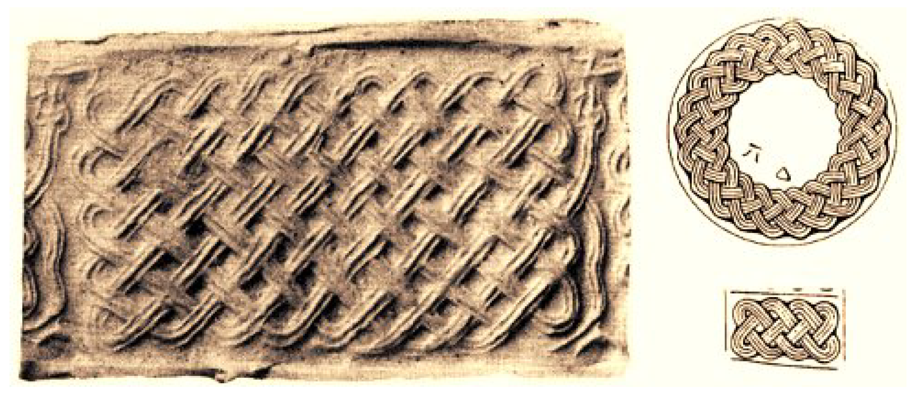
Some of the oldest examples of monolinear curves and knots in rectangular grids associated with them were constructed using plates: Rectangular grids of dimensions , where a, b are coprime numbers. A snake eating its tail, the classical symbol of Ouroboros, the cylinder seal impression from Ur, Mesopotamia, ca. 2600–2500 B.C. showing a snake with interlacing coil placed in nine times five grid (Figure 1) is an example of this construction. Similar examples with plates constructed as rectangular or circular grids are used as stamp seals from Anatolia, ca. 1700 B.C. We assume that stamps, cylinders and seals with knots and links as their motifs appeared before proper writing is invented about 3500 B.C. [1].
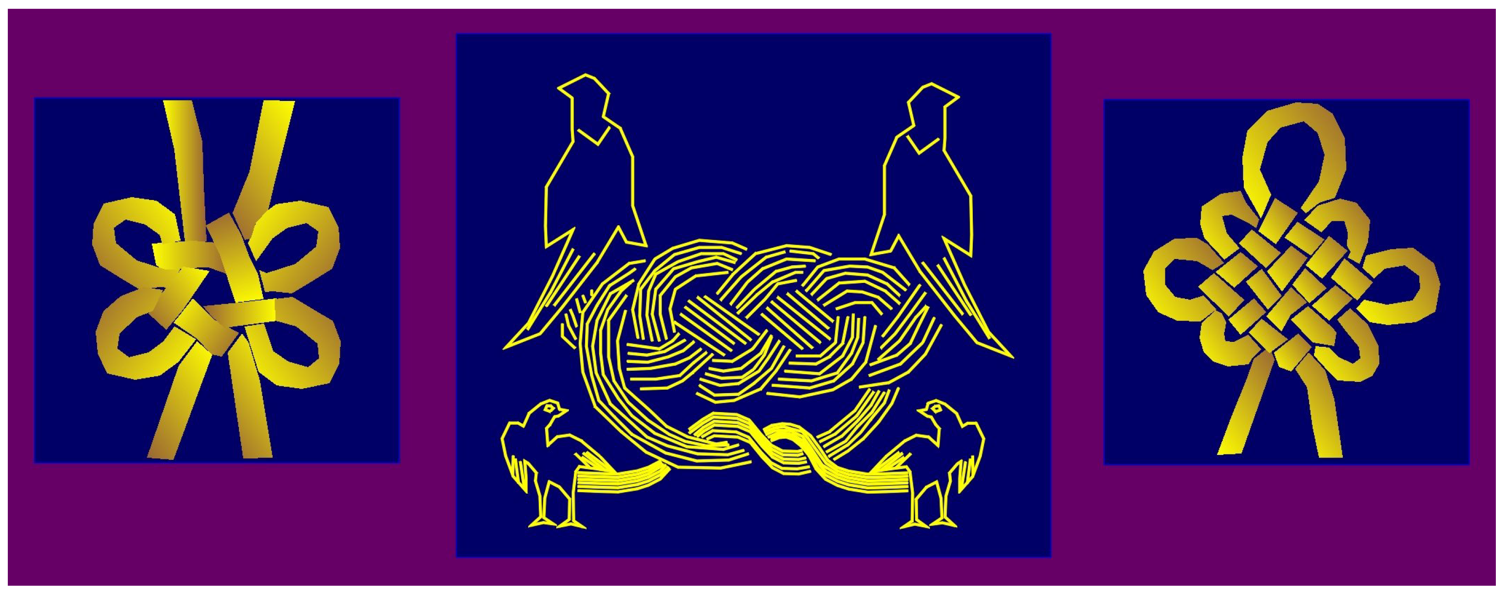
Due to the delicate nature of the medium, few examples of prehistoric Chinese knotting exist today. Some of the earliest evidence of knotting has been preserved on bronze vessels of the Warring States period (481–221 B.C.), Buddhist carvings of the Northern Dynasties period (317–581 A.D.) and on silk paintings during the Western Han period. Chinese knotting is a decorative handicraft art that began as a form of Chinese folk art in the Tang and Song Dynasty (960–1279 A.D.) in China. It was later popularized in the Ming). The art is also referred to as Chinese traditional decorative knots (Figure 2).
Some of the most beautiful legends related to knots appear in Greek mythology. The legend about the Gordian knot, associated with Alexander the Great, is often used as a metaphor for an intractable problem solved by a bold stroke (“cutting the Gordian knot"). Although nobody knows the type of the Gordian knot, the unknotting number, which is one of the simplest knot invariants but also very hard to compute, is also called “the Gordian number".
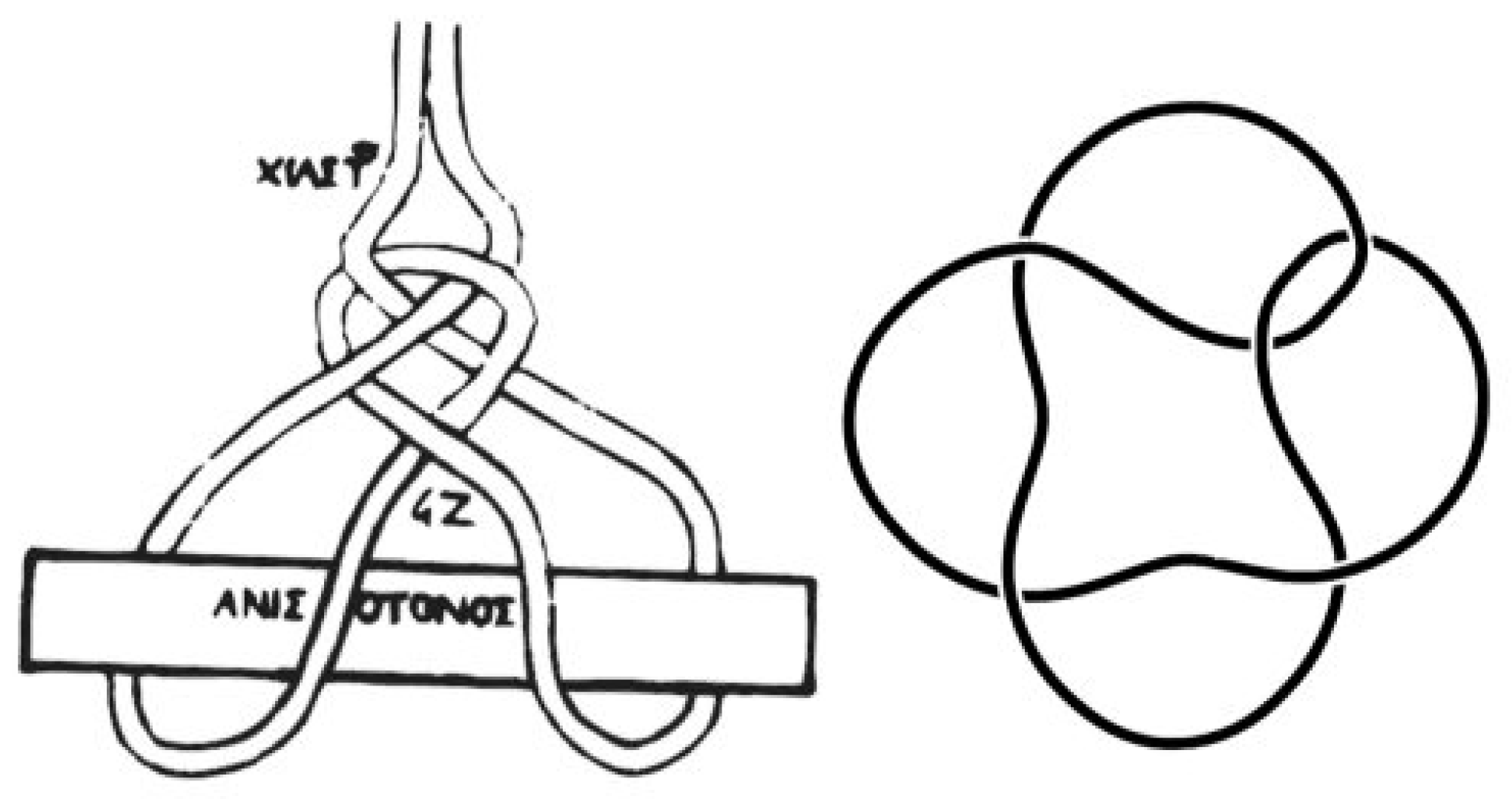
The first study and description of the surgeon’s slings is written by a Greek physician named Heraklas, who lived during the first century A.D. In this essay Heraklas explains, giving step-by-step instructions, eighteen ways to tie orthopedic slings. A closure of each of them represents a knot or link (Figure 3).
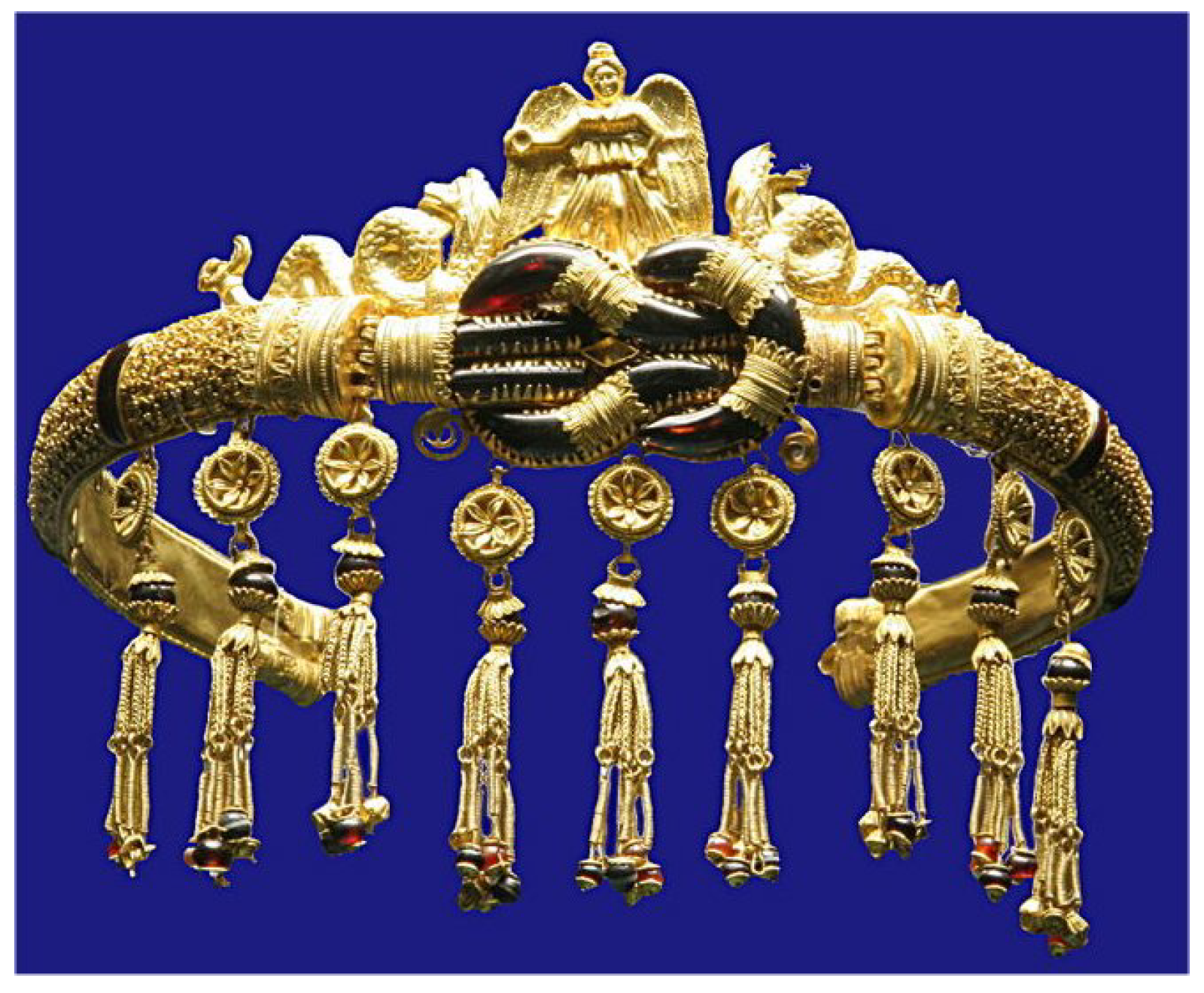
Moreover, wonderful examples of Hercules knots (Figure 4) can be found in the Greek jewelry, beginning from the Minoan period. The reef knot was known to the ancient Greeks as the Hercules knot (Herakleotikon hamma), it was and is still used extensively in medicine as a binding knot. In his Natural History Pliny expresses the belief that wounds heal more quickly when bound with a Hercules knot.
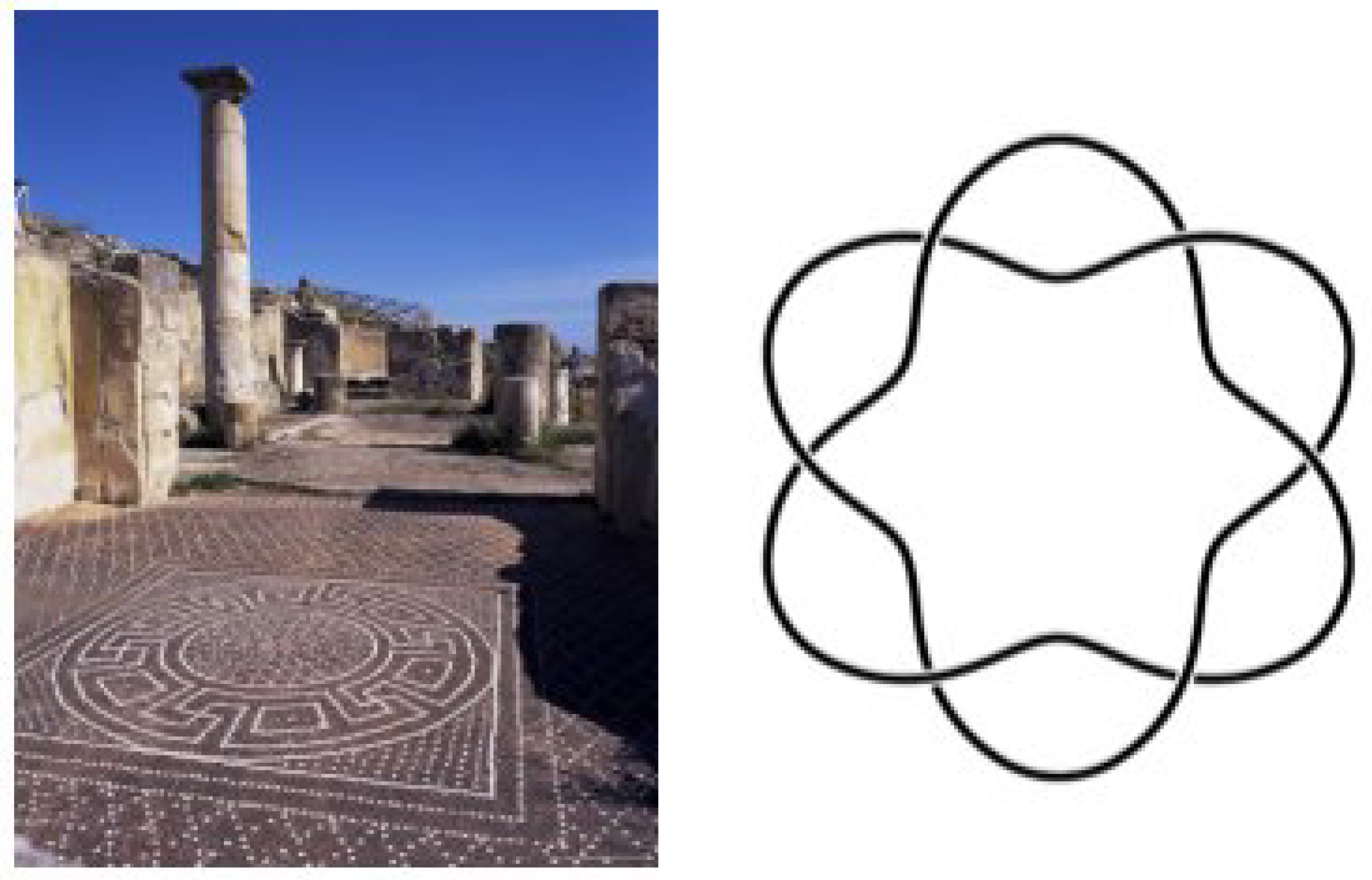
Beautiful examples of knots and links in art can be implicitly found in Greek mosaics. Decorations on Greek floor mosaics in the form of meanders are four-valent graphs that can be thought of as knot projections and easily transformed into the corresponding knots and links by adding the information which strand passes on top of the other. For example, the Greek mosaic (Figure 5a), viewed from knot theory point of view, represents a link (Figure 5b).
2. Mirror Curves
“The imitation of the three-dimensional arts of plaiting, weaving and basketry was the origin of interlaced and knotwork interlaced designs. There are few races that have not used it as a decoration of stone, wood and metal. Interlacing rosettes, friezes and ornaments are to be found in the art of most people surrounding the Mediterranean, the Black and Caspian Seas, Egyptians, Greeks, Romans, Byzantines, Moors, Persians, Turks, Arabs, Syrians, Hebrews and African tribes. Their highlights are Celtic interlacing knotworks, Islamic layered patterns and Moorish floor and wall decorations ” [2].
Celtic knots are one of the highlights of knot-art. Some researchers believe that the root of Celtic knot art is in knot designs in the 10th–11th century eastern mosaics patterns, especially Persian tiling. The very beginning of knotwork art has probably originated in mirror curves constructed from plates, which have been also recognized as the basis of all Celtic knotworks by the antiquarian J. Romilly Allen whose twenty years’ work is summarized in the book Celtic Art in Pagan and Cristian Times [3].
We give a brief outline of the mirror curves construction and details are given in Section 2.3.
Basic construction uses a rectangular grid consisting of squares but can be generalized in two ways: To an arbitrary region of the plane consisting of an edge-to-edge tiling by polygons and by inserting internal two-sided mirrors. First, connect the midpoints of adjacent edges to obtain a 4-regular graph: Every vertex is incident to four edges, called steps. Every closed path in this graph, where each step appears only once, is called a component. A mirror curve is the set of all components. Since the graph is 4-valent, at each vertex we have three choices of edges to continue the path: To choose the left, middle, or right edge. If the middle edge is chosen the vertex is called a crossing. Every mirror curve can be converted into a knotwork design by introducing the relation “over-under”.
The name “mirror curves” can be justified by assuming that all of the outside edges of the region are mirrors, with the additional internal two-sided mirrors placed at the midpoints of all other edges of the polygons, colinear or perpendicular to the edge. For simplicity, assume that we have a rectangular grid consisting of squares, i.e., plate, and that a ray of light is emitted from one edge-midpoint at an angle of . It will travel through the grid and come to the starting point after a series of reflections. If the whole grid was not covered, we can repeat the process by starting at a different edge-midpoint, and continuing until the whole step graph is used, we trace a mirror curve.
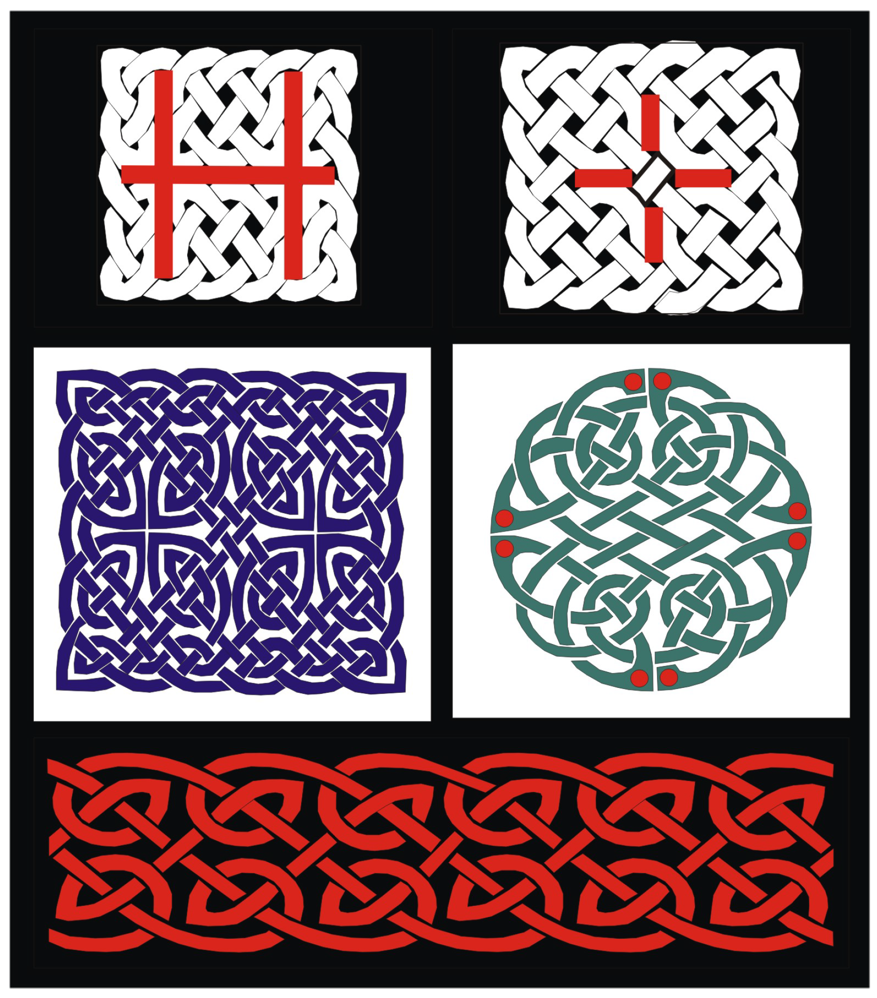
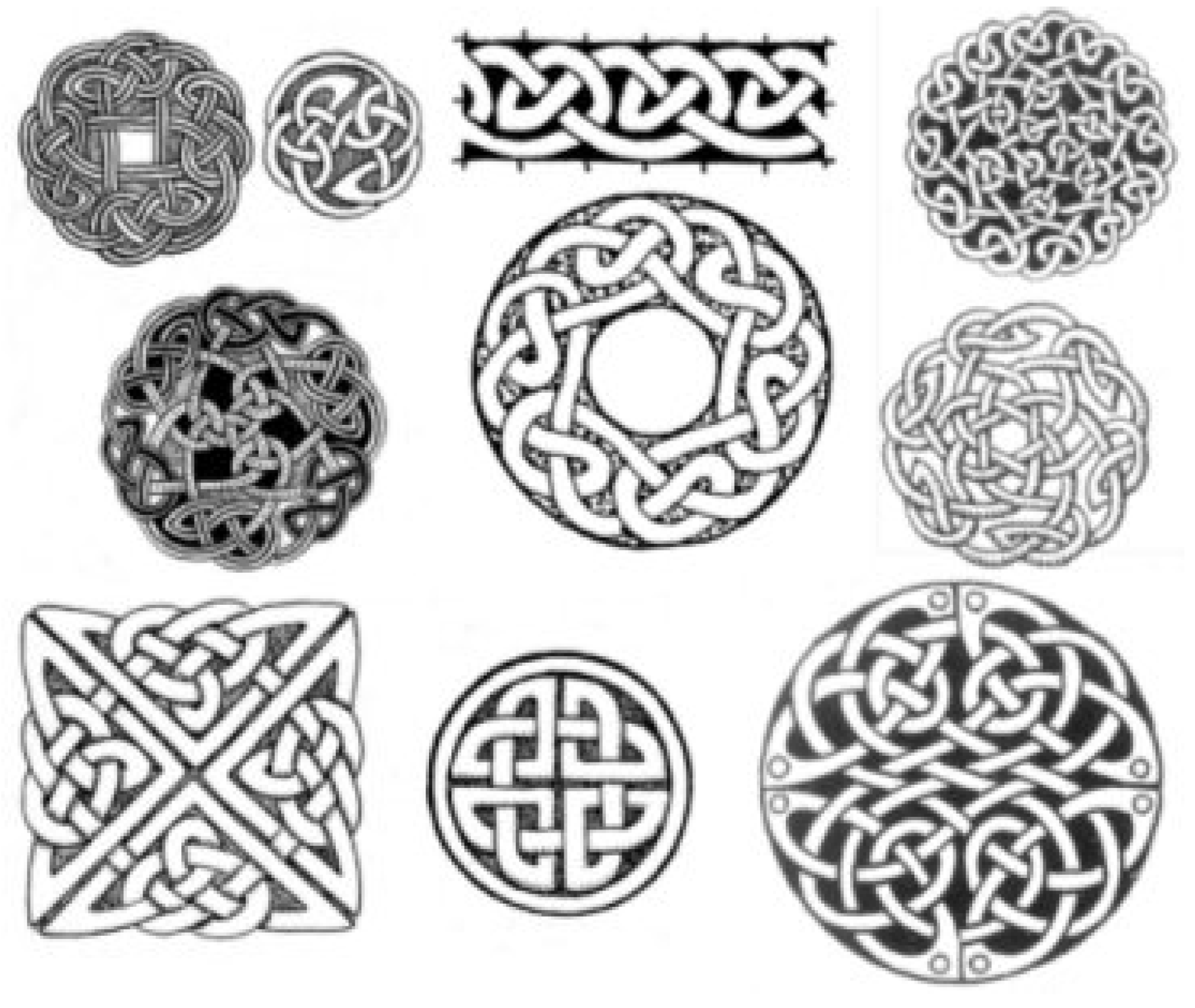
The common geometrical construction principle of these designs, discovered by P. Gerdes, is the use of (two-sided) mirrors incident to the edges of a square, triangular or hexagonal regular plane tiling, or perpendicular to the edges in their midpoints [4,5]. In the ideal case, after the series of consecutive reflections, the ray of light reaches its beginning point, defining a single closed curve. In other cases, the result consists of several closed curves. For example, the following mirror-schemes (Figure 6) correspond to the Celtic designs from G. Bain’s book Celtic Art [2].
The number of mirror curves in a design obtained from plates without internal mirrors is the greatest common divisor of the lengths of plates sides a and b, see Section 2.4. Hence, a single curve, i.e., a knot, is obtained iff a, b are mutually prime numbers. It is interesting that all knots obtained from a single curve on a plate satisfy parametric equations using cos functions known as Lissajous knots [6], and can be reparametrized to be viewed as billiard knots inside of a cube.
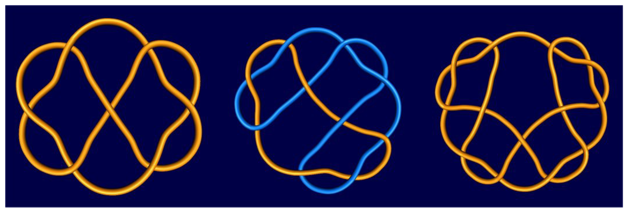
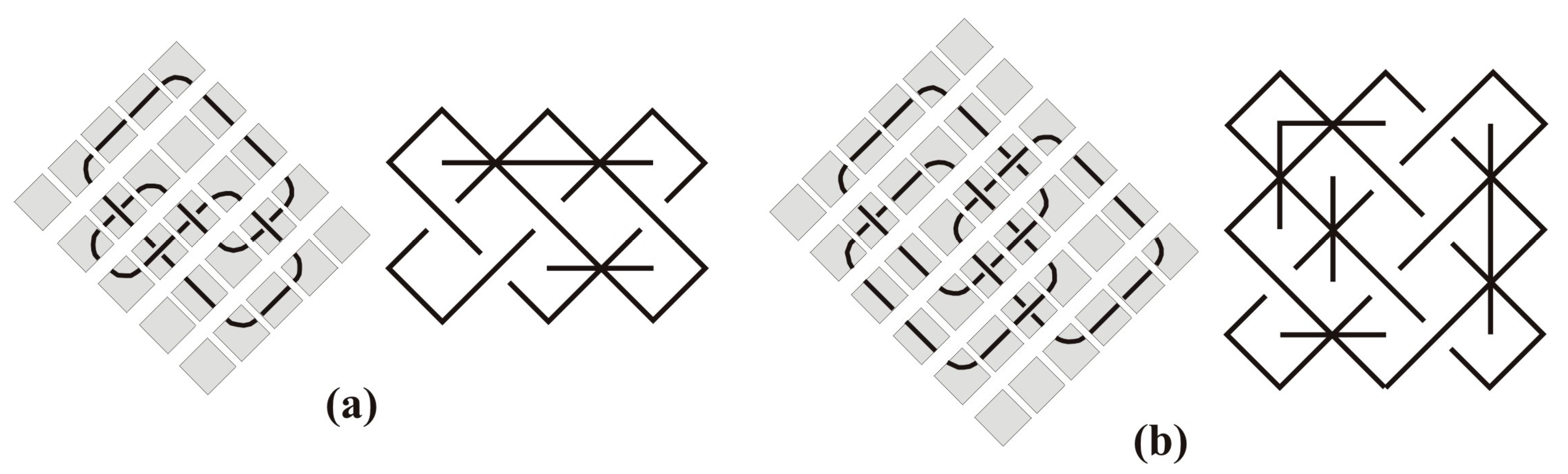
The infinite series of plates, obtained for an arbitrary and , consists of rational knots and links, given by their Conway symbols [7] , , , (Figure 7).
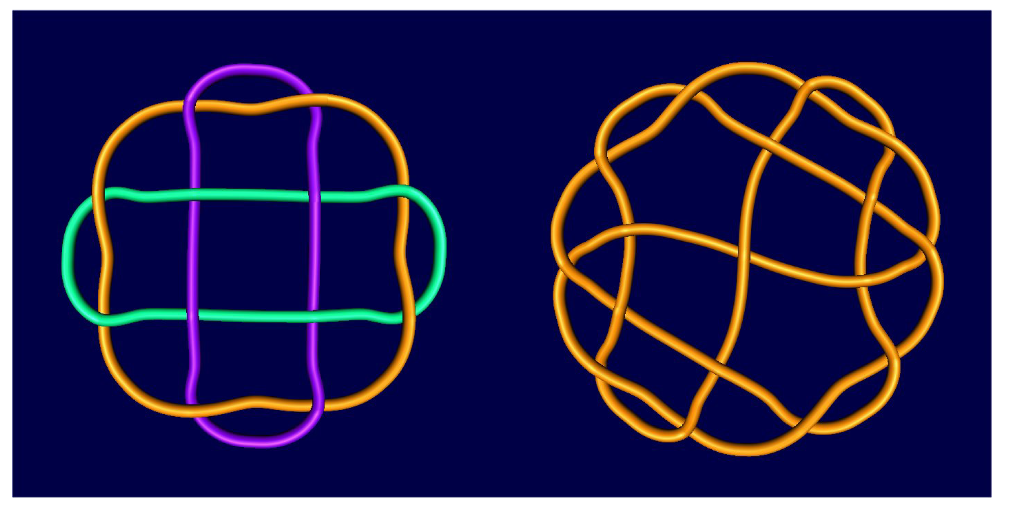
For an arbitrary and we obtain plates with polyhedral knots and links: For we have 3-component link , for the knot , etc. (Figure 8).
2.1. Tamil Threshold Designs
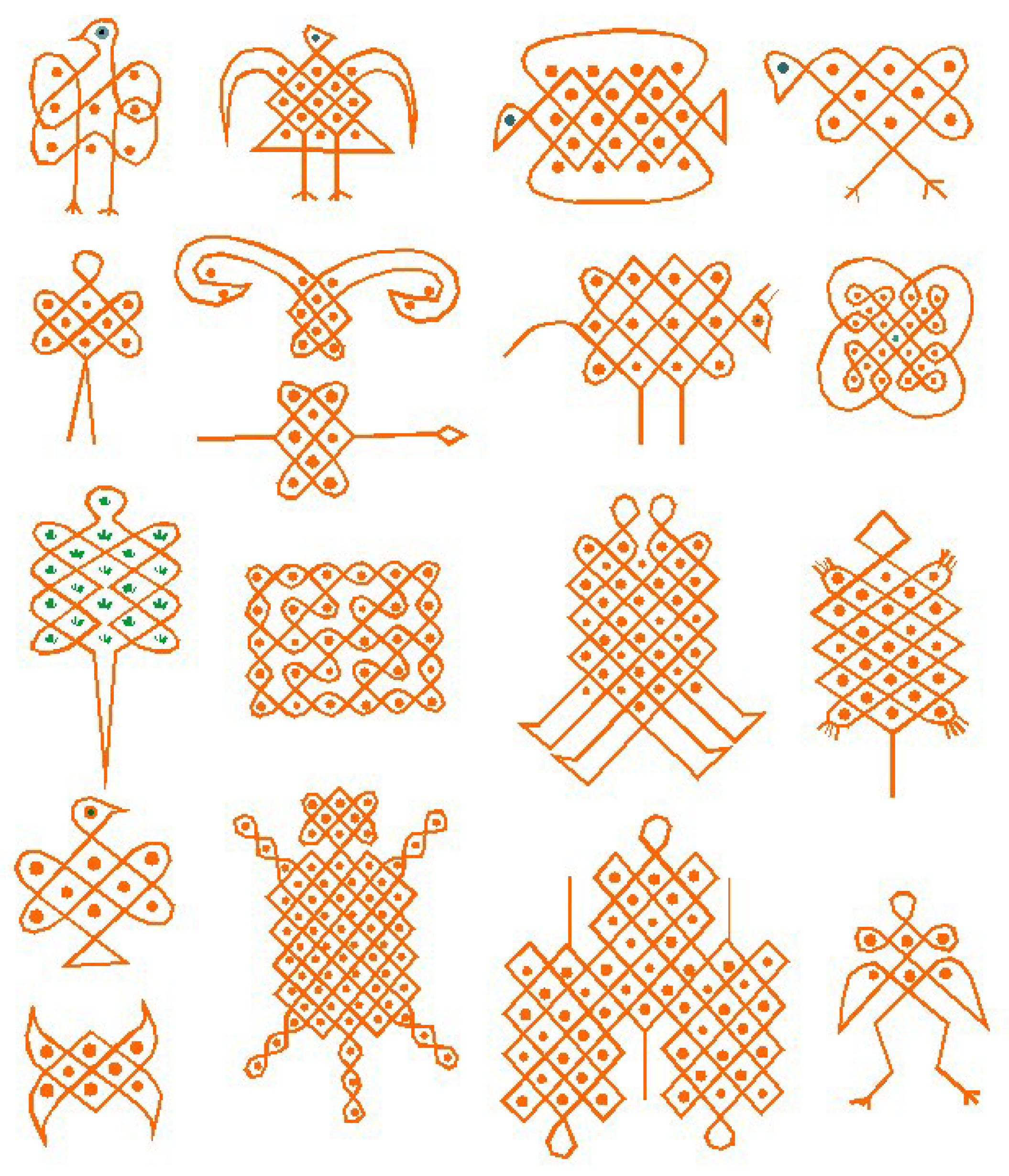
“During the harvest month of Margali (mid-December to mid-January), the Tamil women in South India used to draw designs in front of the thresholds of their houses every morning. Margali is the month in which all kinds of epidemics were supposed to occur. Their designs serve the purpose of appeasing the god Siva who presides over Margali. In order to prepare their drawings, the women sweep a small patch of about a yard square and sprinkle it with water or smear it with cow-dung. On the clean, damp surface they set out a rectangular reference frame of equidistant dots. Then the curve(s) forming the design is (are) made by holding rice-flour between the fingers and, by a slight movement of them, letting it fall out in a closed, smooth line, as the hand is moved in the desired directions. The curves are drawn in such a way that they surround the dots without touching them” [8].
The ideal design according to Tamil culture is composed of a single continuous line. Names given to designs formed of a single “never-ending” line are normally pavitram, meaning “ring” and Brahma-mudi or “Brahma’s knot” (Figure 9). The purpose of the pavitram is to scare giants, evil spirits, or devils away.
2.2. Tchokwe Sand Drawings
“The Tchokwe people of northeast Angola are well known for their beautiful decorative art. When they meet, they illustrate their conversations by drawings on the ground. Most of these drawings belong to a long tradition. They refer to proverbs, fables, games, riddles, etc. and play an important role in the transmission of knowledge from one generation to the other” [9].
“…Just like the Tamils of South India, the Tchokwe people invented a similar mnemonic device to facilitate the memorization of their standardized drawings. After cleaning and smoothing the ground, they first set out with their fingertips an orthogonal net of equidistant points. The number of rows and columns depends on the motif to be represented. Applying their method, the Tchokwe drawing experts reduce the memorization of a whole design to that of mostly two numbers and a geometric algorithm. Most of their drawings display bilateral and/or rotational ( or ) symmetries. The symmetry of their pictograms facilitates the execution of a drawing. This is important, as the drawings have to be executed smoothly and continuously. Any hesitation or stopping on the part of the drawer is interpreted by the audience as an imperfection and lack of knowledge, and assented with an ironic smile” [9].
Tchokwe sand drawings (Figure 10) called sona (singular: lusona) played an important role in transmitting knowledge and wisdom from one generation to the next. Young boys enjoyed making sand drawings with their fingers and hearing stories about them. They have learned how to make simple drawings and their meaning during the period of intensive schooling, the mukanda initiation rites. More complicated sona were only known by the story tellers, who were real akwa kuta sona (those who know how to draw), highly esteemed and forming a part of an elite in Tchokwe society [4].
2.3. Construction of Mirror-Curves
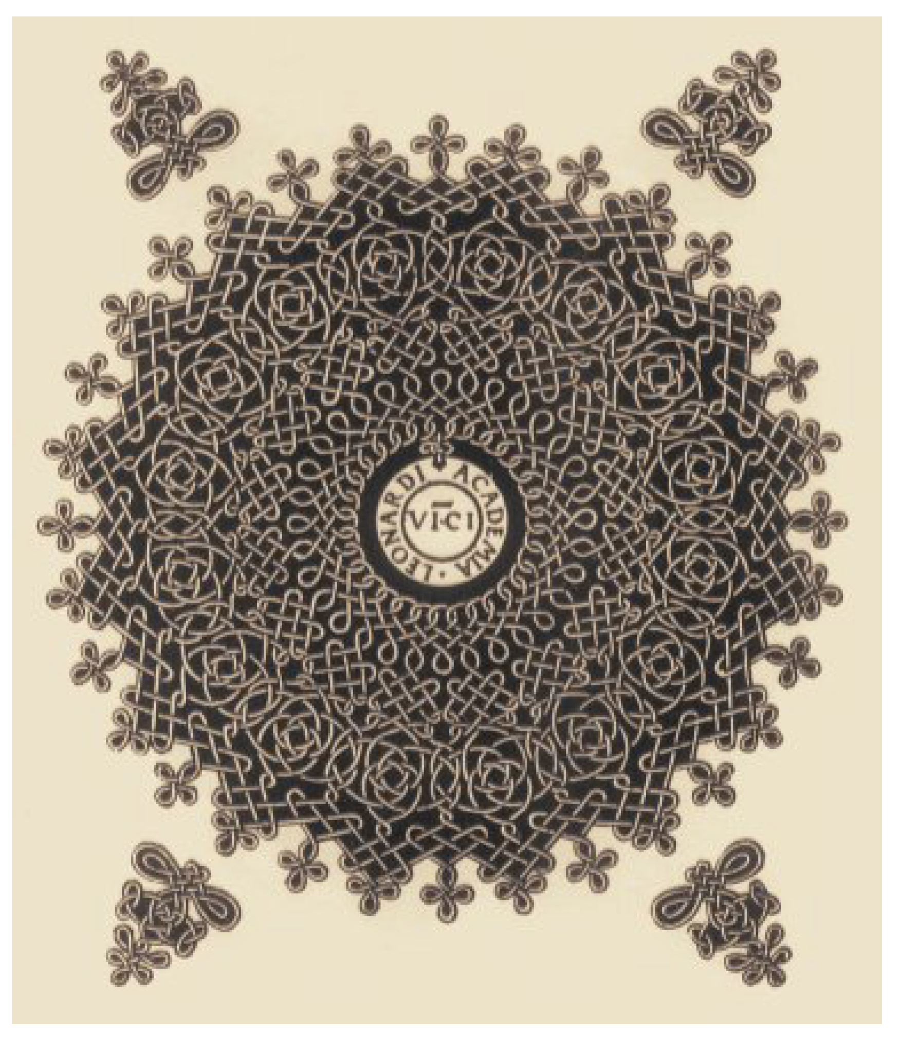
“Leonardo spent much time in making a regular design of a series of knots so that the cord may be traced from one end to the other, the whole filling a round space…” [2].
Leonardo and Dürer, two of the greatest painters-mathematicians, were interested in constructing knot designs, closely related to mirror curves [2] (Figure 11). They knew and very effectively used the fact that for a rectangular square grid of dimensions a, b, where a and b are relatively prime, mirror curve is always a single closed curve uniformly covering the rectangle.
The common geometrical construction principle of Celtic, Tchokwe, or Tamil knot designs, elaborated by P. Gerdes, is the use of (two-sided) mirrors incident to the edges of a square, triangular or hexagonal regular plane tiling, or perpendicular to the edges in their midpoints [4,5,8,9]. In the ideal case, after the series of consecutive reflections, the ray of light reaches its beginning point, defining a single closed curve. In other cases, the result consists of several closed curves. For example, the following mirror-schemes (Figure 6) correspond to the Celtic designs from G. Bain’s book Celtic Art [2].
Gerdes’ books [10,11] present examples and analysis of mirror curves in Ancient Egypt, Mesopotamia, India and African cultures, and [12,13] present an analysis of the relationship between mirror curves and matrices.
Moreover, there is one more beautiful geometrical property: Mirror curves can be obtained using only a few different prototiles. In particular, only three prototiles are sufficient for construction of all mirror curves with internal mirrors incident to the cell-edges of a regular triangular tiling, five for square, and 11 for hexagonal regular tiling (Figure 12) [14].
Using the combinations of polygons from 11 uniform Archimedean tilings [15], or prototiles producing an impression of space structures and colored prototiles, we may obtain artistic interlacing patterns, examples of modular design: The use of a few initial elements (modules-prototiles) for creating an infinite collection of designs. The mirror curves obtained from Archimedean tilings resemble the optical phenomenon: Change in direction of a light ray which transfers from one to the other physical environment.
As we already stated, the ideal mirror curve was a monolinear one, consisting of a single curve and corresponding to a knot. Monolinear curves can be obtained from k curves, covering a region of a plane tiling denoted by T by placing internal mirrors keeping in mind the effect it has on the curve. These moves are sometimes referred to as the “curve surgery”:
- Mixed crossing
- Any mirror placed in a crossing point of two distinct curves connects them into one curve;
- Self-crossing
- Depending on its position, a mirror placed into a self-crossing point of an (oriented) curve either preserves the number of curves, or breaks the curve in two (Figure 13).
Starting with k curves the minimal number of mirrors needed to transform them into a single curve is and they need to be added in mixed crossing. This simple algorithm is obviously finite. If , we have a single mirror curve, so no additional two-sided mirrors are needed. If the number of components is k (), we place first two-sided mirror in the crossing of two different curves, connect them and obtain components. Continuing in the same way, a single mirror curve will be obtained after introducing mirrors. Our game becomes more interesting if we allow adding mirrors in self-crossing points of the same component. This move can either preserve the number of curves or increase it by 1, so we can end up with a single or multi-component curve.
In the special case of a rectangular square grid of dimensions a, b, the initial number of curves obtained without internal mirrors is equal to the greatest common divisor , so in addition to the minimal number of mirrors needed to obtain a single curve, we know the maximal number . In general, we can use these rules to modify any monolinear mirror curve without increasing the number of components (Figure 14).
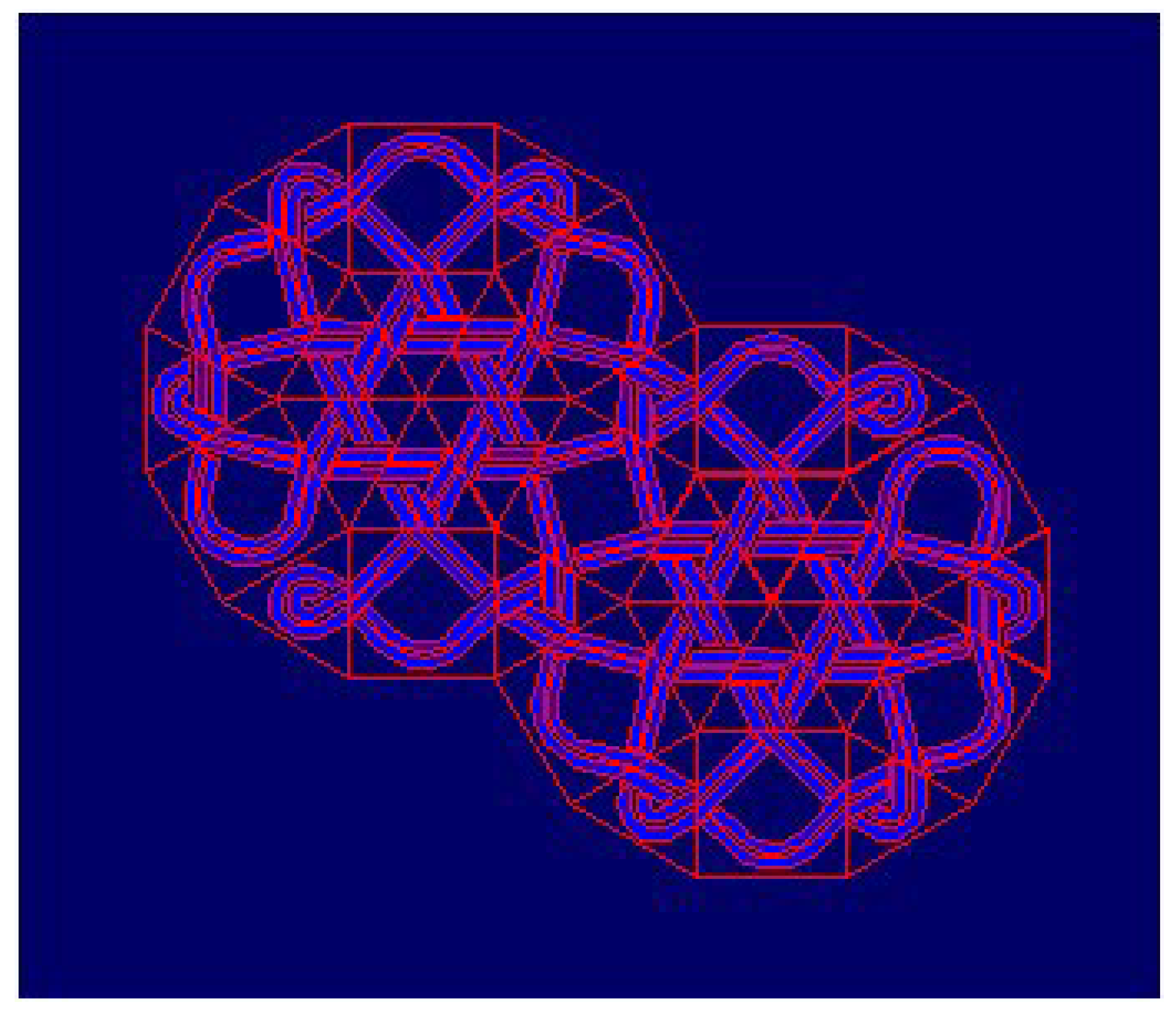
Notice that the construction of mirror curves is independent from the metric properties or the geometry of the surface, so the same construction principle can be applied to any edge-to-edge tiling of an arbitrary surface, say sphere or a hyperbolic plane. Using the rules for adding two-sided mirrors, any mirror curve can be converted in a single mirror curve in a finite number of steps (Figure 15), as we have described above for plane tilings.
2.4. Combinations of Mirror-Curves
Let us now describe four general rules for combining plate designs and/or mirror curves. The first three rules are given by P. Gerdes [5], and the fourth is proposed by S. Jablan. We will restrict our attention to mirror curves obtained from polyominoes with congruent square cells.
Construction rules:
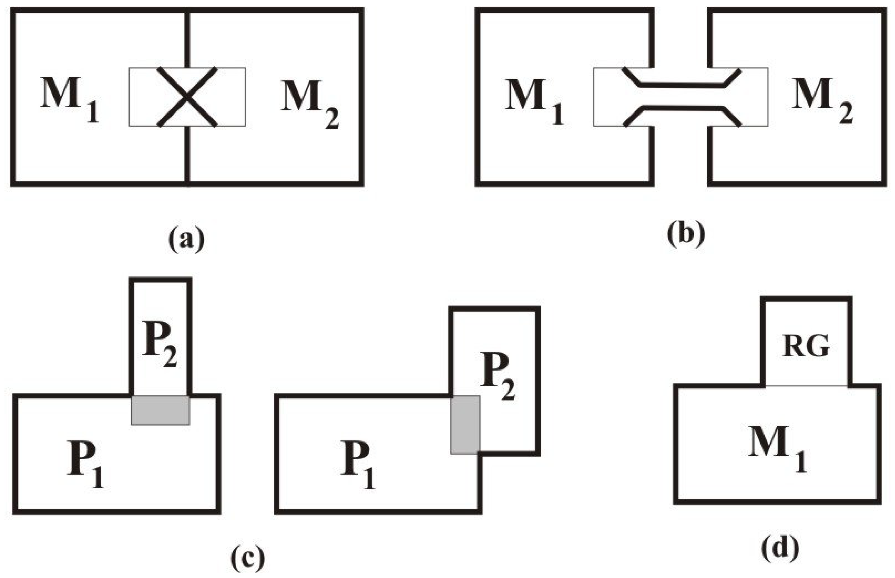
- The first rule describes how to combine two mirror curves that share one edge of an open cell on their borders (Figure 16a). Such a composition corresponds to the direct product of s, and it was probably one of the most exploited constructions in knotwork art. For given mirror curves and , we will call this kind of direct product ×-direct product and denote it by . If we combine two mirror curves in this way, first with , and the other with components, the result is a new mirror curve with components. Hence, the ×-direct product of two 1-component mirror curves is a new 1-component mirror curve. This idea was used, for example, in the Tchokwe designs and in many Celtic friezes.As a particular application of the first rule, we can add a single square to the border of any monolinear mirror curve. This transformation corresponds to adding an external loop to a diagram. It does not change the number of components and can be repeated, since it has a decorative function in knotwork art. For example, the Tamil (unknot) design from Figure 9a is created by a series of external loop additions, beginning from the ; the knot design from Figure 9b by adding loops to the ; and the knot design from Figure 9c by adding loops to the . The same construction is used for Tchokwe designs (Figure 10a).
- The second rule is the one defining the direct sum in knot theory (Figure 16b) (Notice that the first and second rule, i.e., ×- and -product of mirror curves both correspond to the direct product of knots , but the first with a nugatory crossing. Knots or links obtained by using ×- and -product of mirror curves are ambient isotopic to , but not mutually isomorphic as knot or link diagrams.) In the language of mirror curves and , it means that we cut one external edge of each mirror-curve and , and reconnect them again to obtain a new mirror-curve that will be denoted by .
- The third rule is restricted to plate designs: Two monolinear plate designs whose overlap consists of exactly two cells will give a new monolinear plate design. The schematic interpretation of the third rule is given in Figure 16c.
- Adding plate design to plate design is an edge-to-edge identification of their border cells belonging to rectilinear borders (Figure 16d). In the same way, we can add a plate design to some mirror curve M placed in some polyomino. This operation can be generalized to adding plate designs to polyominoes.The fourth rule tells us that adding any design in a grid , such that to any monolinear mirror curve M (or monolinear plate design ) along the edge b, produces a monolinear design (Figure 16d). In particular, any square added to a monolinear design gives a new monolinear design.
Moreover, adding a mirror curve to a monolinear mirror curve so that every curve contact point along edge b of the polyomino in which is placed belongs to a different component of . The new mirror curve will produce a monolinear curve.
These four rules are sufficient for creating monolinear plate designs and extend the monolinearity from s to plate designs. Additional sophistication and variety comes from adding internal mirrors, illustrated in Figure 13. Symmetric mirror curves prevail in the knotwork art since symmetry is regarded as desirable visual property. This means that most of the mirror arrangements are not aesthetically pleasing: For example, only 8 out of 52 two-mirror arrangements from are symmetrical.
We propose the following method for constructing symmetric mirror curves from a symmetric monolinear plate design P. First place an internal mirror in some crossing A of P and trace an oriented mirror curve M. Now we have two possibilities:
- if our mirror curve M does not cover P completely, choose a mixed crossing point on M, symmetric to A and put a mirror symmetric to the mirror in A (Figure 17a). If a symmetric point with this property does not exist, rotate the mirror in A for around its midpoint and then place the mirror symmetric to it (Figure 17a);
This approach is used to explain the construction of different mirror curves occurring in Tamil, Tchokwe and Celtic knotworks. We already explained and illustrated knotwork designs that obtained from a single monolinear plate design by adding a series of external loops, as well as designs obtained as direct products of monolinear plate designs (Rule 1, denoted by ×).
The first rule, ×-direct product, is very frequently used in Celtic knotwork art for the construction of friezes (or bordures), as well as the ‖-direct product (Rule 2). Both of them are the standard tools for obtaining translational repetitive structures: Friezes or even plane symmetry groups.
Applying the second rule connects two monolinear s at their corners, i.e., it is the ‖-direct sum of the corresponding knots. Similar approach would be using (more or less) “open” plate designs s and the ‖-direct sum of the corresponding mirror curves. Although resulting composite knots and links will be the same, obtained patterns will be visually very different.
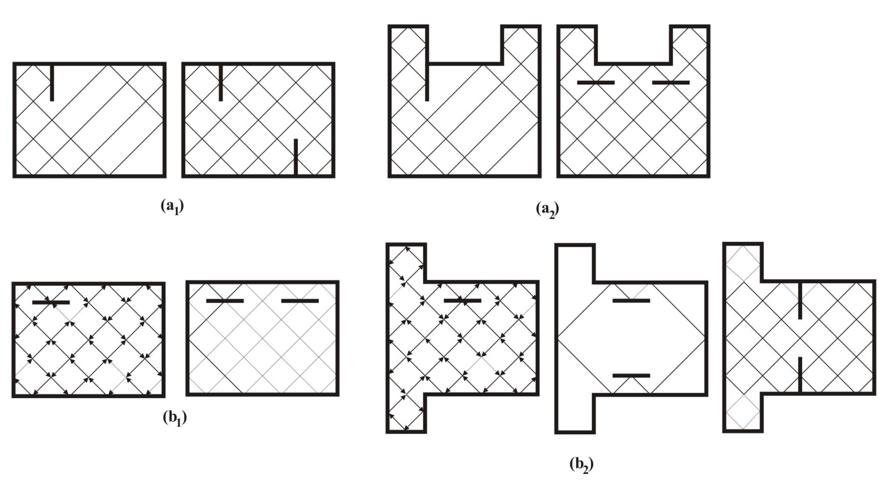
In order to analyze Celtic knotworks based on ‖-direct product first we need to insert some internal mirrors perpendicular to the edges in basic (monolinear) s, in order to obtain parts or “tangles” of Celtic knotworks with an appropriate placement of incoming and outgoing strands. The possible choices for their positions are two top (or bottom) corners of an elementary , two diagonal (ascending or descending) corners, or all four corners forming a tangle. In the first case we place internal mirrors perpendicular to “vertical” and “horizontal” edges of border cells, forming an L-shape form. Furthermore, cutting the long edge(s) of the design and reconnecting them, we obtain different frieze designs (direct products of basic s) with incoming and outgoing strands appropriately placed (Figure 18).
Another possibility is creating “tangles” from s (Figure 18) and composing them into chains (or closed circles) (Figure 19 and Figure 20). In the case of Tchokwe sand drawings a similar strategy was used in order to obtain “open” s that can be further composed by ‖-direct sum or ×-direct product (Figure 10b) to form larger knotworks.
The third rule was one of the favorite rules in the construction of Tchokwe sand drawings. A whole series of “social” monolinear plate designs representing a leopard with cubs, a design called kambava wamulivwe that represents an animal called kambava that died inside a rock (Figure 21b), or lusona drawing called tambwe that represents a lion (Figure 21c) are composed in this way.
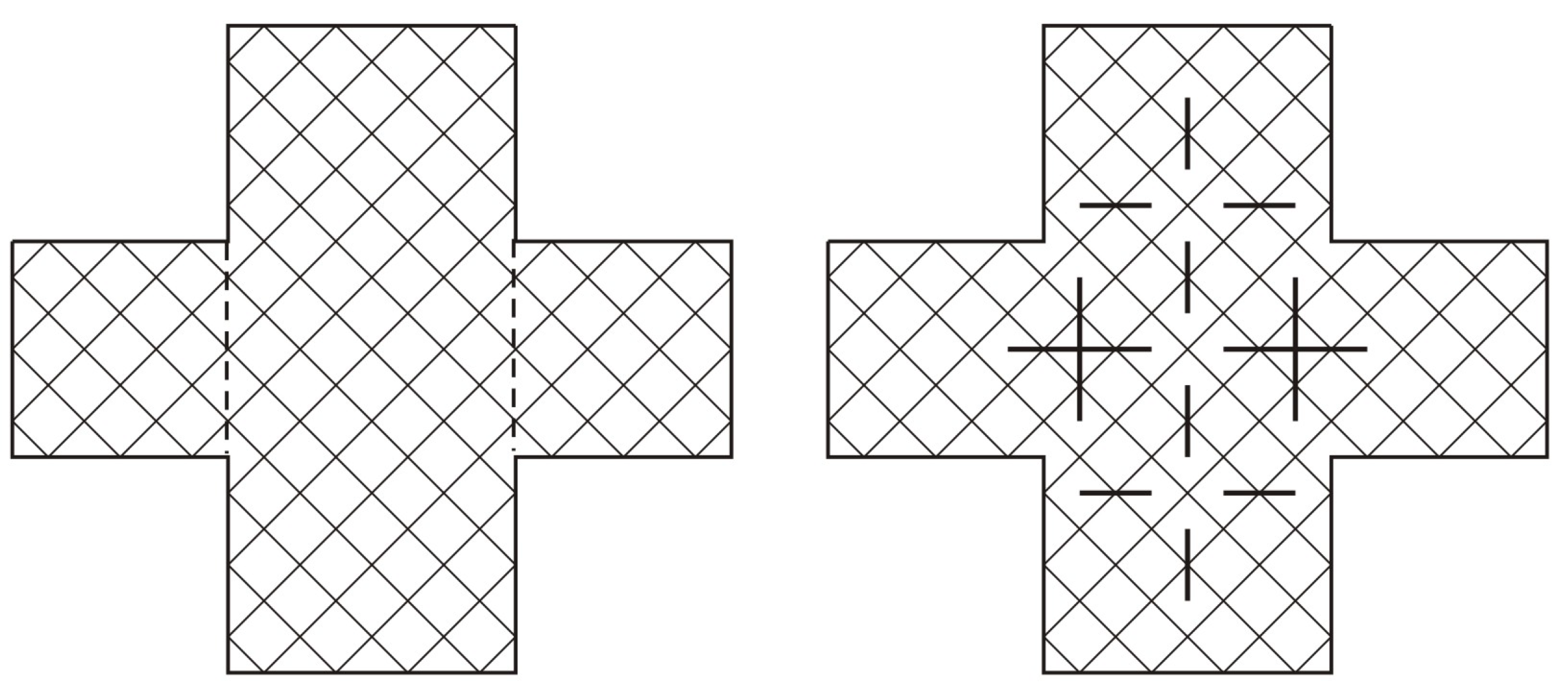
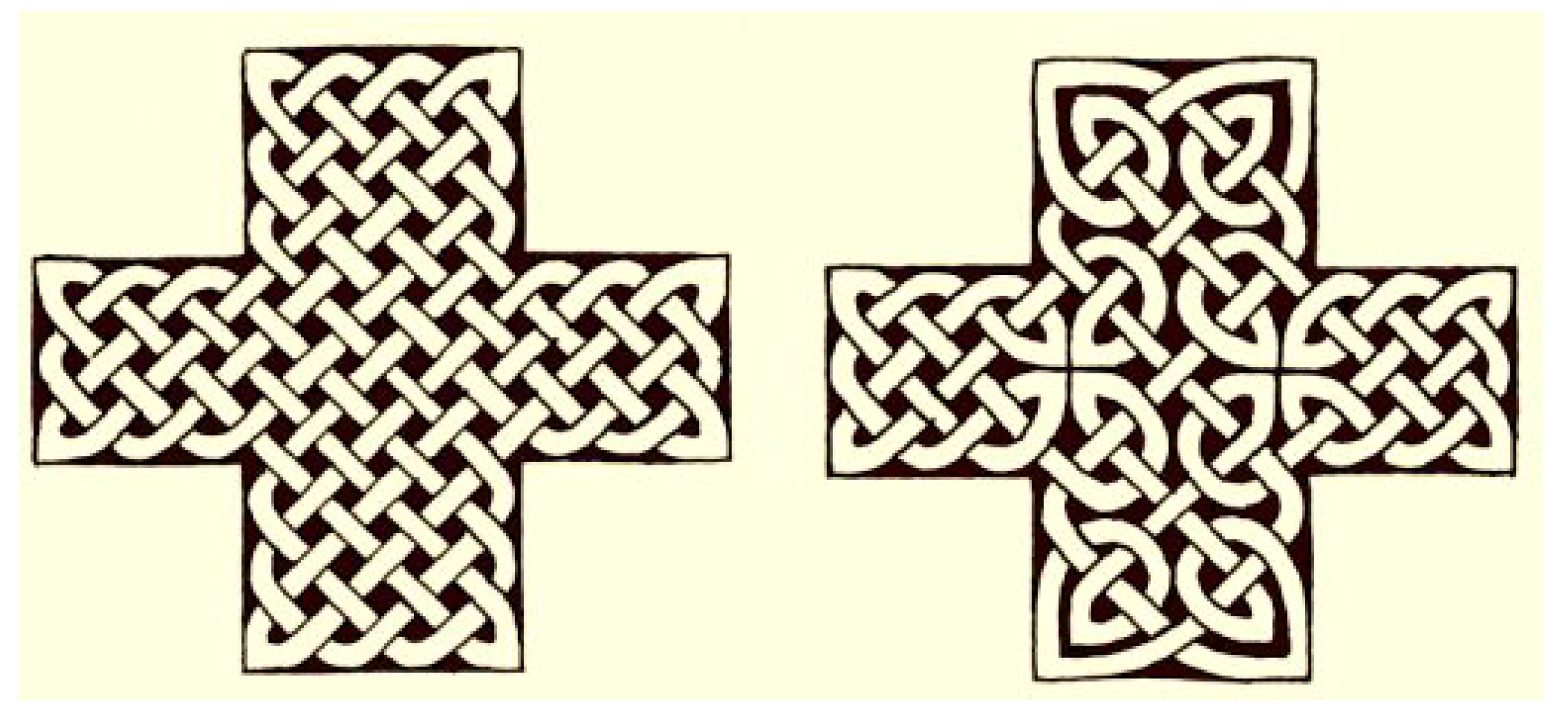
The fourth rule offers the highest degree of freedom with respect to the shape of the plate, often producing symmetric plates in knotwork art (Figure 22). Hence, we can construct a perfect monolinear curves in any shape obtained by adding different plates.
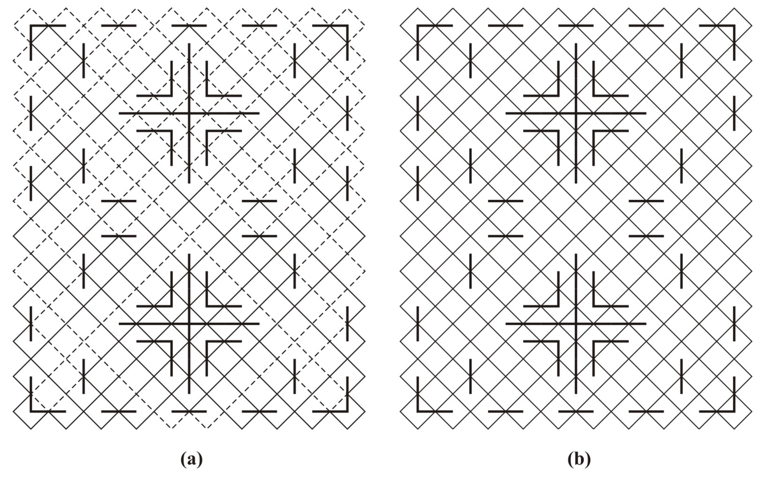
Creating a variety of monolinear plate designs opens the door to artistic creativity and play: There is a huge number of ways for introducing internal edge-incident and edge-perpendicular mirrors while preserving monolinearity (Figure 23, Figure 24, Figure 25 and Figure 26).
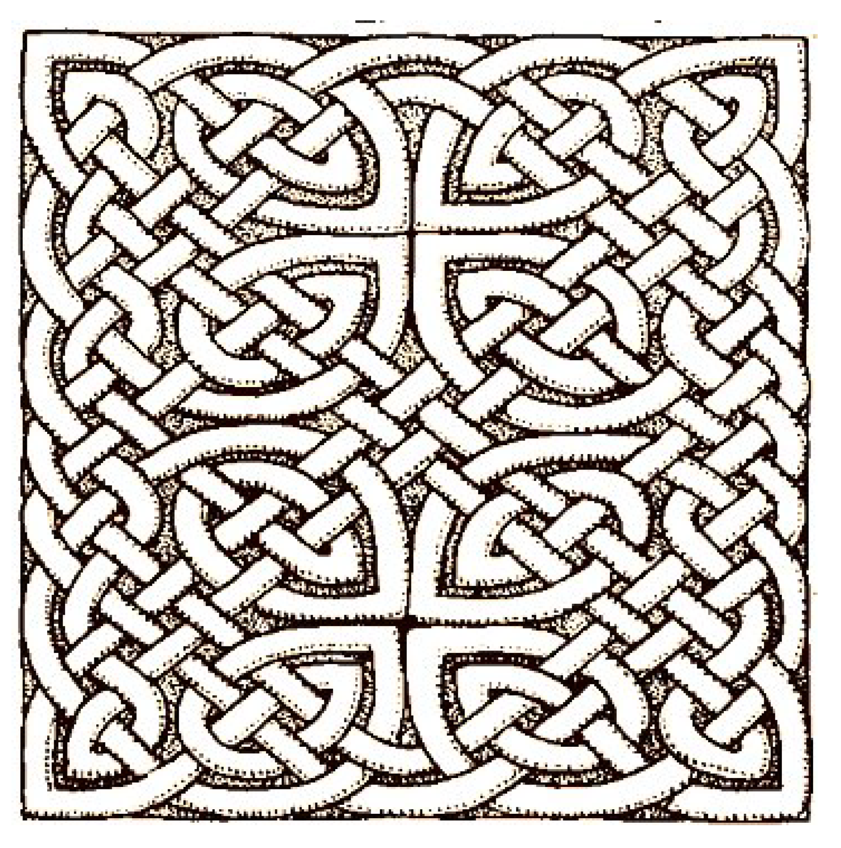
Together with the remarkable example of a monolinear cross knot design (Figure 23), interesting examples of a complex monolinear design are shown in Figure 25 and Figure 26. Because the symmetric version of the same design (Figure 26a) is a two-component knot design, the Celtic master modified it into an almost symmetric monolinear design by breaking symmetry (Figure 26b).
3. Symmetry and Classification of Knotwork Designs
P. Cromwell [16] used symmetry of mirror curves for the classification of the Celtic frieze designs, and P. Gerdes [8] for the reconstruction of Tamil designs. At the first glance it seems that symmetry is the mathematical basis for the construction and possible classification of perfect curves [8,14,16], but the existence of asymmetric curves asks for alternative approaches.
If we treat them as purely geometric object we can impose the following equality relation:
Two mirror curves are equal iff there is a similarity transforming one into the other.
In other words, if one mirror curve can be obtained from the other by a combined action of proportionality and isometry, they are considered to be the same. This relation can be studied on the level of mirror arrangements, in a very similar way.
A transformation S of the Euclidean n-dimensional space is called isometry if for every two points X, Y and their images , holds .
A figure f is any non-empty subset of points of space.
A figure is called invariant with regard to a transformation S if , and S is called a symmetry of f.
Symmetries of a figure f form a group called the symmetry group of f and denoted (see, e.g., [15,17,18]).
Isometric symmetry groups of the space can be classified according to a sequence of maximal proper (sub)spaces invariant with respect to the action of transformations of the groups in question. Symmetry groups of friezes , bands , plane ornaments , and layers can be used for the classification of knot-work patterns. Isometric symmetry groups will be denoted according to the crystallographic notation (or Hermann and Maugin notation).
There exist exactly 7 symmetry symmetry groups of friezes, 31 symmetry groups of bands, 17 symmetry groups of plane ornaments, and 80 symmetry groups of layers (see, e.g., [15,17,18,19,20]).
The fundamental region of a symmetry group of an object or pattern is the smallest part of the pattern, which, based on the symmetry, determines the whole object or pattern.
In all symmetry-oriented classifications of interlaced patterns, i.e., infinite knotwork patterns (e.g., [16] or in [15]), symmetry is used as the only criterion for the classification. Linear knotwork patterns are classified according to 7 symmetry groups of friezes, or 31 symmetry groups of bands [15,19,21] without taking into account their topological or knot-theoretical properties. In the same way, plane symmetry patterns are classified according to 17 symmetry groups of ornaments or 80 symmetry groups of layers. In all these cases we have an asymmetric fundamental region multiplied by symmetries belonging to the symmetry group, without taking into consideration that the fundamental region can be any asymmetric tangle with its particular knot-theoretical properties. For example, according to the symmetry oriented classification, two bands shown in Figure 27 will be considered as equivalent because their symmetry group is p1a1, in spite of the fact that the first is based on the tangle giving as the numerator closure Hopf link (2), and the other is the direct product of knots .
For the classification of infinite symmetric interlaced patterns we propose the following two criteria:
- isometric symmetry group of the pattern;
- tangle inscribed in the fundamental region.
These criteria are not always sufficient, and we also need to consider other knot-theoretical properties such as whether a pattern represents prime or composite arrangement.
As in the case of an n-tangle () in general, we may consider all possible closures of tangles contained in the fundamental region as a base for further classification. For example, by joining left and right ends of the tangles (Figure 28) that are the basic elements of two friezes with the same symmetry p121 we obtain links and , respectively.
This classification, proposed by S. Jablan and Lj. Radović in 2001, is similar to the approach proposed earlier by I. Emery [22].
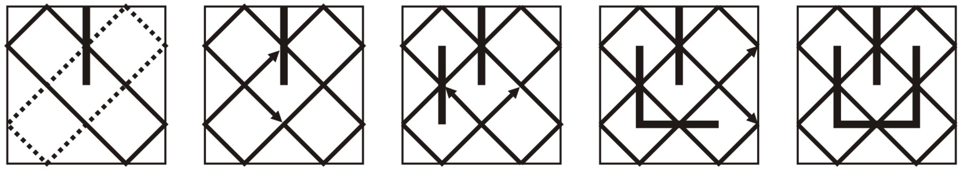
4. Knot Mosaics and Mirror Curves
Modularity is very effectively and widely used in the history of ornamental art [18]. It is a manifestation of the principle of economy or simply the optimization problem of how to minimize the number of basic elements (modules) while maximizing the number of different ornaments (structures) obtained by their recombination. A typical example of modular elements are prototiles for different tilings, e.g., a Truchet tile or “kites” and “darts” as the basic elements of Penrose tilings. A lesser known fact is that knot tilings are also modular: Five types of basic elements in a regular square grid are sufficient to construct shadows of all possible knots and links. A set of such elements named KnotTiles (Figure 29) is proposed by the first author [23], and a similar set is produced by R. Fathauer [24]. The second set of elements is used by S. Lomonaco and L. Kauffman to construct knot mosaics and discuss their connection with quantum computing [25]. The Lomonaco–Kauffman Conjecture that knot mosaics are equivalent to the tame knot theory is proved by T. Kyria [26] (Figure 30 and Figure 31). In his book Knots: Mathematics with a Twist [27] A. Sossinsky noticed that smoothings of crossings, effectively used in skein relations for computing knot polynomials and for obtaining Kauffman states of knots and links, are nothing else than the placements of two-sided mirrors in mirror-curves, used by Celtic knot masters to construct knots decorating their burial stones, menhirs, or illuminations in manuscripts. In Mirror-curves and Knot Mosaics [28] we show the equivalence of knot mosaics, mirror curves, and grid (arc) representations of knots and links. Moreover, we introduce codes for mirror-curves suitable for computer applications, and use them for computation the Kauffman bracket polynomial and L-polynomial of knots and links.
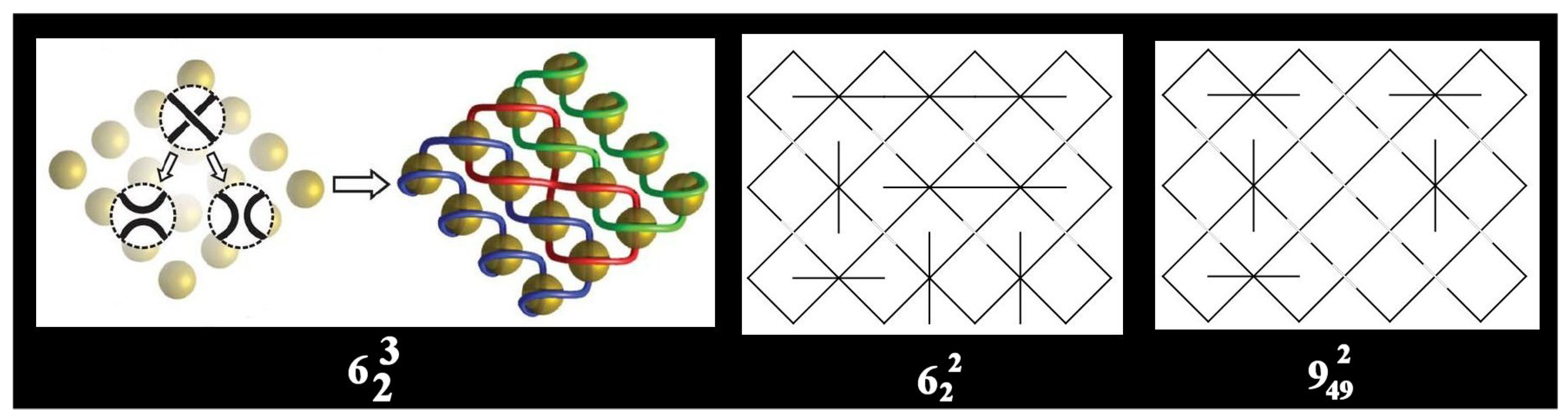
The scientific relevance of mirror curves has been most recently confirmed in physics paper Reconfigurable Knots and Links in Chiral Nematic Colloids [29] (Figure 32). The authors describe a method for configuring so-called Saturn rings (single defect loops around colloid particles) in nematic colloids using laser tweezers. This control over the configurations of the Saturn rings allows them to classify all nematic braids in a colloidal array, and all knots and links obtained in the particle array. Knots and links obtained in this way represent a special class of mirror-curves, containing only positive crossing that correspond to the particles. The authors have synthesized several examples like the Hopf link, trefoil and the Borromean rings, but then managed to distinguish almost 40 different knot and link types (with the links and omitted) supported in the . They conclude that such a large diversity of topological objects suggests that it is possible to design any knot or link on a sufficiently large colloidal array. In the attempt to extend these results we generate all knots and links from arrays of dimensions for , satisfying specific conditions mentioned above. We distinguish more than 1000 of different knot and link types. However, we are still not able to prove that all knots and links can be realized as the mirror-curves satisfying the mentioned specific requirements on crossings and matrix columns, although we know that mirror-curves are equivalent to the tame knot theory, i.e., all knots and links can be realized as mirror-curves in a sufficiently large grid.
5. Knots in Modern Sculpture and Architecture
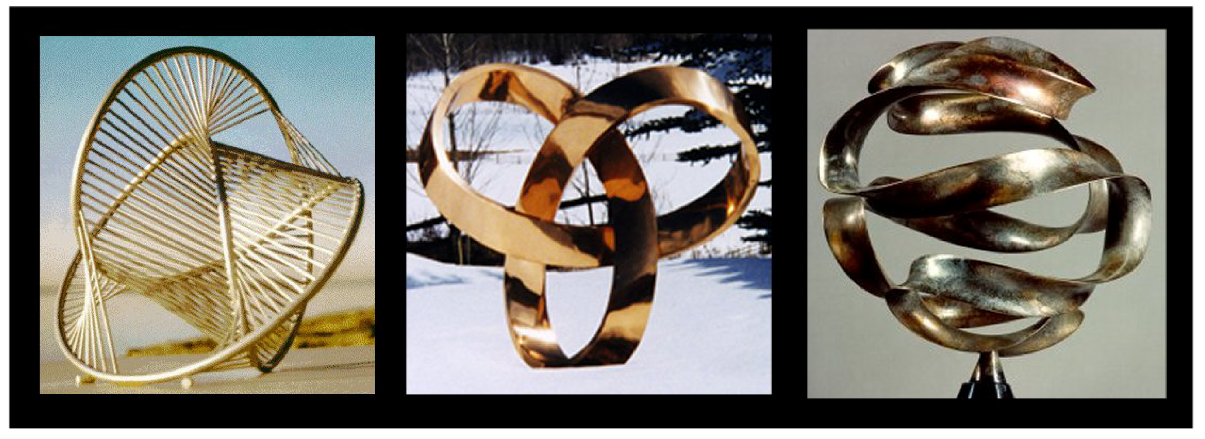
Although knots are usually viewed as one-dimensional objects in 3-dimensional space they can also be viewed on a two-dimensional surface. In particular, to every knot we can assign a special kind of surface whose boundary is the knot itself, called the Seifert surface. Knots, links, self-avoiding curves derived from them, and Seifert surfaces are very successfully used in sculpture beginning from 1930s, e.g., in the works by Naum Gabo, John Robinson, Charles O. Perry, Carlo Sequin, and Brent Collins (Figure 33). In the contemporary art typical examples are sculptures by Bathsheba Grossman [30] created by the program Seifert View by J.J. van Wijk [31], or sculptures by A. Bulatov [32].
Indonesian weaving and Tamari balls inspired the original tensegrity researchers B. Fuller and K. Snelson to use knots and links in architecture. Their approach became more popular during the last decades, with the use of light-weight materials, tensegrity and computer design tools (CAD/CAM). Some recent architectural projects, like Water cube in Beijing, based on the Waire–Phela structure that offers the better solution of the Kelvin conjecture about optimal partition of the space into cells of equal volume with the least possible area of surface between them (i.e., what is the most efficient soap bubble foam), or UNStudio Möbius house and Mercedes-Benz Museum, Stuttgart, inspired by a Möbius strip and interpretation of a trefoil knot as a boundary of its Seifert surface opened up the possibility to think about the other worlds, different from Cartesian grids, polyhedra, or uniformly spaced grid systems that dominated architecture for centuries [33]. These projects were initiated using ideas from topology, minimal surfaces, knots, links, or non-uniform space tessellations.
From mathematical point of views, diagrams representing knots or links are planar 4-valent graphs embedded in a sphere or plane with extra information determining the over-under relation of the strands. In architecture, such diagrams on a sphere can be easily transformed, by choosing a basic face, to the semi-spherical constructions of the form suitable for the construction of flexible roofs or cupolas. Embedding 4-valent graphs on non-planar surfaces different than spheres is an interesting mathematical problem with a huge potential for applications in architecture.
5.1. Polyhedral Knots and Links
Because of their regularity and symmetry, polyhedra attracted the attention of mathematicians, natural scientists, and architects for centuries. We propose several constructions of knots and links originating from regular, uniform (Archimedean), and other polyhedra. Knots and links obtained in this way preserve important symmetry properties of the original polyhedron and represent the basis for the construction of polyhedral knotted structures from nano- to the macro-level.
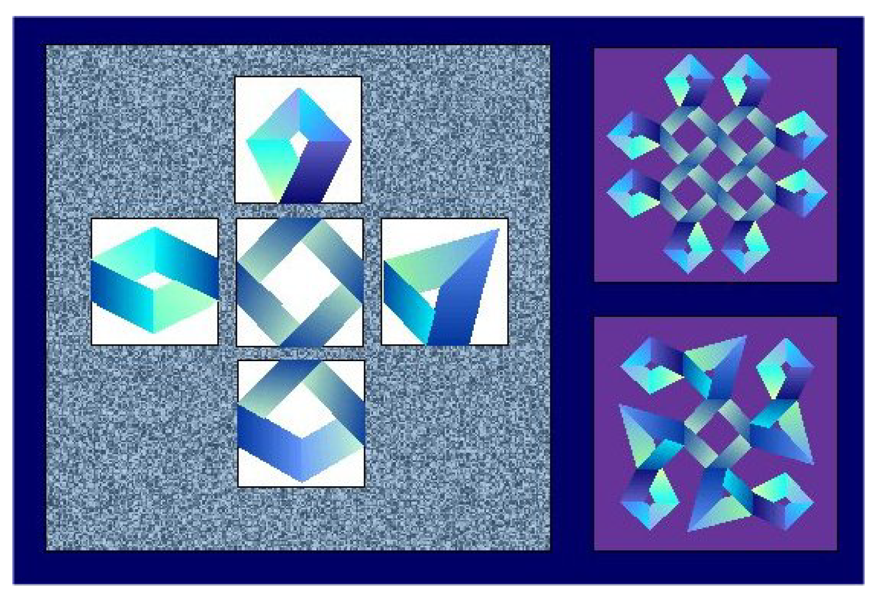
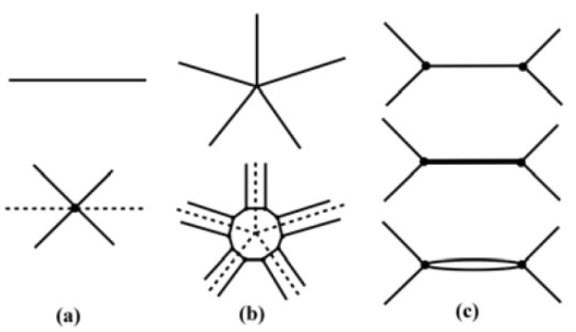
The term “polyhedral links” stands for knots and links derived from different geometric polyhedra by the mid-edge construction (Figure 34a) or cross-curve and double-line covering (Figure 34b), as well as the alternating source links derived from 3-valent geometric polyhedra by edge doubling (Figure 34c).
The middle graph of a polyhedral graph G, is obtained by connecting the mid-edge points of G (Figure 35a) belonging to the adjacent edges of G. The resulting is always a 4-valent graph, i.e., a basic polyhedron. On the other hand, every at least 3-vertex connected basic polyhedron is the middle graph of some geometrical polyhedron. Let be a link diagram obtained from by turning 4-valent vertices into over-crossings and under-crossings in an alternating manner. Notice that the initial graph G is the underlying graph of the link diagram , i.e., . Hence the middle graph construction and turning a diagram into a graph by forgetting the over-under information are in some sense mutually inverse or dual. If the original graph G does not contain digons as the faces, the same holds for its middle graph.
A new approach to the understanding the construction of polyhedral links has been developed in the papers [35,36]. These new methods involve the “cross-curve and double-line covering” construction based on the Platonic and Archimedean solids (Figure 36). The cross-curve and edge doubling construction are needed in order to obtain 4-valent graphs. The cross-curve construction consist of replacing n-valent vertices of a polyhedral graph by n-cross-curves, and then joining the adjacent loose ends to obtain a double-line covering.
Edge doubling construction (Figure 37b) can be used for obtaining 4-regular graphs from 3-regular graphs: One of the three edges of a 3-regular graph is replaced by a double edge (digon) [37]. In particular, the edge doubling construction can be applied to graphs of truncated polyhedra of fullerene graphs, which are always 3-valent, yielding various polyhedral source links.
With the advance of digital techniques and availability of ultra-light materials, ground plans representing shadows of knots and links now become 3D structures made from flexible elastic rods (Figure 38). Instead of rigid bodies, buildings of the future can be transformable entities arising from flat 4-valent nets to their embeddings, similar to the NODUS-structures proposed by D. Kozlov [38]. Frequently used geodesic domes based mostly on rigid 3-valent graphs can be replaced by 4-valent flexible geodesic domes or complex knots and links resembling the structure of natural sponges [39].
6. Conclusions
The discovery of knots probably predates that of fire or wheel. Ropes, cords and the knots that are needed to secure them played an important role in the early technological development. The main reason for the lack of discovery of such artifacts is that they have been made from organic materials (vegetable fibres, sinews, thongs, hair, etc.) and are thus subject to decay. The indirect testimony for an early use of cordage and knots are perforated objects, beads or pendants, dating some 300,000 years ago, and spherical stones found in Africa and China (about 500,000 years old), probably used as bola weights in hunting. More recently bows and arrows that required well-made cordage and secure knots, as well as Paleolithic figurine in soft limestone from Kostenki (Russia, 24, 000 B.C.) show belts made from multiple twined flexible elements. Few knots from Neolith are preserved in North Zealand and Denmark. Sophisticated plaits made with strips of date palm leaf originate from Ancient Egypt. Arrangements of knots served as a basis for mathematical recording systems in the Peruvian quipus or Zuñi knots in New Mexico, where knots were used as symbolic and mnemonic devices. Various examples of knot-art can be found in all ancient civilizations, in Japanese and Chinese art, Celtic art, ethnic Tamil and Tchokwe art, in Arabian, Greek or Smyrnian laces… The extensive use of knot-work pictures created for decorative and religious purposes in Celtic art required a high level of mathematics. Fine examples include knotted curves even with zoomorphic ornaments. Sophisticated knot constructions can be found in the works of two most prominent Renaissance artists and mathematicians: Leonardo and Dürer, as well as in Michelangelo’s drawings. In modern art, this approach is represented in creations of Naum Gabo and other constructivist sculptors.
We have barely touched numerous applications of knots in art, and discussed only few in detail, for example those based on mirror-curves or polyhedral structures. Some other examples of knot art, like Persian mosaics (and knots in mosaics in general), lace, textile, macrame, etc., remain out of the scope of this paper, together with knots in computer art. One of the most remarkable examples where mathematics (knot theory), computer science and art meet is computer software KnotPlot [40] by Rob Scharein—it will be a subject of our future paper focusing on the role of knots in art and science.
Acknowledgments
The authors express their gratitude to the Ministry of Science and Technological Development of Serbia for providing partial support for this project (Grant No. 174012).
References
- Przytycki, J.H. Knots: From combinatorics of knot diagrams to combinatorial topology based on knots. Available online: http://arxiv.org/pdf/math/0703096.pdf (accessed on 31 May 2012).
- Bain, G. Celtic Art—The Methods of Construction; Dower: New York, NY, USA, 1973. [Google Scholar]
- Allen, J.R. Celtic Art in Pagan and Cristian Times; Methuen and Co.: London, UK, 1904. [Google Scholar]
- Gerdes, P. Sona Geometry from Angola: Mathematics of an African Tradition; Polimetrica International Science Publishers: Monza, Italy, 2006. [Google Scholar]
- Gerdes, P. Geometry from Africa: Mathematical and Educational Explorations; The Mathematical Association of America: Washington, DC, USA, 1999. [Google Scholar]
- Lissajous Knot. Available online: http://en.wikipedia.org/wiki/Lissajous_knot (accessed on 31 May 2012).
- Conway, J. An Enumeration of Knots and Links and Some of Their Related Properties. In Proceedings of the Conference Computational Problems, AbstractAlgebra, Oxford 1967; Leech, J., Ed.; Pergamon Press: New York, NY, USA, 1970. [Google Scholar]
- Gerdes, P. Reconstruction and extension of lost symmetries. Comput. Math. Appl. 1989, 17, 791–813, (Also In Symmetry: Unifying Human Understanding II; Hargittai, I., Ed.; Pergamon Press: Oxford, UK, 1986). [Google Scholar] [CrossRef]
- Gerdes, P. On ethnomathematical research and symmetry. Symmetry Cult. Sci. 1990, 1, 154–170. [Google Scholar]
- Gerdes, P. Une tradition géométrique en Afrique—Les dessins sur le sable, Volume 3: Analyse Comparative; L’Harmattan: Paris, France, 1995. [Google Scholar]
- Gerdes, P. Ethnomathematik dargestellt am Beispiel der Sona Geometrie; Spektrum Verlag: Heidelberg, Germany, 1997. [Google Scholar]
- Gerdes, P. Adventures in the World of Matrices; Nova Science Publishers (Series Contemporary Mathematical Studies): New York, NY, USA, 2008. [Google Scholar]
- Gerdes, P. Lunda Geometry: Mirror Curves, Designs, Knots, Polyominoes, Patterns, Symmetries; Lulu: Morrisville, NC, USA, 2007. [Google Scholar]
- Jablan, S.V. Mirror generated curves. Symmetry Cult. Sci. 1995, 6, 275–278. [Google Scholar]
- Grünbaum, B.; Shephard, G.C. Tilings and Patterns; W.H.Freeman: New York, NY, USA, 1986. [Google Scholar]
- Cromwell, P.R. Celtic knotwork: Mathematical art. Math. Intell. 1993, 15, 36–47. [Google Scholar] [CrossRef]
- Martin, G.E. Transformation Geometry; Springer-Verlag: New York, NY, USA, 1980. [Google Scholar]
- Jablan, S.V. Symmetry, Ornament and Modularity, Series on Knots and Everything 30; World Scientific: Singapore, 2002. [Google Scholar]
- Shubnikov, A.V.; Koptsik, V.A. Symmetry in Science and Art; Plenum Press: New York, NY, USA, 1974. [Google Scholar]
- Coxeter, H.S.M.; Moser, W.O.J. Generators and Relations for Discrete Groups; Springer-Verlag: New York, NY, USA, 1980. [Google Scholar]
- Washburn, D.; Crowe, D.W. Symmetries of Culture; University of Washington Press: Seattle, DC, USA, 1988. [Google Scholar]
- Emery, I. The Primary Structures of Fabrics. In Watson-Guptill Publications/Whitney Library of Design; The Textile Museum: Washington, DC, USA, 1995. [Google Scholar]
- Crowe, D.W. Introduction to Slavik Jablan’s Modular Games. Available online: http://www.emis.de/journals/NNJ/Crowe.html (accessed on 31 May 2012).
- Fathauer, R. KnoTiles. Available online: http://mathartfun.com/shopsite_sc/store/html/Tessellations/MakingFaces.html (accessed on 31 May 2012).
- Lomonaco, S.J.; Kauffman, L.H. Quantum knots and mosaics. Quantum Inf. Process. 2008, 7, 85–115. [Google Scholar] [CrossRef]
- Kuriya, T. On a lomonaco-kauffman conjecture. 2008. Available online: http://arxiv.org/pdf/1106.3784.pdf (accessed on 31 May 2012).
- Sossinsky, A. Knots—Mathematics with a Twist; Harvard University Press: Cambridge, MA, USA, 2002. [Google Scholar]
- Jablan, S.; Radović, L.J.; Sazdanović, R.; Zeković, A. Mirror-curves and knot mosaisc. Comput. Math. Appl. 2011, arXiv:1106.3784v2 [math.GT]. [Google Scholar]
- Tkalec, U.; Ravnik, M.; Čopar, S.; Žumer, S.; Muševič, I. Reconfigurable knots and links in chiral nematic colloids. Science 2011, 333, 62–65. [Google Scholar] [CrossRef] [PubMed]
- Grossman, B. Bathsheba Sculpture. Available online: http://www.bathsheba.com/ (accessed on 31 May 2012).
- Van Wijk, J.J. Seifert View. Available online: http://www.win.tue.nl/~vanwijk/seifertview/ (accessed on 31 May 2012).
- Bulatov, A. Bulatov Abstract Creations. Available online: http://bulatov.org/ (accessed on 31 May 2012).
- Vallisser, T. Other Geometries in Architecture: Bubbles, Knots and Minimal Surfaces. Available online: http://www.springer.com/cda/content/document/cda_downloaddocument/978-88-470-1121-2_Wallisser.pdf (accessed on 31 May 2012).
- Mathematica Polyhedron Data. Available online: http://reference.wolfram.com/mathematica/ref/PolyhedronData.html/ (accessed on 31 May 2012).
- Zhang, Y.; Seeman, N.C. Construction of a DNA-truncated octahedron. J. Am. Chem. Soc. 1994, 116, 1661–1669. [Google Scholar] [CrossRef]
- Qiu, W.-Y.; Zhai, X.-D. Molecular design of Goldberg polyhedral links. J. Mol. Struc. (Theochem) 2005, 756, 163–166. [Google Scholar] [CrossRef]
- Jablan, S.; Sazdanović. LinKnot—Knot Theory by Computer; World Scientific: New Jersey, NJ, USA; London, UK; Singapore, 2007; Available online: http://math.ict.edu.rs/ or http://www.mi.sanu.ac.rs/vismath/linknot/index.html; (accessed on 31 May 2012). [Google Scholar]
- Kozlov, D. Topological Method of Construction of Point Surfaces as Physical Models. Available online: http://www.marhi.ru/AMIT/2008/spec08/papers/Kozlov/Kozlov02_paper_EAEA2007.pdf (accessed on 31 May 2012).
- Burt, M. Periodical Sponge Structures and Uniform Sponge Polyhedra in Nature and in the Realm of the Theoretically Imaginable. Vismath 2007, 9, 4. Available online: http://www.mi.sanu.ac.rs/vismath/burt/index.html (accessed on 31 May 2012).
- Scharein, R. KnotPlot. Available online: http://knotplot.com/ (accessed on 31 May 2012).
Figure 1.
(a) Cylinder seal, Ur, Mesopotamia, ca. 2600–2500 B.C.; (b) stamp seals, Anatolia, ca. 1700 B.C.
Figure 1.
(a) Cylinder seal, Ur, Mesopotamia, ca. 2600–2500 B.C.; (b) stamp seals, Anatolia, ca. 1700 B.C.

Figure 2.
Chinese traditional decorative knots.

Figure 3.
Closure of the crossed noose that gives the knot .

Figure 4.
Hercules knot, Greek jewelry, Pontika (Ukraina), 300 B.C.

Figure 5.
Greek mosaic that can be transformed into the link .

Figure 6.
Celtic knot designs.

Figure 7.
s obtained from for .

Figure 8.
s obtained from for .

Figure 9.
Tamil designs.

Figure 10.
Tchokwe sand drawings.

Figure 11.
Leonardo’s Concatenation.

Figure 12.
Knot design obtained from a uniform tiling.

Figure 13.
A mirror placed in a crossing point of (a) two different curves; (b) one curve.

Figure 14.
The successive introduction of internal mirrors in the that preserves a single curve.

Figure 15.
Construction of a single mirror curve from the tiling (a) by connecting edge mid-points (b); tracing components (c) and introducing a mirror (d).
Figure 15.
Construction of a single mirror curve from the tiling (a) by connecting edge mid-points (b); tracing components (c) and introducing a mirror (d).

Figure 16.
Rules for composing plate designs and mirror curves.

Figure 17.
Algorithm for creating monolinear symmetric mirror curves.

Figure 18.
Celtic tangles.

Figure 19.
Celtic knots, friezes and plane knotwork ornaments.

Figure 20.
Celtic circle and square knot designs.

Figure 21.
(a) ‖-direct product in the Tchokwe design; (b,c) the application of Rule 3 in Tchokwe designs.
Figure 21.
(a) ‖-direct product in the Tchokwe design; (b,c) the application of Rule 3 in Tchokwe designs.

Figure 22.
Derivation of Celtic monolinear cross knot design from plate design obtained using the Rule 4.
Figure 22.
Derivation of Celtic monolinear cross knot design from plate design obtained using the Rule 4.

Figure 23.
Celtic monolinear knot cross design.

Figure 24.
Celtic mirror curves.

Figure 25.
Celtic monolinear design with broken symmetry.

Figure 26.
Construction of Celtic monolinear knot design (b) by breaking the symmetry of the two-component symmetric design (a).
Figure 26.
Construction of Celtic monolinear knot design (b) by breaking the symmetry of the two-component symmetric design (a).

Figure 27.
Celtic friezes with the same symmetry group of bands p1a1.

Figure 28.
Celtic friezes with the same symmetry group of bands p121.

Figure 29.
KnotTiles by S. Jablan.

Figure 30.
Figure-eight knot and Borromean rings as knot mosaics [25].
Figure 30.
Figure-eight knot and Borromean rings as knot mosaics [25].


Figure 32.
Borromean rings synthesized in chiral nematic colloids [29] and missing links and .
Figure 32.
Borromean rings synthesized in chiral nematic colloids [29] and missing links and .

Figure 33.
Sculptures by Charles O. Perry, John Robinson, and Brent Collins.

Figure 34.
(a) Mid-edge construction; (b) cross-curve and double-line covering construction; (c) edge doubling construction. Broken lines denote edges of the original graph deleted during the construction.
Figure 34.
(a) Mid-edge construction; (b) cross-curve and double-line covering construction; (c) edge doubling construction. Broken lines denote edges of the original graph deleted during the construction.

Figure 35.
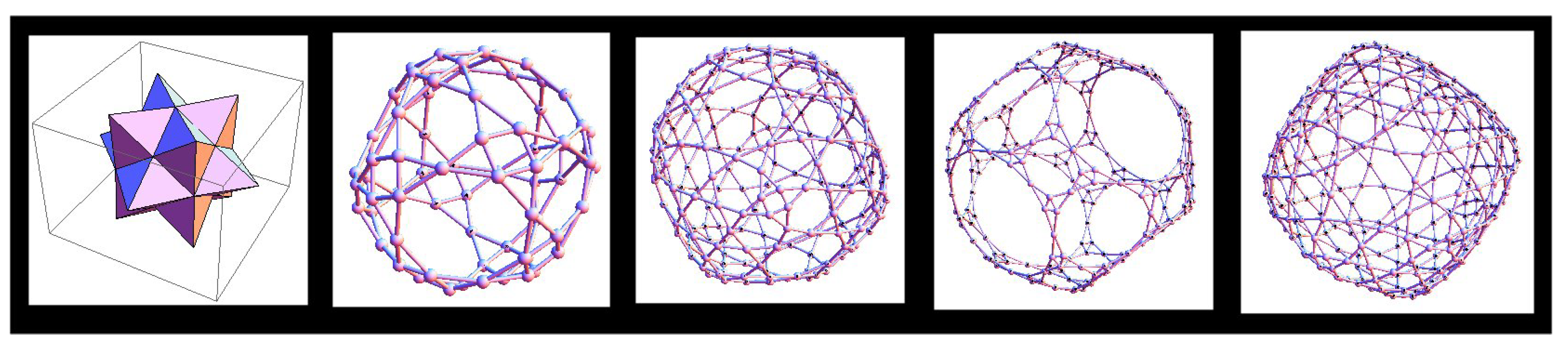
Escher’s solid from the Mathematica data base of polyhedra [34] and basic polyhedra obtained from it and its transforms (truncated, stellated and geodesated Escher solid) by mid-edge construction.
Figure 35.
Escher’s solid from the Mathematica data base of polyhedra [34] and basic polyhedra obtained from it and its transforms (truncated, stellated and geodesated Escher solid) by mid-edge construction.

Figure 36.
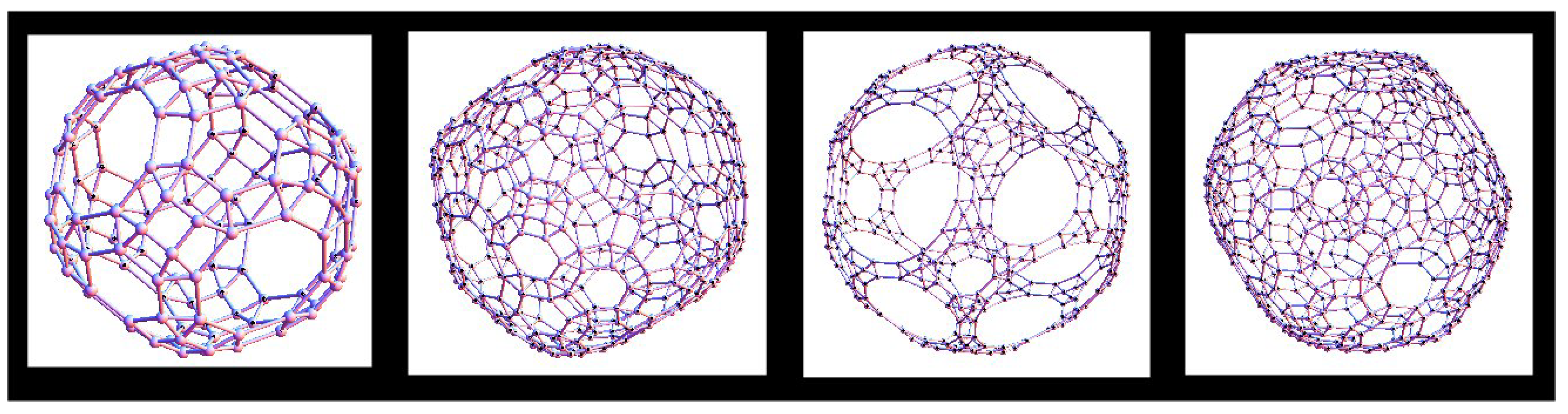
Basic polyhedra obtained from Escher’s solid and its transforms by cross-curve and double-line covering.
Figure 36.
Basic polyhedra obtained from Escher’s solid and its transforms by cross-curve and double-line covering.

Figure 37.
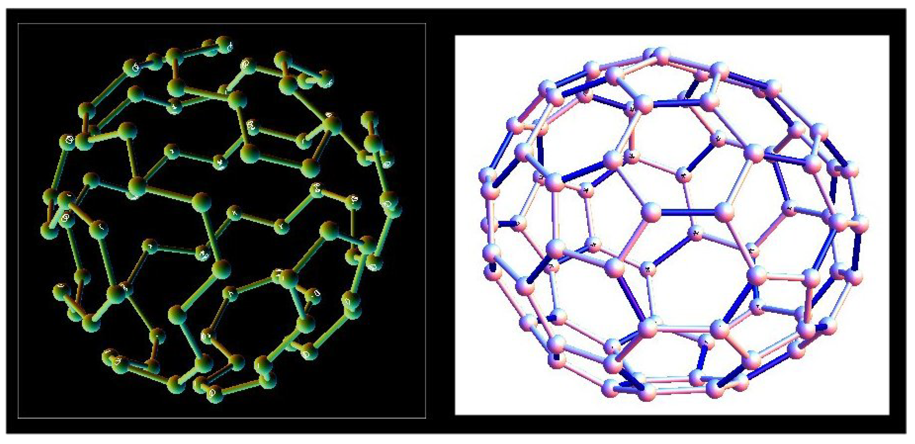
Hamiltonian cycle on fullerene and edge doubling applied to .

Figure 38.
A Seifert surface corresponding to knot and different polyhedral knots and links.

© 2012 by the authors; licensee MDPI, Basel, Switzerland. This article is an open access article distributed under the terms and conditions of the Creative Commons Attribution license (http://creativecommons.org/licenses/by/3.0/).
Share and Cite
MDPI and ACS Style
Jablan, S.; Radović, L.; Sazdanović, R.; Zeković, A. Knots in Art. Symmetry 2012, 4, 302-328. https://doi.org/10.3390/sym4020302
AMA Style
Jablan S, Radović L, Sazdanović R, Zeković A. Knots in Art. Symmetry. 2012; 4(2):302-328. https://doi.org/10.3390/sym4020302
Chicago/Turabian StyleJablan, Slavik, Ljiljana Radović, Radmila Sazdanović, and Ana Zeković. 2012. "Knots in Art" Symmetry 4, no. 2: 302-328. https://doi.org/10.3390/sym4020302