Diagrammatics in Art and Mathematics

Abstract

This paper explores two-way relations between visualizations in mathematics and mathematical art, as well as art in general. A collection of vignettes illustrates connection points, including visualizing higher dimensions, tessellations, knots and links, plotting zeros of polynomials, and new and rapidly developing mathematical discipline, diagrammatic categorification.

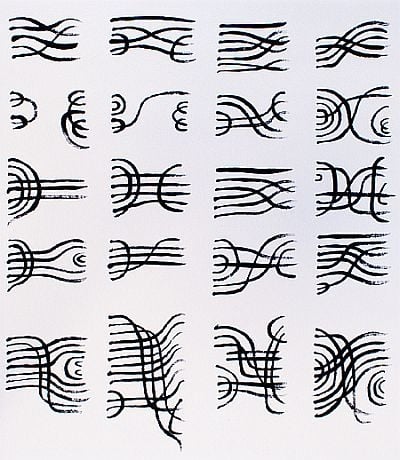
1. Introduction

The relation between mathematics and art is long lasting and constantly evolving, but it is usually seen as one way: from mathematical objects to their visualizations. Numerous examples include fractals, tessellations, knots and links, dynamical systems, and Platonic solids. On the other hand, visualizations naturally lend themselves to mathematics and can be used to simplify long computations, develop the intuition, and aid the proofs. Rob Kirby developed a diagrammatic calculus together with the finite set of moves for visualizing 3-manifolds and smooth 4-manifolds by surgery on framed links [1].

A snapshot from the movie Visualizing Seven-Manifolds [2] by N. Johnson (Figure 1) illustrates J. Milnor’s construction of two smooth seven-dimensional manifolds which are homeomorphic to the standard seven-sphere. The one on the left, $S_1^7$ is diffeomorphic to the standard seven-sphere, but the one on the right, $S_3^7$, is not—such a manifold is said to be exotic. Both manifolds are obtained by gluing two copies of $S^3\times D^4$ along their boundary via a map ${\xi }_{h,j}:S^3\to SO\left(3\right)$. The 3-sphere is drawn, via stereographic projection, as a 3-dimensional ball. The large circles are fibers of the Hopf fibration; at each point along these circles we see instructions for gluing two 4-dimensional balls into a 4-sphere. These instructions are indicated by two reference circles in the standard 4-ball: at center we see the standard position of these two circles (blue and red). The gluing map ${\xi }_{h,j}$ deforms them to the corresponding circles shown along the Hopf fibers. One such deformation is drawn larger in front of the others, and here we also draw the image of the equatorial two-sphere in $S^3$. The difference in configurations of these red and blue circles indicates the difference in diffeomorphism types of the corresponding seven-spheres.

A new and rapidly developing area of mathematics, called categorification, relies on various kinds of diagrams in low-dimensions: two, three and four. Recent examples include categorification of various polynomial invariants for knots and links, such as Khovanov link homology [3] and Knot Floer homology, independently developed by Ozsvath–Szabo and Rasmussen, which lift the Jones and the Alexander polynomial, as well as categorification of quantum groups.

2. Modeling the Universe: Tessellations

The universe is an inexhaustible source of questions for scientists and mathematicians. The puzzle of spiral galaxies was an excellent problem in 1963, according to R. Feynman, more than a hundred years after Lord Rosse posed the following in 1850:

“Much as the discovery of these strange forms may be calculated to excite our curiosity, and to awaken an intense desire to learn something of the laws which give order to these wonderful systems, as yet, I think, we have no fair ground even for plausible conjecture.”

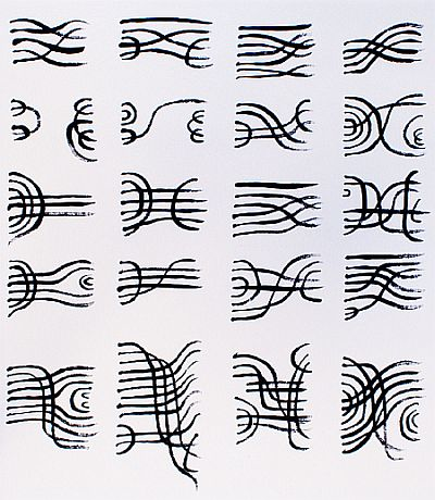
Recent work of H. Bray about density waves in dark matter and their relation to the observed spiral density waves in spiral galaxies leads to the beautiful models of spiral galaxies. Figure 2 contains the simulated image of the Spiral galaxy NGC3310 on the right obtained by running the Matlab function spiralgalaxy [4] (1, 75000, 1, −0.15, 2000, 1990, 100000000, 8.7 × 10⁻¹³, 7500, 5000, 45000000, 50000) described in paper [5]. Left photo on Figure 2 is obtained by NASA and The Hubble Heritage Team (STScI/AURA) in March 1997 and September 2000, telescope: Hubble Wide Field Planetary Camera 2.

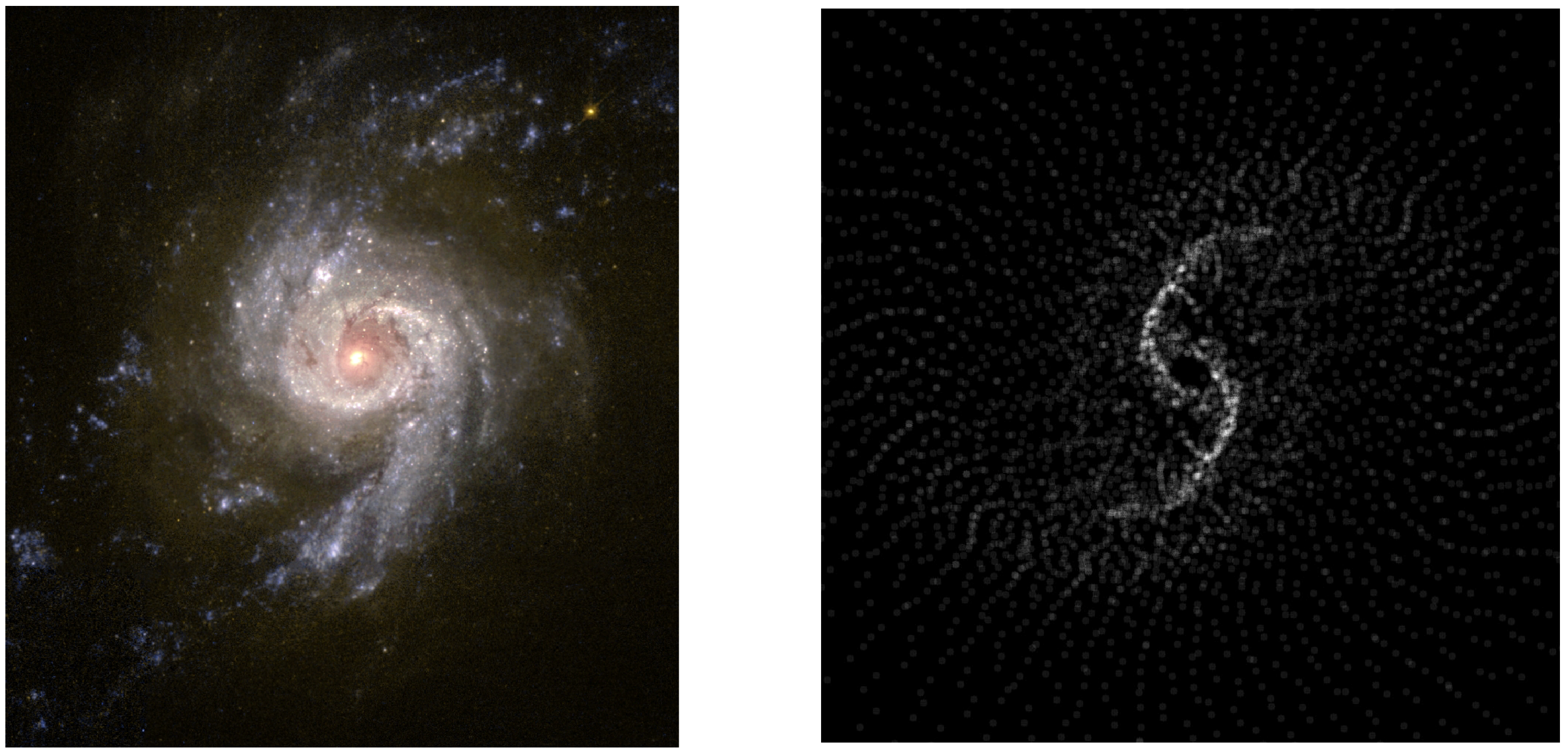
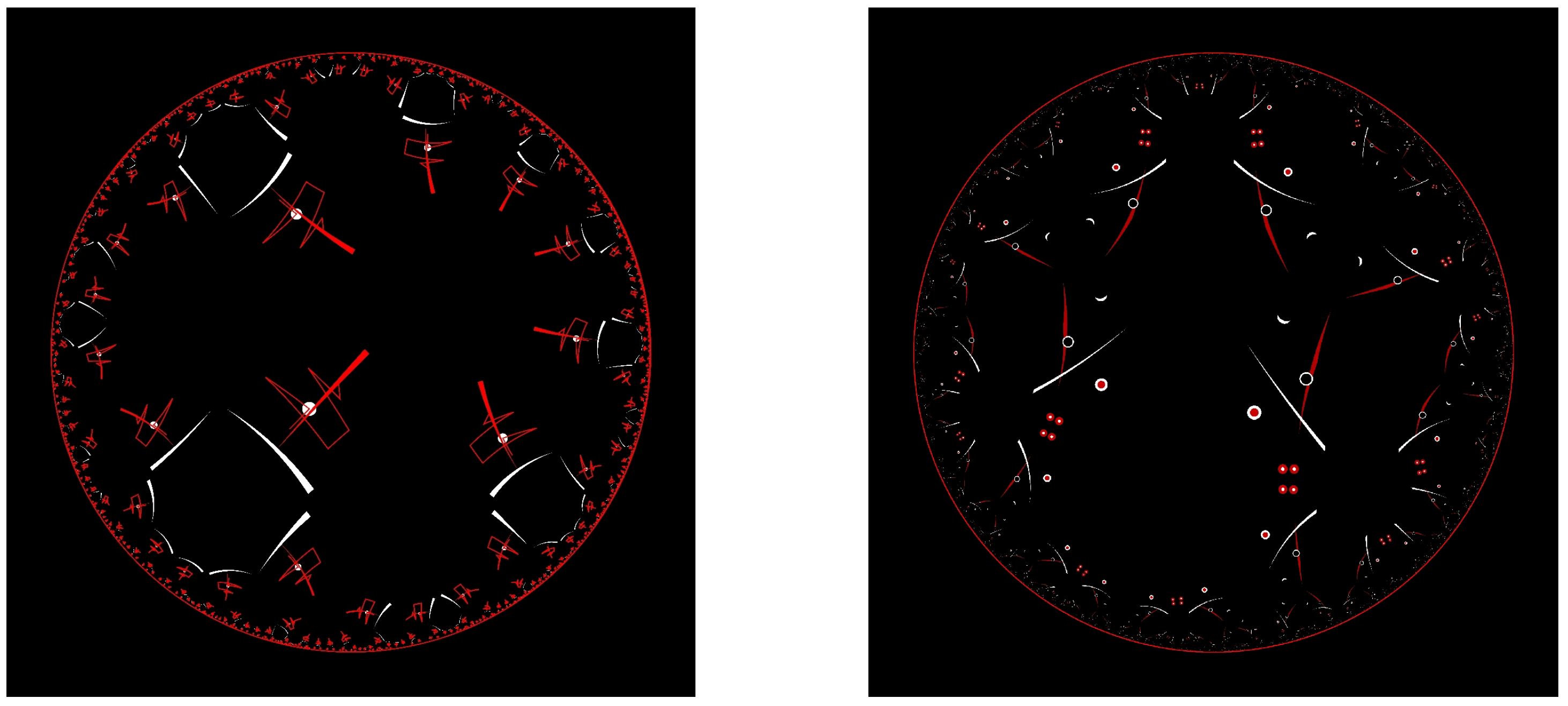
A related question about the shape of the universe is a topic of Escher’s woodcut [6], see Figure 3. Tessellations Heaven and Hell and Angels and Demons feature the same tiles, angels and demons, and depict the dichotomy between the good and bad, heaven and hell. Viewed side by side these tessellations emphasize the differences between the hyperbolic space of constant curvature minus one, and the flat Euclidean plane, flat versus curved universe.

The lack of intuition and the conviction that the V Postulate depends on first four groups of axioms was so strong that no one recognized the basis for new geometry until the early 19th century. On 8 November 1824 C.F. Gauss commented:

“The assumption that the sum of three angles is less than ${180}^{\circ }$ leads to some curious geometry, quite different than ours, but thoroughly consistent.”

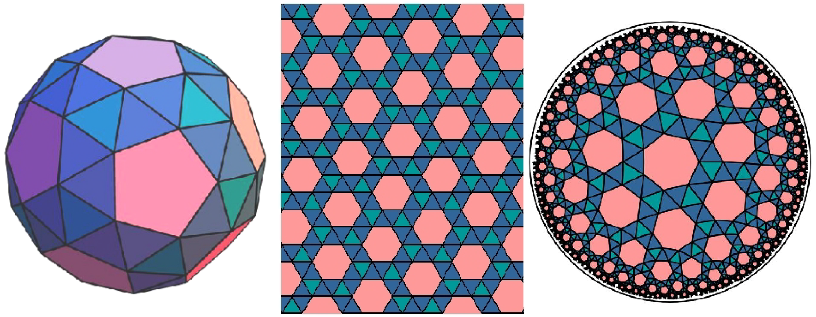
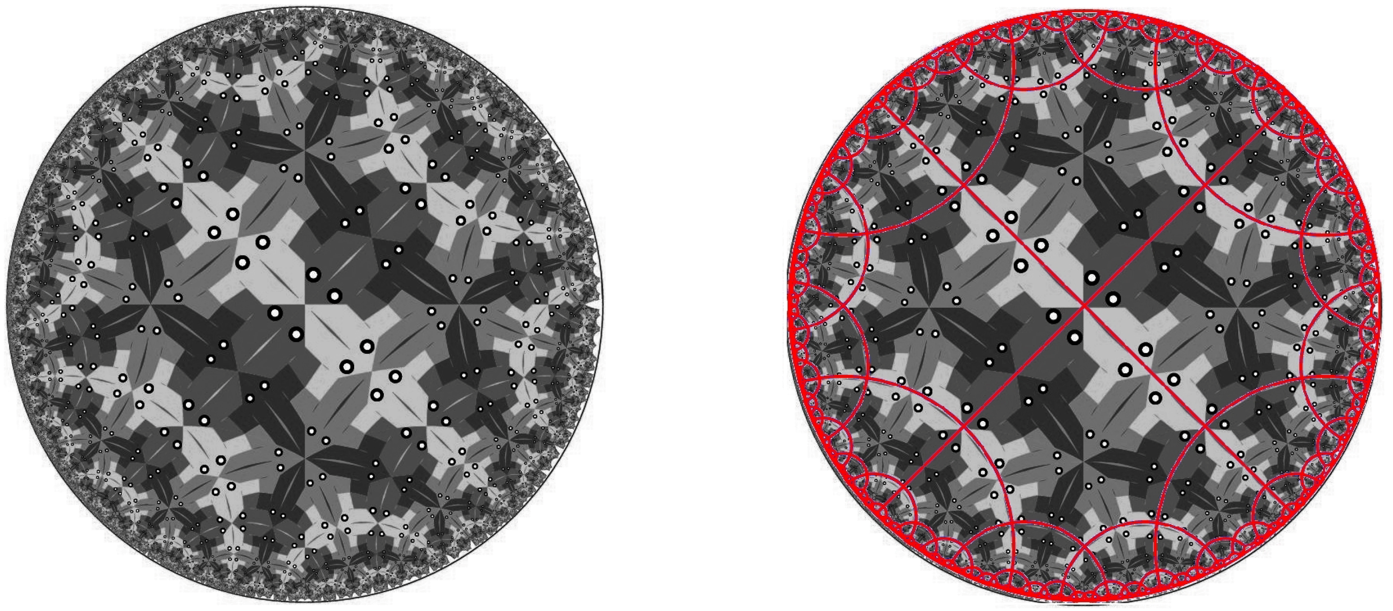
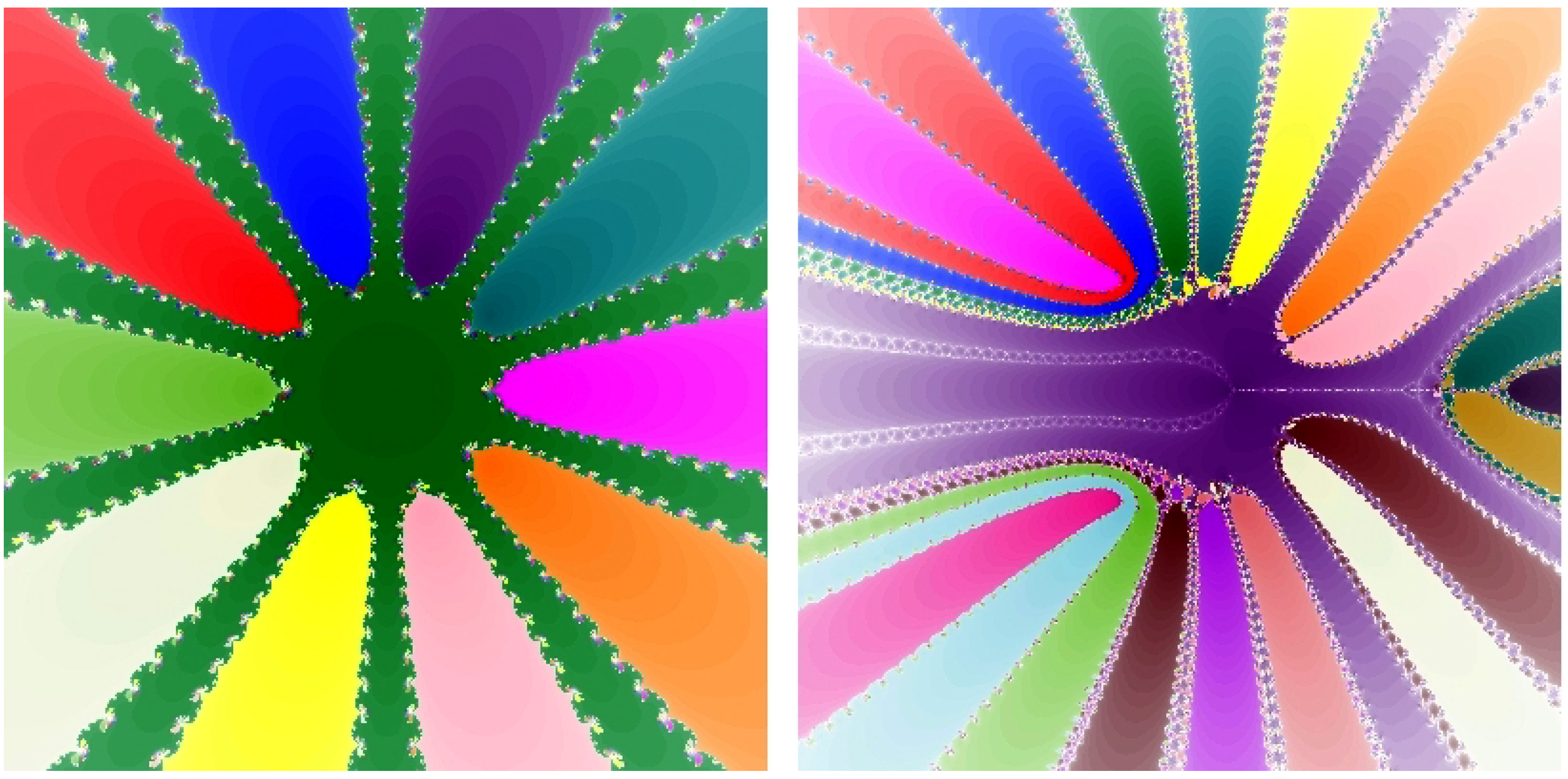
The founders of a “new geometry”, C.G. Gauss, J. Bolyai, and N. Lobachevski, were the first to deny the absolute nature of Euclidean geometry and provide us with a theory based on axiomatic methods. Visualizations of the hyperbolic plane and non-Euclidean geometry became possible with the discovery of their models within the Euclidean geometry. Three different tessellations, determined by their Schläfli symbols (Schläfli symbols determine a tessellation by specifying the polygons around each vertex of the tessellation. Notice that the correspondence between the symbol and the tessellations is one to many, i.e., the symbol does not necessarily define the tessellation uniquely.) differ only in one polygon, elliptic one has a pentagon, Euclidean a hexagon, and the hyperbolic has the heptagon, which can be informally interpreted as the amount of space available in each of the geometries, see Figure 4. The correspondence between the underlying tessellation by the regular polyhedra and the Escher-like tessellations is partially revealed on Figure 5, picture on the right shows the (red) wire model of the polygonal tessellation. (All of the tessellations in the rest of this section were created using Mathematica package Tess [7,8,9,10,11].)

There are several well-known methods for creating interesting 2-dimensional hyperbolic tessellation, such as taking the dual tessellation by connecting the incenters of the polygons in the original tessellation, superimposing, converting polygons into curvilinear domains while preserving the symmetries of the tessellation, etc. One of the most interesting methods can be described in two steps:

• Mathematics: determine the fundamental domain (region) i.e., the smallest region in the tessellation which can be used to recreate the tessellation by applying the symmetries of the tessellation.
• Art: choose a pattern to insert into the fundamental domain, and map it onto the plane via symmetries of the tessellation, along with the fundamental domain, and observe the pattern it forms.

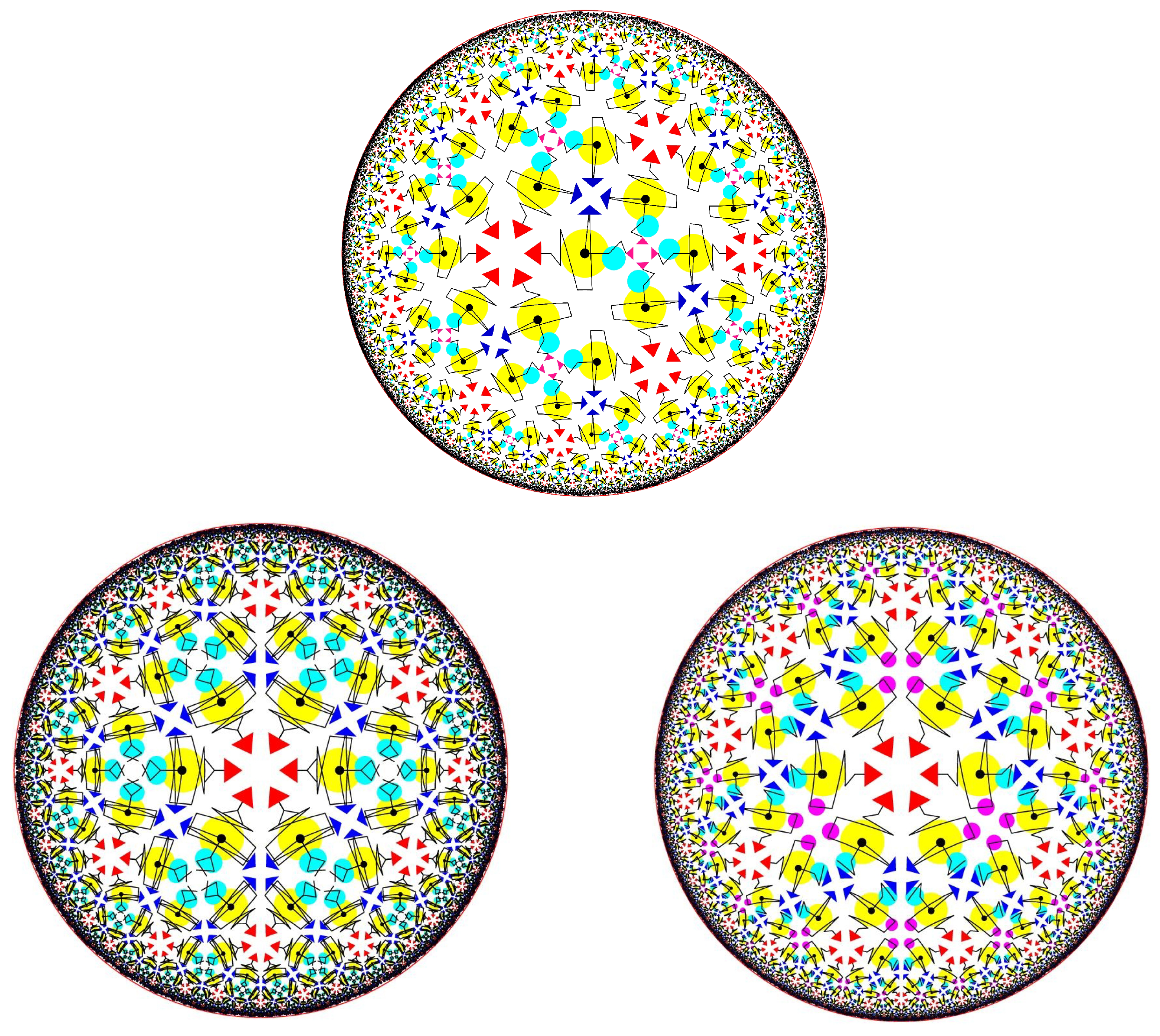
Hyperbolic twittering machine tessellation and its variations, see Figure 6, are based on the tessellation $(4,4,4,6)$. They are constructed by inserting similar patterns with a different symmetries into the fundamental domain. Patterns for two bottom tessellations differ by a reflection: the one on the left is more symmetric, notice the dark blue triangles versus the dark blue and purple triangles on the right. The Paul Klee tessellation on the top appears less symmetric because it is not centered within the unit circle. Additional complexity comes with the use of colors, but we will not discuss the colored symmetry in the paper.

Constructing the following tessellations involves disregarding the mathematical requirement of introducing the pattern within the fundamental domain. Following the genius ideas in Persian art of the medieval time and artisans creating kilims (Kilims are decorative flat tapestry-woven carpets or rugs with ornaments full of symbolism from Byzantine, Greek, Chinese and Turkish tradition.) from Balkans to Persia [12], we allow overlapping in creating the tessellations. The pattern for Poincare Berries tessellation on Figure 7 consists of thin and thick triangles, as well as circles, which cover the region a bigger than the fundamental domain. The effect of overlapping is reinforcing local four- and six-fold rotational symmetry of the $(4,4,4,6)$ tessellation. The interplay of the white weave and the pattern emphasizes the underlying structure.

Unlike Poincare Berries, tessellations in Figure 8 are inspired by Japanese tradition: pagodas for the one on the right, and Japanese warriors on the left. Both tessellations are realized in classical black, red and white color scheme on the black background, emphasizing local seven-fold and six-fold symmetry, respectively.

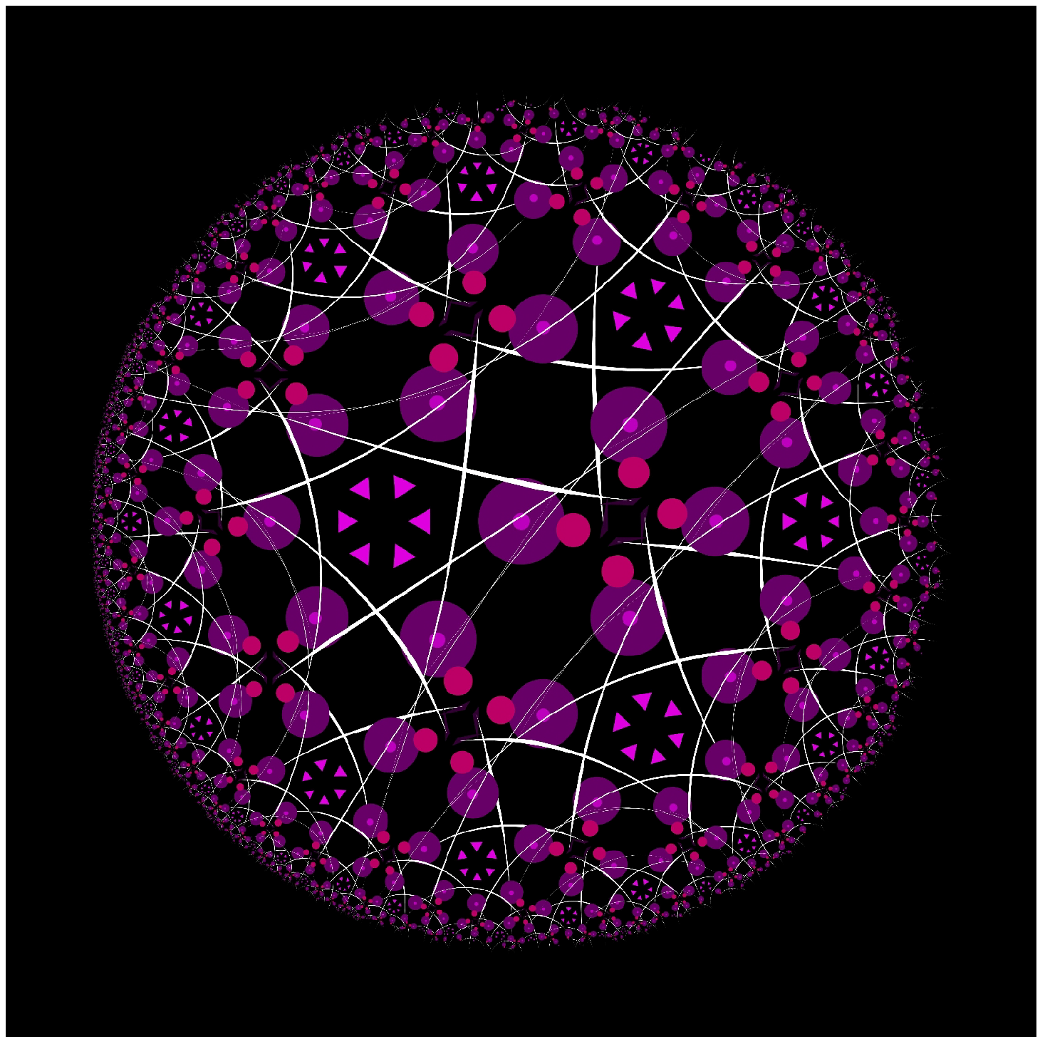
Digital print Sea Pearls, see Figure 9, by R. Sazdanovic is based on the hyperbolic tessellation $(7,7,7,7)$ and realized in the Poincare disk model. The core pattern consists of red and white circles of various sizes, and color intensities. It is extended to the whole hyperbolic plane under symmetries of the original tessellation, yet with the overall effect of breaking the symmetry of the tessellation. Note that there are infinitely many tessellations of the hyperbolic plane: all of them can be used for creating aesthetically pleasing tessellations if you are willing to experiment. It is often very hard to predict the final tessellation based on the pattern and the symmetries of the original one, especially if the pattern is larger than the fundamental domain or covers only a part of it.

3. Knot Theory: Knotting Mathematics and Art

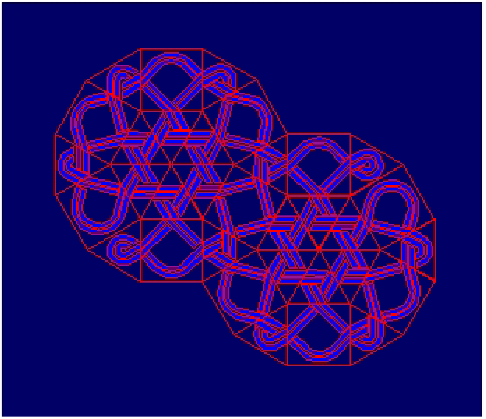
Knots play the prominent role in art history, fine examples include the Chinese and Celtic knots, Peruvian quipu, Leonardo da Vinci and Albrecht Dürer knots. Although they are intrinsically three-dimensional objects, knots can be constructed from graphs (In order to obtain all knots we need to consider signed graphs.), hence they can also be obtained from tessellations, see Figure 10.

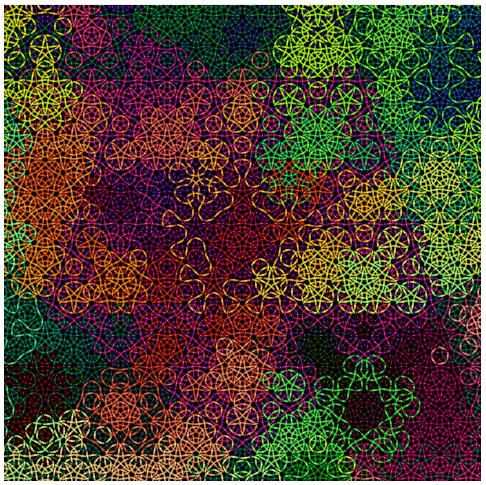
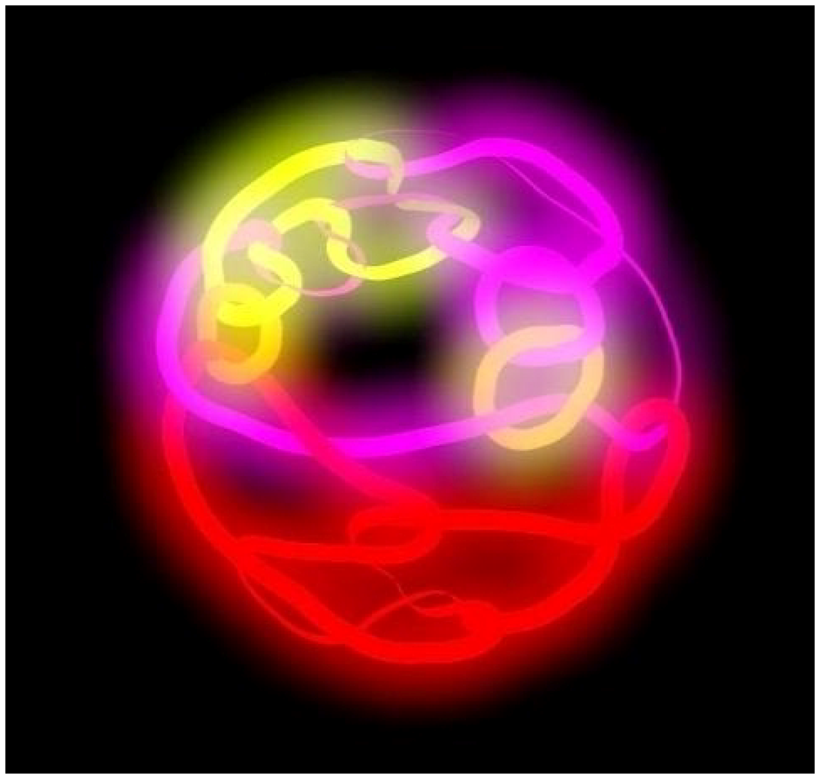
R. Scharein is the author of an infinite knot diagram whose part is shown on Figure 11. His knot is created by applying the principles of Celtic knotting to an underlying aperiodic Penrose tiling (instead of a rectangular grid). Although each individual string in the diagram has a five-fold symmetry about its geometric center, the diagram as a whole has no rotational or translational symmetries.

R. Scharein’s computer program Knotplot enables visualization and manipulating mathematical knots in three and four dimensions [13]. It was used to create Tying and untying, a short movie [14] that addresses one of the principal questions in knot theory–unknotting and distinguishing knots. More precisely, it illustrates J.H. Conway’s classification of knots and links into families. Mathematical ideas permeate vivid animations and music, creating visual-acoustic symphony, Figure 12.

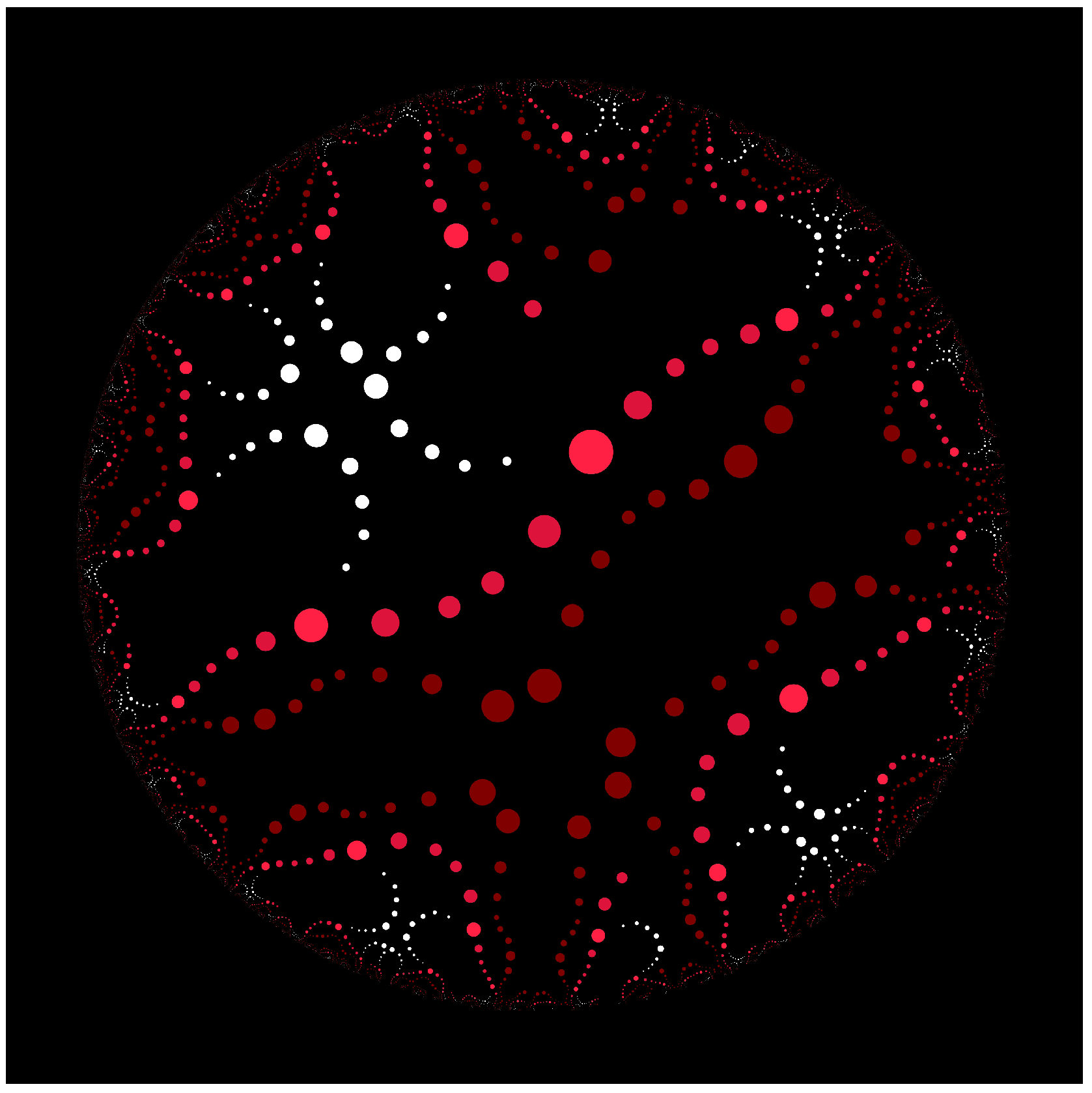
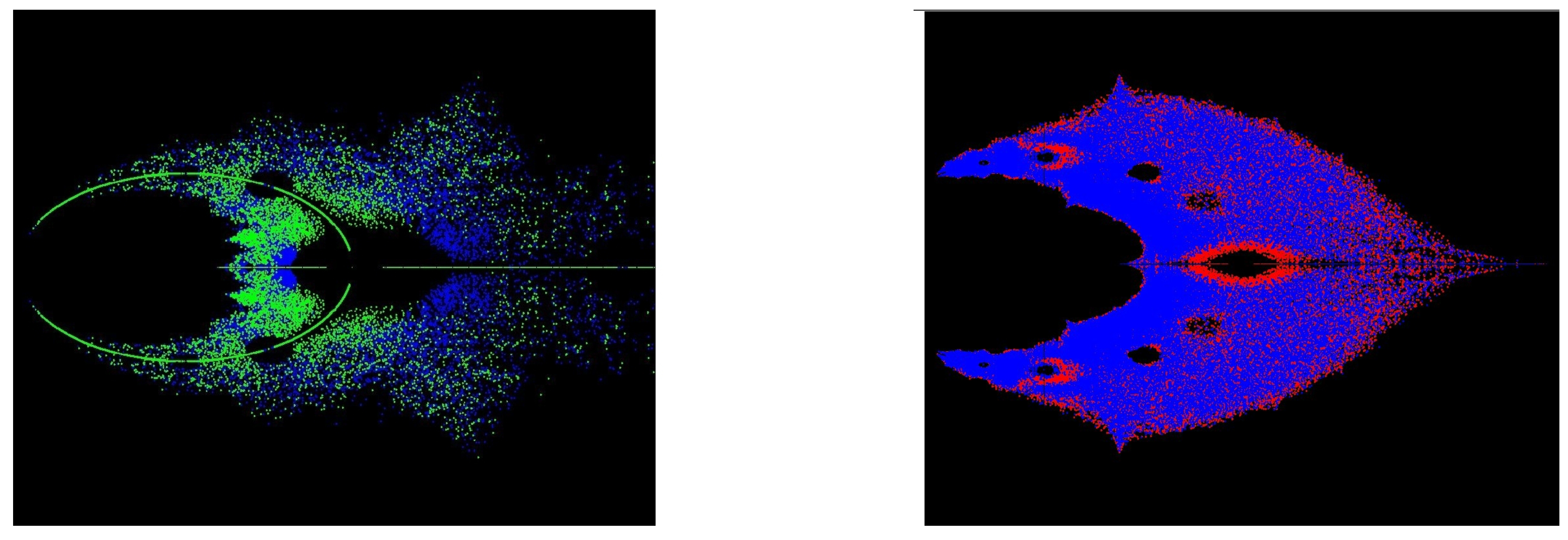
In addition to the classical approach to visualizing knots and links, see Figure 13, and their symmetries [15,16,17], S. Jablan’s work introduces a new approach to featuring knots in visual art, Figure 14 and Figure 15. Instead of visualizing knots and links directly, he is using their polynomial invariants to create his artwork. Images on Figure 14 and Figure 15, created via LinKnot [18], are plots of zeros of the certain polynomials of classes of knot and links [17]. Alexander galaxy, on the left of Figure 14, represents zeros of the Alexander polynomials of rational knots and links with at most 17 crossings, with zeros of knots plotted in green and of links in blue.

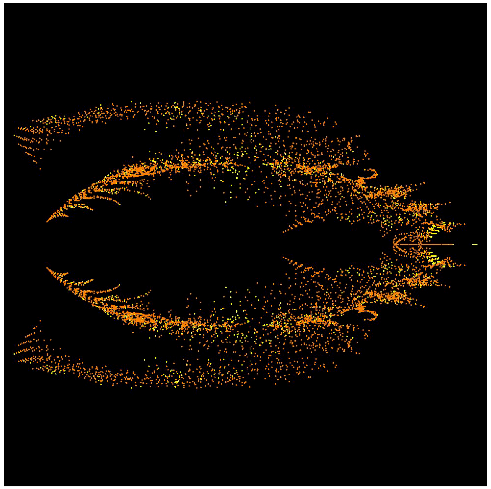
This approach can be extended to the families of graphs corresponding to knot families, and the polynomial invariants of graphs. Figure 16 contains plots of zeroes of the chromatic polynomial for the n-pyramid graph (on the left) and the Jones polynomial of the corresponding polyhedral knot $2n^{\ast }$, created using Polynomiography, computer software for visualizing approximation of zeros of polynomials by B. Kalantari [19,20].

4. Diagrammatic Categorification

In this section we will describe a few research level results for which the visualizations are essential and relevant to mathematics. A nice example where diagrammatics naturally lends itself to mathematical concepts is the bijection (the bijection is between sets) between unoriented one dimensional topological field theories over some field k and the finite dimensional k-vector spaces with a non-degenerate bilinear form. Moreover, finding the relations in a diagrammatically defined category is equivalent to finding the atomic pieces in the next higher categorical level. As an illustration of this process we offer Scott Carter’s drawing related to knotted foams, Figure 17: when the shape Y moves under an arc, in a movie, the time-elapsed form becomes a foam in which a branch line is crossed by a transverse sheet [21].

Categorification is a new area of mathematics introduced by I. Frenkel and L. Crane, and recently popularized by D. Bar-Natan and M. Khovanov [3,22]. Categorification can be thought of as a process which lifts numbers to vector spaces and vector spaces to categories. A prime example is turning Euler characteristic of a topological space into its homology groups. More exotic examples include various link homology groups which lift polynomial invariants of knots. For instance, Khovanov homology lifts the Jones polynomial, and Ozsvath–Szabo–Rassmussen homology lifts the Alexander polynomial. Motivated by categorification in knot theory and the relation of knots and planar graphs several graph invariants have also been categorified, such as the chromatic and the Tutte polynomial.

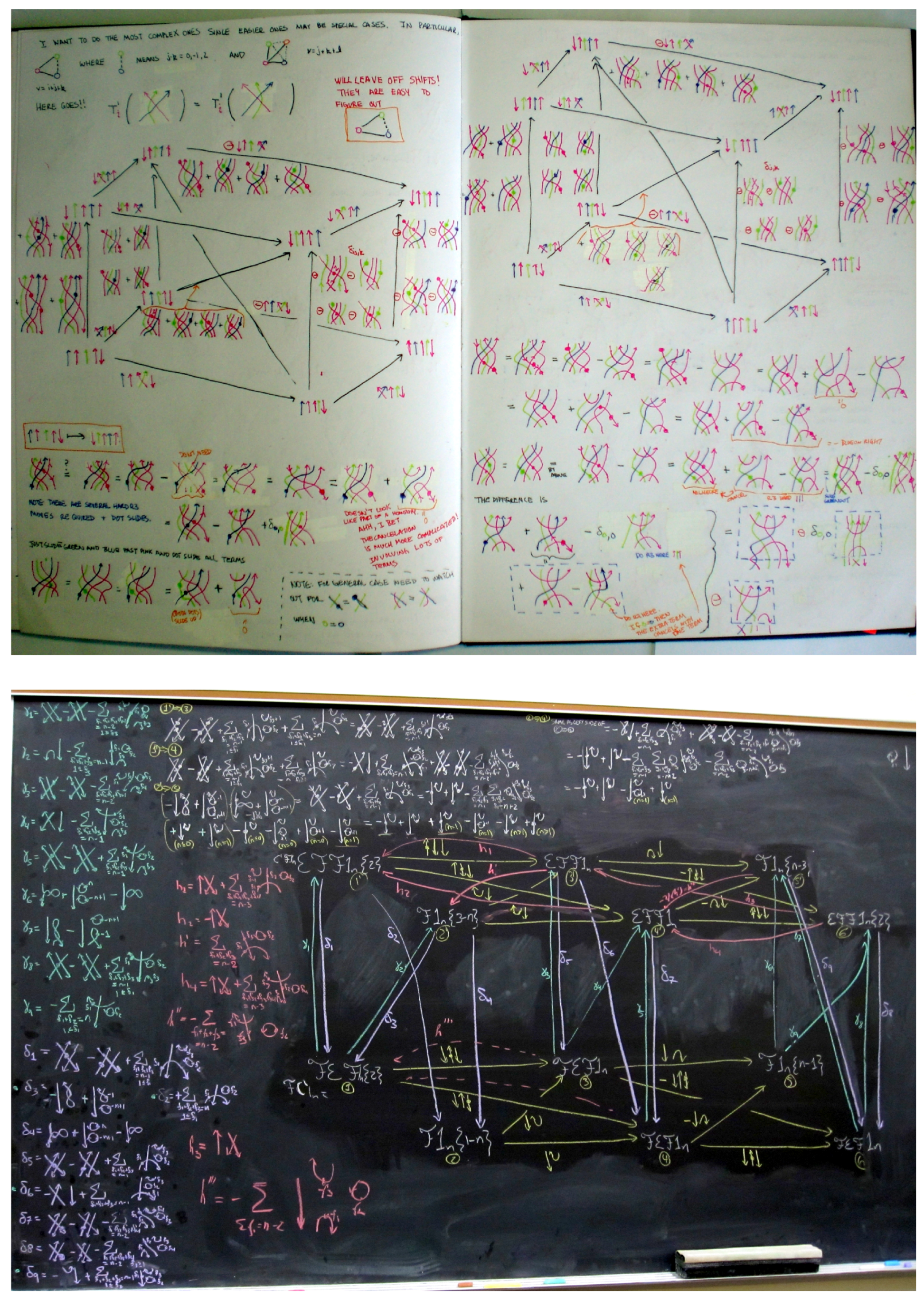
Other recent examples of diagrammatic categorification include quantum groups, Heisenberg, Hecke, Temperley–Lieb, and Schur algebras, Reshetikhin–Turaev link invariants of link, polynomial ring $Z\left[x\right]$ in the work of Cautis, Khovanov, Lauda, Licata, Sazdanovic, Stosic, Webster and many others. Figure 18 documents the creative research process: diagrams used in categorification of quantum groups and the Casimir element by A. Lauda.

Sometimes the choice of categorification diagrams is obvious:

• diagrams of knots and links for Khovanov link homology and the Knot Floer homology,
• graphs for the chromatic graph cohomology and the categorification of the Tutte polynomial.

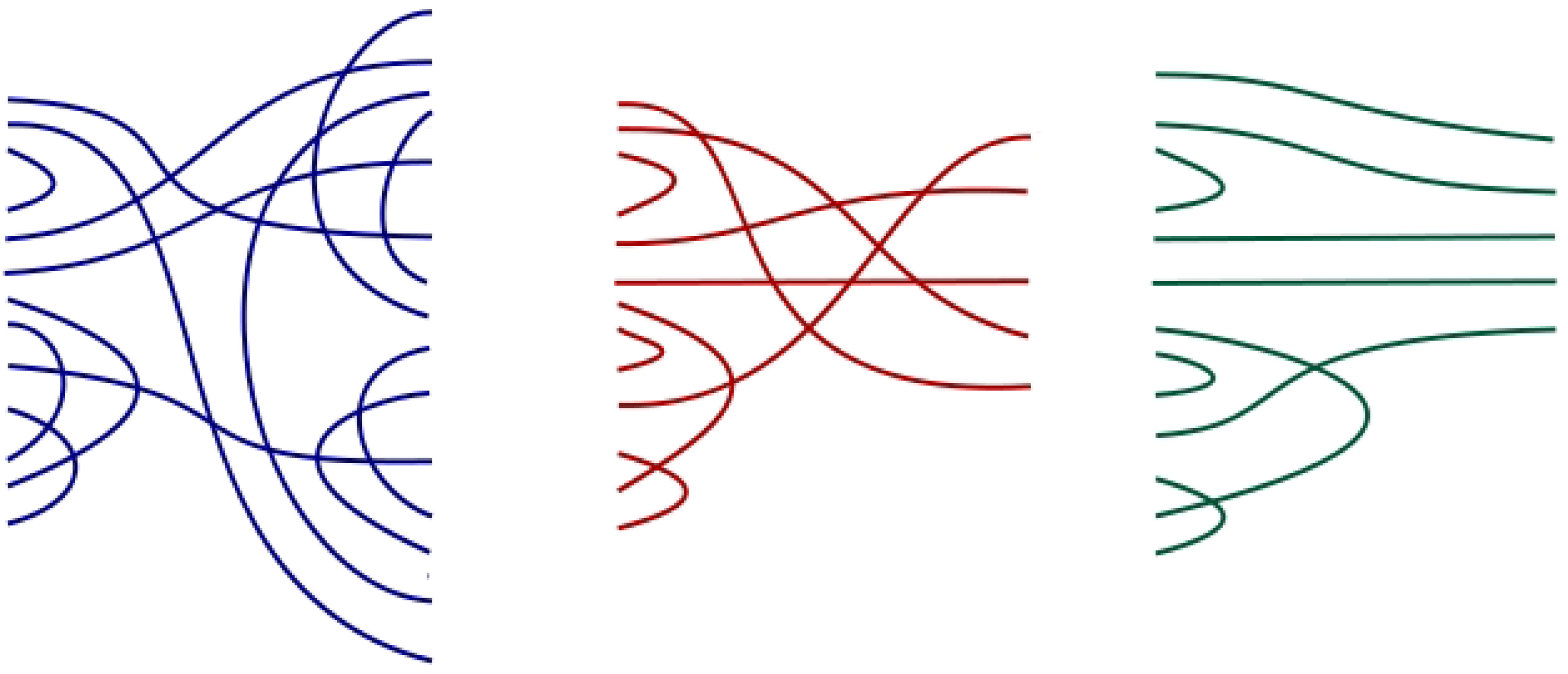
However, sometimes the process of finding appropriate diagrams is an integral non-trivial part of categorification process. For example, in the categorification of classes of orthogonal polynomials the choice of diagrams depends on the inner product, more precisely on the value of the inner product between monomials. In the categorification of the Chebyshev polynomials [23,24] the inner product $(x^n,x^m)=\frac{1}{\frac{n+m}{2}+1}\left(\begin{array}{c}n+m\\ \frac{n+m}{2}\end{array}\right)$ is equal to the $\frac{n+m}{2}$th Catalan number, which is a hint that we can use crossingless matchings on $n+m$ points in our categorification. Similarly, in the case of the Hermite polynomials, the inner product $(x^n,x^m)$ is equal to the double factorial $(n+m-1)!!$, which can be interpreted as the number of all possible ways of connecting $n+m$ points to each other when the crossings are allowed. The details of the construction can be found in papers [23,24], and we will describe the diagrams of basis elements in projective, big standard, and standard (Verma) modules in categorification of the Hermite polynomials, see Figure 19. These diagrams will have a fixed number of right endpoints and an arbitrary number of left endpoints. On the leftmost diagram corresponding to the projective modules, all possible connections between left and right endpoints are allowed, and as we are moving to the right, we introduce additional restrictions. The diagrams in the middle can not contain right returns (arcs connecting one point on the right to another point on the same side), and the diagrams on the very right also can not contain intersections between arcs connecting left to one of the endpoints on the right.

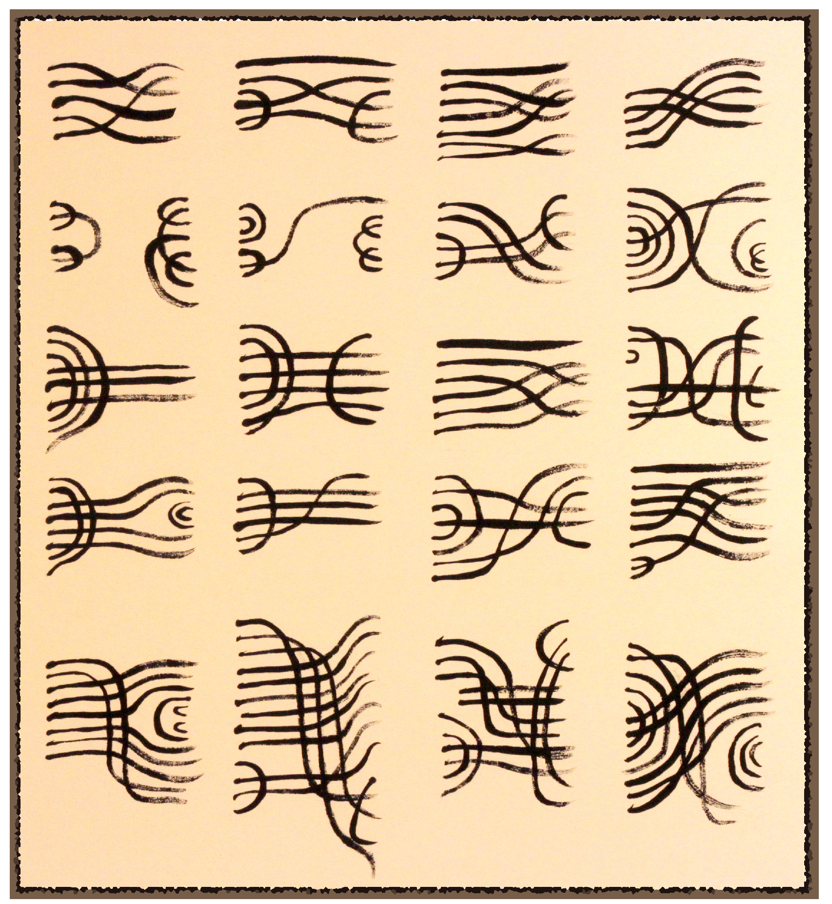
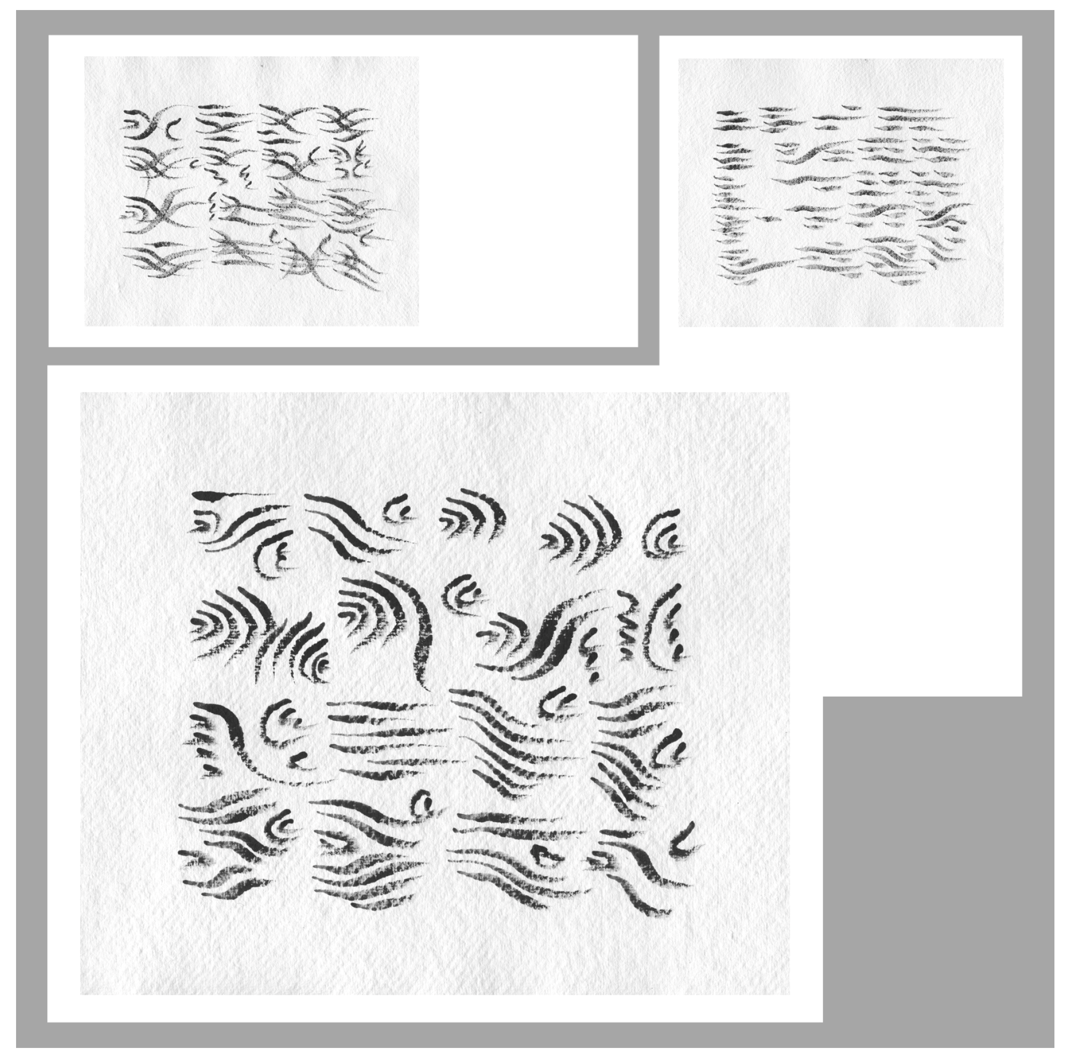
Inspired by different kinds of diagrams used in categorifications of the one-variable polynomial ring with integer coefficients, the Aftermoon studio, Paris, created drawing Tryptique. In the realm of mathematics, they represent elements of three distinct algebras: on the level of Grothendieck rings, projective modules spanned by these diagrams correspond to Chebyshev polynomials, integer powers of x and $(x-1)$, and Hermite polynomials. Taken out of the context, they can be reinterpreted in different ways. Hiroko and Ritsuko Izuhara view them as traditional form of Japanese calligraphy, based on ideas of Dirk Huylebrouck and drawings of R. Sazdanovic. Figure 20 shows their vision of diagrams used in the categorification on Hermite polynomials drawn in ink (sumi) on mulberry paper (washi). Diagrams in Figure 20 and Figure 21 share the mathematical context with ones on Figure 19, with the additional sophistication coming from the medium in which they were realized, and the artists’ take on them. Similar to the way clef and tempo modify the sound of the notes in a staff, the strokes and pressure add expressiveness and sensibility to diagrams. In words of A. Jorn commenting about P. Alechinsky’s work:

“L’image est écrite et l’écriture forme des images... on peut dire qu’il y a une écriture, une graphologie dans toute image de même que dans toute écriture se trouve une image.”

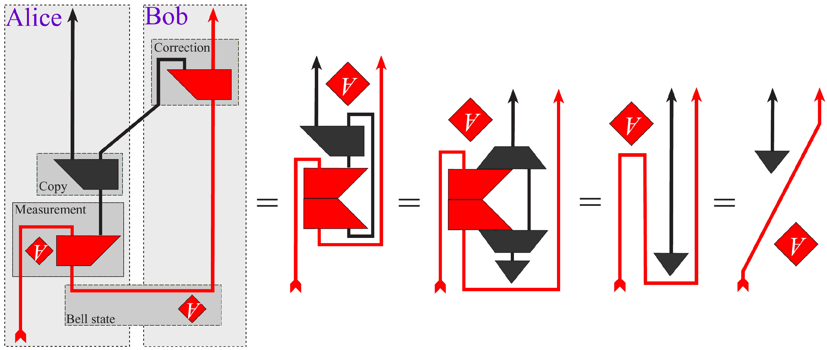
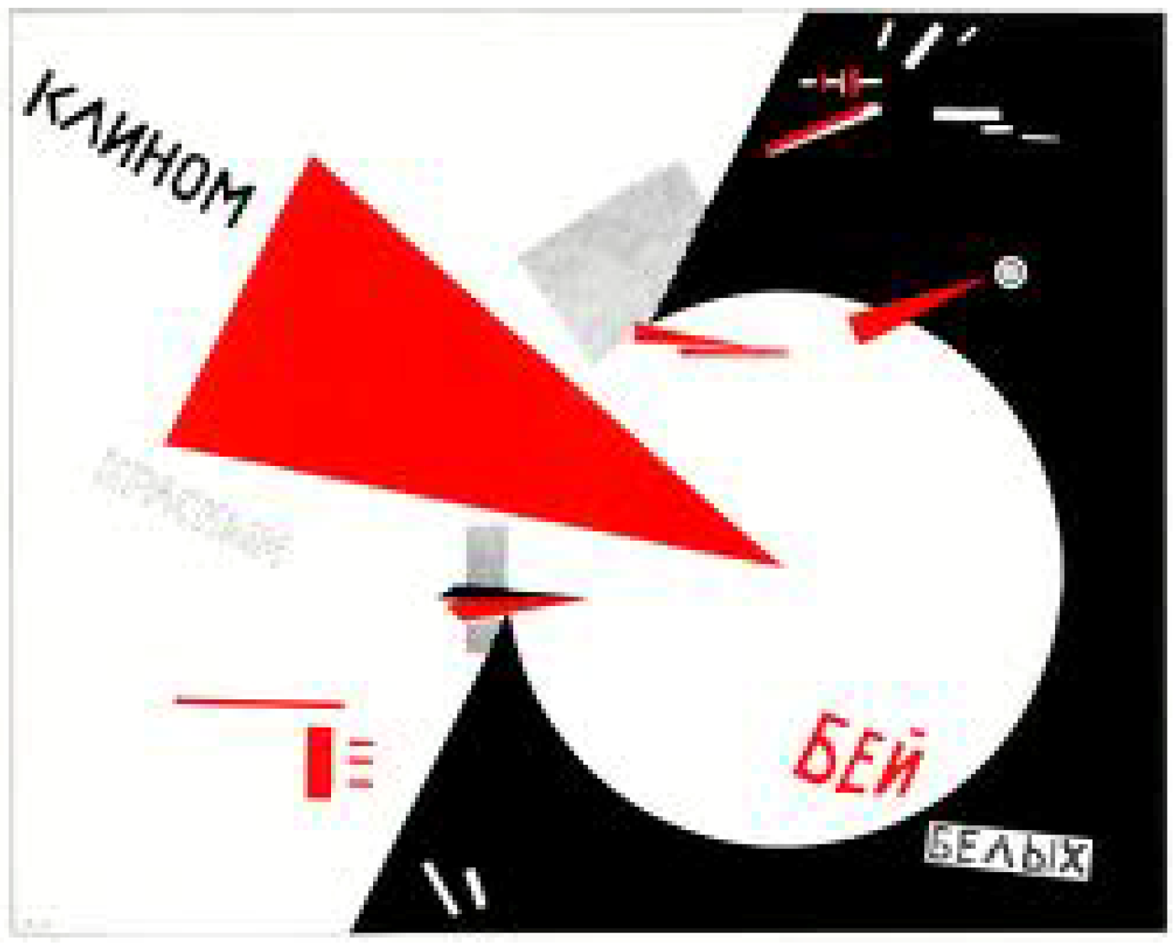
This analogy was taken a step further by S. Abramsky and B. Coecke [25]. They have developed a diagrammatic language for quantum physics, which can be useful in computational linguistic for natural language processing [26]. Their work relies on the well known diagrammatics calculi for category theory and provides “a diagrammatic high-level alternative for the Hilbert space formalism, one which appeals to our intuition” [27,28]. Their graphical calculus simplifies proofs, derivations and computations in quantum theory, and provides a natural framework for describing various phenomena such as quantum entanglement, including quantum teleportation Figure 22. Lastly, notice a very strong visual similarity between the work of Russian constructivist El Lissitzky in his 1919 lithographic poster Beat the Whites with the Red Wedge [29] and a “diagrammatic system for doing quantum mechanics using only pictures of lines, squares, triangles and diamonds” [27,28], when they are deprived of their cultural and scientific connotations, see Figure 22 and Figure 23.

References

- Kirby, R. A calculus for framed links in S3. Invent. Math. 1978, 45, 35–56. [Google Scholar] [CrossRef]
- Johnson, N. Visualizing Seven-Manifolds, short movie presented at the Second Abel Conference: A Mathematical Celebration of John Milnor, Institute for Mathematics and its Applications, Minneapolis, MN, 2012. Animation available online: http://www.nilesjohnson.net/seven-manifolds (accessed on 1 May 2012).
- Khovanov, M. A categorification of the Jones polynomial. Duke Math. J. 2000, 101, 359–426. [Google Scholar] [CrossRef]
- Bray, H.L. Dark matter webpage and MathLab software. Available online: http://www.math.duke.edu/ bray/darkmatter/darkmatter.html (accessed on 1 May 2012).
- Bray, H.L. On Dark matter, spiral galaxies, and the axioms of general relativity. 2010. Available online: http://arxiv.org/abs/1004.4016 (accessed on 1 May 2012).
- Locher, J.L.; Escher, M.C. Escher: The Complete Graphic Work, Thames and Hudson, 1992.
- Knezevic, I.; Sazdanovic, R.; Vukmirovic, S. Visualization of the Lobachevskian Plane. Vis. Mathe. Art Sci. Electron. J. 2002, 4. Available online: http://www.mi.sanu.ac.rs/vismath/sazdanovic/home.htm (accessed on 1 May 2012).
- Knezevic, I.; Sazdanovic, R.; Vukmirovic, S. Basic Drawing in the Hyperbolic Plane, MathSource, Wolfram research 2002. Available online: http://library.wolfram.com/infocenter/MathSource/4260/ (accessed on 1 May 2012).
- Sazdanovic, R.; Sremcevic, M. Tessellations of the euclidean, elliptic and hyperbolic plane. Symmetry Art Sci. 2002, 2, 229–304. [Google Scholar]
- Sazdanovic, R.; Sremcevic, M. Hyperbolic tessellations by tess. Symmetry Art Sci. 2004, 1, 226–229. [Google Scholar]
- Sazdanovic, R.; Sremcevic, M. Tessellations of the euclidean, elliptic and hyperbolic plane, mathsource, wolfram research. 2002. Available online: http://library.wolfram.com/infocenter/MathSource/4540/ (accessed on 1 May 2012).
- Jablan, S.; Sarhangi, R.; Sazdanovic, R. Modularity in medieval persian mosaics: textual, empirical, analytical and theoretical considerations. 2004. Available online: http://www.mi.sanu.ac.rs/vismath/sarhangi/index.html (accessed on 1 May 2012).
- Scharein, R. KnotPlot. Available online: http://knotplot.com/ (accessed on 1 May 2012).
- Sazdanovic, R.; Stipsic, V.; Vujic, M. Tying and untying, movie. 2010. Available online: http://www.youtube.com/watch?v=Bz_A6nhrZMw (accessed on 1 May 2012).
- Jablan, S.; Sazdanovic, R. Discovering symmetry of knots by using program LinKnot. Symmetry Art Sci. 2004, 1, 102–106. [Google Scholar]
- Jablan, S.; Sazdanovic, R. Visualizing symmetry of knots by using program LinKnot. Symmetry Art Sci. 2004, 1, 106–110. [Google Scholar]
- Jablan, S.; Sazdanovic, R. LinKnot: Knot Theory by Computer; World Scientific Publishing Company: Hackensack, NJ, USA, 2007. [Google Scholar]
- Jablan, S.; Sazdanovic, R. LinKnot- Mathematica package. Available online: http://www.mi.sanu.ac.rs/vismath/linknot/index.html (accessed on 1 May 2012).
- Kalantari, B. Polynomial Root-Finding and Polynomiography; World Scientific Publishing Co. Inc.: River Edge, NJ, USA, 2008. [Google Scholar]
- Kalantari, B. Polynomiaography. Available online: http://www.polynomiography.com/java.php (accessed on 1 May 2012).
- Carter, S.J.; Saito, M. Knotted Surfaces and Their Diagrams; American Mathematical Society: Providence, RI, USA, 1991. [Google Scholar]
- Bar-Natan, D. On Khovanov’s categorification of the Jones polynomial. Alg. Geom. Top. 2002, 2, 337–370. [Google Scholar] [CrossRef]
- Khovanov, M.; Sazdanovic, R. Categorifications of the polynomial ring. Available online: http://arxiv.org/pdf/1101.0293v1.pdf (accessed on 1 May 2012).
- Khovanov, M.; Sazdanovic, R. Categorifications of orthogonal polynomials. In preparation.
- Abramsky, S.; Coecke, B. A categorical semantics of quantum protocols. In Proceedings of the 19th Annual IEEE Symposium of Logic in Computer Science, Turku, Finland, July 2004; pp. 415–425. [Google Scholar]
- Coecke, B.; Sadrzadeh, M.; Clark, S. Mathematical foundations for a compositional distributional model of meaning. Linguist. Anal. 2010, 36, 345–384. [Google Scholar]
- Coecke, B. Quantum picturalism. Contemp. Phys. 2010, 51, 59–83. [Google Scholar] [CrossRef]
- Coecke, B. Kindergarten quantum mechanics. 2005. Available online: http://arxiv.org/abs/quant-ph/0510032 (accessed on 1 May 2012).
- Albrecht, W.R. EL - wie Lissitzky. Das Knstlerporträt Liberal 1993, 35, 50–60. [Google Scholar]
Figure 1.
Snapshot from a short movie Visualizing Seven-Manifolds by Niles Johnson.
Figure 2.
Spiral galaxy NGC3310 on the left, simulation on the right.
Figure 3.
M.C. Escher Circle Limit IV (Heaven and Hell), 1960, Woodcut Printed from Two Blocks and Angels and Demons.
Figure 4.
Spherical or elliptic (3,3,3,3,5), Euclidean (3,3,3,3,6) and hyperbolic (3,3,3,3,7) tessellations.
Figure 5.
Escher-like tessellation determined by symbol (6,6,6,6), superimposed with the wire model of the basic tessellation on the right.